Non-Intrusive Load Monitoring: A Review and Outlook

arXiv:1610.01191v1 [cs.OH] 4 Oct 2016

Non-Intrusive Load Monitoring: A Review and Outlook Christoph Klemenjak∗ Peter Goldsborough† October 6, 2016

Abstract With the roll-out of smart meters the importance of effective nonintrusive load monitoring (NILM) techniques has risen rapidly. NILM estimates the power consumption of individual devices given their aggregate consumption. In this way, the combined consumption must only be monitored at a single, central point in the household, providing various advantages such as reduced cost for metering equipment. In this paper3 we discuss the fundamental building-blocks of NILM, first giving a taxonomy of appliance models and device signatures and then explaining common supervised and unsupervised learning methods. Furthermore, we outline a fundamental algorithm that tackles the task of NILM. Subsequently, this paper reviews recent research that has brought novel insight to the field and more effective techniques. Finally, we formulate future challenges in the domain of NILM and smart meters.

1

Introduction

Non-Intrusive Load Monitoring (NILM) techniques extract the power consumption of single appliances out of aggregated power data. Given that a measurement device employing NILM must only installed at a single point, none of the individual appliances have to be equipped with metering devices. In Carinthia, Austria, field trials using such technology are currently being implemented 4 . These smart measurement devices, installed by energy suppliers, pave the way for sophisticated disaggregation algorithms and possibly also recommender-systems. Such a system would be able to detect devices that have a need for maintenance and give appliance-specific feedback to the consumer. ∗ Alpen-Adria-Universit¨ at Klagenfurt, Lakeside Park B10a, 9020 Klagenfurt, [email protected] † Technische Universit¨ at M¨ unchen, Arcisstrasse 21, 80333 M¨ unchen, [email protected] 3 A shorter version of this paper was presented at the SKILL Students Conference 2016, part of the INFORMATIK2016 congress 4 http://gewerbe.kelag.at/content/page strom smartmeter.jsp

1

NILM: A Review and Outlook

Especially older household devices consume a lot more energy than new ones. In [1] measurements of an aged household refrigerator are reported that consumed three times more energy than a new refrigerator. This is a very specific example of a problem that could be solved by load-disaggregation systems. Moreover, research has shown that appliance-specific feedback can save up to 12 % of annual power consumption [2]. Data acquisition units such as smart meters operate at a central point in the household’s power distribution network, generating measurement data of the total power consumption. Currently available commercial smart meters were shown to have a measurement deviation of 10-20 % [3].This shows clearly that actions have to be taken to improve future metering units. [4] states that the recent trend of metering units to make use of more sophisticated energy monitoring ICs, providing more precise measurements, has improved the effectiveness of NILM. This paper is further structured as follows: Before discussing NILM algorithms, the rudimentary concepts and fundamental vocabulary of the field will be introduced. To investigate appliances, we must first classify them according to their particular features and behaviour. This step is examined in Section 2. Once measurement data is available, it must be analysed to extract relevant appliance signatures, allowing tracking of said appliances. We examine this topic in Section 3. Naturally, a NILM system requires to be aware about the circuits it is monitoring and thus to detect them. For this, a wide range of learning approaches are applied, which we discuss in Section 4. After touching upon these introductory concepts, we describe a fundamental NILM algorithm published by Hart [5]. Since the publication of this algorithm in 1992, the field of load-disaggregation has seen a tremendous amount of further research and novel approaches. We present a selection of these ideas in Section 8. Lastly, in Section 9, we discuss future challenges faced by the NILM community.

2

Appliance types

Appliances differ in the number of operational states and their power consumption behaviour. For the purpose of further discussion and analysis, we therefore present three abstract models that are commonly used in research to represent and characterise appliances. In detail, we will examine models for on/off appliances, multi-state appliances and infinite-state appliances.

2.1

On/Off appliances

The first type of device is the so-called on/off appliance. This class includes common household appliances such as a toaster or a light bulb. Such appliances consume only one specific amount of power when active. For the large part, on/off appliances are purely resistive. Appliances with a small reactive part are assumed to be linear. A well-known fact is that electric power is additive. This fact is exploited when describing a set of on/off appliances. The total power consumed at time-instant t is the sum of all power signals Pi (t). To modulate

NILM: A Review and Outlook

the power signal a switch process ai (t) ∈ {0, 1} is introduced. The product of the switch processes and the power signals models the power consumption of a given appliance. The total power Ptotal (t) can therefore be estimated by: Ptotal (t) =

N X

ai (t)Pi (t) + e(t)

(1)

i=1

The additive term e(t) describes the deviation between the actual sum of the modulated power signals and the measured total power. To estimate the state of the appliances, the deviation e(t) has to be minimised. In general, the problem with this is that the complete set of power signals P1 (t) . . . PN (t) is not known. A second issue is that from a high measurement uncertainty in estimating the total power Ptotal (t), a bad interpretation of the switching process may follow. Many appliances may be estimated to be turning on and off at the same time. As a solution the Switch Continuity Principle was introduced in [5]. It states that in a small time interval the number of appliances changing their state is also small. Consequently, we assume that in a small enough time window the number of state transitions is zero. The sampling frequency of the acquisition unit has thus to be high enough to detect such time windows. Between two such intervals, in which the total power consumption is steady, appliances which change their state can be identified.

2.2

Multi-state appliances

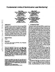
The second type of appliances are multi-state appliances, which have more than one state of operation. Each of these states has a specific power consumption. A common way to represent this class of devices is the finite state machine (FSM) model. The graphic rendition of such a FSM consists of several circles, each corresponding to a specific state of operation with a well-defined power consumption. At the transition from one state to the other, visualised by an edge, the power draw increases or decreases by the difference in consumption between the two states of operation. As an example, let there be a finite state machine model with two states of operation, as illustrated in Figure 1. State A represents a power consumption of 500 W and state B a consumption level of 750 W. At the transition from state A to state B the power consumption of the appliance rises with an amount of 250 W. In contrast to that the power consumption decreases by 250 W from state B to state A. This is analogous to Kirchhoffˆ as law, as the sum of the power changes is zero.

2.3

Infinite-state appliances

Lastly, there exist also appliances whose observable set of states is not finite. For example, the power consumption of light-dimmers changes continuously with no consistent step change. Such infinite-state appliances represent a challenge to model and identify. Figure 2 shows the power consumption of such a continuously-varying power consumption. While on/off appliances as well as

NILM: A Review and Outlook

−750W B +750W −250W

+250W

OF F +500W A −500W

Fig. 1: Finite state machine for an electric heater multi-state appliances change their power consumption in one clear and observable step, infinite-state appliance’s power draw shows a smooth pattern. One subclass of infinite-state appliances are those continuously consuming energy, even when set in standby. Examples of such devices include fire detectors or TVs. Power

single

multi

infinite

Time Fig. 2: Power consumption of different appliance types

3

Appliance signatures

Appliance signatures describe characteristics specific to certain devices, which can thus be used to identify and classify them. The importance of such signa-

NILM: A Review and Outlook

tures was already pointed out in [6], where a taxonomy of voltage-current signatures was introduced to classify appliances. In general, appliance signatures can be seen as measurable parameters, which provide device-specific information extracted from physical quantities. Another taxonomy was introduced in [5], where two classes of non-intrusive appliance signatures are described: steadystate signatures and transient-state signatures.

3.1

Steady-state signatures

Steady-state signatures comprise features extracted from appliances when they are not currently transitioning between two states but are operating at a steady level of power consumption. More specifically, a steady-state signature is the result of analysing the difference in certain characteristics between two steady states of operation. Such a characteristic may be, but is not limited to, the change in power consumption as was depicted in Figure 1. In general such features can be categorised into the following groups: • Power Change: Real and reactive power are the physical quantities of greatest interest, since they provide very characteristic information about appliances. To detect such features, the power consumption is estimated and plotted as shown in Figure 3. One major difficulty associated with this is the fact that certain power signatures may overlap. This overlap results in a bad detection probability especially for appliances with low power consumption. Implementations such as [7] implement rely on these signatures. • V-I Features: The problem with overlaps can be solved by adding additional information about the appliances. By analysing the V-I characteristics, for instance the root-mean-squared (RMS) values of voltage and current, appliances with a similar power consumption may be further described and distinguished. • V-I Trajectory: Another method, using current and voltage signals, is to classify devices by extracting features out of the V-I trajectory. The shape of this trajectory shows useful characteristic features such as asymmetry, looping direction, and enclosed area. A recent application of analysing theses features can be found in [8]. • Harmonics: In [5], Hart states that analysing the harmonics of a device’s current waveform by means of a Fourier Analysis can provide additional information about an appliance’s characteristics. In particular, it was found that some non-linear appliances such as motors or light-dimmers produce current waveforms containing a specific set of harmonics, which can further aid in classification. Extraction of such steady-state signatures does not necessarily demand for high-end metering hardware. RMS values of current and voltage as well as frequent power readings provide a good basis to extract steady-state signatures.

NILM: A Review and Outlook

Reactive Power in VAr

1250 1000 750 500 250

400

800

1600 2000 2400 2800 3200 Active Power in W

Fig. 3: Distribution of appliances in a traditional P-Q plane Already low-cost hardware such as introduced in [4] can be used to identify steady-state signatures.

3.2

Transient-state signatures

Situations exist where two different appliances may have very similar power consumption profiles, reducing chances of correct identification of either device. In such cases, examining the transients, i.e. the consumption behaviour of an appliance when transitioning between two steady states of operation, can provide vital information. The transient signature of an appliance is strongly influenced by the physical task it performs [9]. For instance, the turn-on current of a computer system differs massively from a lighting system due to charging capacitors. The shape, size, and duration of such a transient can thus aid in distinguishing between two appliances when their steady-state signatures alone do not provide a sufficient basis for identification. At the same time, as noted in [5], it must be considered that such momentary transition events are less easily detectable than steady-state operation and may require a higher sampling frequency. Another approach takes emitted voltage noise into account. Each appliance in state operation transmits noise back to the power line. This noise can be measured and categorised into on/off transient noise, steady-state line voltage noise and steady-state continuous noise [10].

3.3

Ambient Appliance Features

Both steady-state and transient characteristics are extracted from what are arguably the most obvious sources: the power, voltage or current draw of an

NILM: A Review and Outlook

appliance. However, in recent research, appliance-specific patterns have also been extracted from environmental, ambient or behavioural sources. Such techniques exploit the external impact of appliances, such as their heat-dissipation or light-emission. For this purpose, [11] advocates the collection of data from environmental sensors. An implementation of this idea was proposed in [12], where the deployment of electromagnetic field detectors (EMF) to combine information about energy wastage and power-consumption profiles was examined. In the same spirit, [13] discusses the fact that home appliances emit sound waves (noise). A system is suggested that correlates information about energy consumption with sound recordings of the respective appliance. In contrast to information provided by sensors about appliances directly, there exists also the paradigm of Context-Aware Power Management (CAPM) [14]. CAPM techniques typically examine signatures not necessarily extracted from appliances themselves, but from their environment, users or usage behaviour. For instance, [15] explores behavioural patterns including duration of use and time of day. In [15] and [2] it is stated that such contextual information may also include location or even weather patterns. Furthermore, [16] studies appliance-user interaction to facilitate load-disaggregation. The behaviour and presence of human beings is traced by a set of motion sensors in the building and combined with other NILM techniques. To gather such ambient data, a wireless sensor network was proposed by [14].

3.4

Optimal Sampling Frequency for Signature Detection

The number and kinds of steady-state and transient appliance features recognisable from an aggregated consumption sample is strongly connected to the frequency of measurement in the earliest stages of disaggregation. As noted in [17], a wide range of utilised sampling frequencies is reported in past literature. Many of the steady-state appliance features described above, such as current harmonics or V-I trajectories and especially transient features are more realistically attainable at higher sampling frequencies. With high frequencies we usually mean several kHz, although select approaches have even employed MHz readings [18]. High-frequency sampling rates not only allow more finegrained and detailed analysis of device-signatures, but are also more flexible. The obvious benefit of having more samples available than too few, is that when high-resolution data is not required or too bulky to store, it can always be down-sampled to lower frequencies. On the flip side, metering hardware for high sampling rates is practically non-existent in households today, making NILM techniques requiring sampling rates in the region of 1 Hz more practical and immediately applicable. 1 Hz readings as used by Hart’s algorithm [5] allow for reasonably effective examination of active and reactive power measurement. More recently, attempts have been made to better adjust NILM algorithms to the low-frequency sampling of conventional smart meters. For example, [19] makes attempts to perform load disaggregation using discriminative sparse coding techniques on power samples provided only on an hourly basis.

NILM: A Review and Outlook

4

Learning Approaches

Learning approaches for NILM can fundamentally be divided into supervised and unsupervised techniques. The distinction between a supervised and an unsupervised algorithm is whether or not ground-truth data about individual appliance features is available to train the algorithm. If such device-specific information is present, meaning that the algorithm knows a priori about the appliances it is monitoring, the learning approach is limited to disaggregation only. On the other hand, an unsupervised algorithm need not only perform loaddisaggregation, but additionally detect which appliances exist in the circuit it is monitoring.

4.1

Supervised Learning Approaches

Supervised approaches feed the system with existing device-specific information, such as its power consumption profile. This data may either already exist, such as in the case of the REDD dataset [17], or is the result of an initial training phase, in which a database of appliances and their signatures is collected [20]. The actual load-disaggregation is commonly performed by one of two techniques: Optimisation or pattern recognition. We will elaborate on either approach in the following paragraphs. • Optimisation: A straightforward method to solve the load disaggregation task is to model it as optimisation problem. Obtaining the solution for such problems is well-researched and builds on a simple concept. The extracted appliance features are compared to an existing database consisting of appliance features. When the deviation between the database’s entry and the extracted feature can be minimised, the best match is obtained [20]. For a small number of appliances, this approach may very well be feasible. However, as discussed in [21] , the performance of this method deteriorates with an increasing number of loads, while the complexity increases. Another weak point of this approach is that it may have significant difficulties in distinguishing between loads with overlapping signatures. • Pattern Recognition: This approach detects appliances by means of clustering and mapping state-changes to a feature space [10]. An example of such clustering is given in Figure 3. As outlined by Hart in [5], the identified appliance features in the PQ plane are divided into clusters. Given this initial separation, the clusters are compared to those already known to the supervised system. In further detail, [10] identifies two main approaches: Bayesian classifiers and heuristic methods. For the former, it is assumed that two operating states of an appliance are independent of each other. While research has shown promising results for the Bayesian approach, the independence of states is clearly an ideal but not practical model. For example, the power state of a computer monitor usually depends directly on the power state of the connected computer.

NILM: A Review and Outlook

4.2

Unsupervised Learning Approaches

Supervised learning approaches require an initial training phase and input of external, labeled data. Practically speaking, for the average household, such data does not exist. Therefore, unsupervised learning approaches, which are able to operate without a priori information, are a promising alternative. Unsupervised disaggregation techniques are required not only to perform load-disaggregation, but must further train themselves online. This means that appliances need to be identified and extracted from the aggregate power signal and their models added to the database of existing devices. The quality of the load-disaggregation is thus additionally dependent on the ability of the system to correctly identify existing devices. Methods of probabilistic analysis such as Hidden Markov Models (HMMs) and extensions thereof are especially suited to this task [20]. An HMM is a probabilistic graphical model that differs from standard Markov models in that the states are not directly observable, but can only be estimated probabilistically given certain observations. For NILM purposes, an appliance can be described as an HMM with n hidden states S = {s1 , ..., sn } representing the appliance’s states of operation. Also, we define an observation or emission matrix describing the probability for the appliance to be in a certain state s at time slice t given the observation (emission) of an aggregate power consumption signal. Lastly, there exists a transition matrix T = (ai,j ) ∈ Rn×n where ai,j represents the likelihood for a transition of the appliance from state si to state sj between two time slices Pt and t + 1. More specifically, ai,j = P (xt+1 = sj |xt = si ) with ai,j > 0 and nj=0 ai,j = 1. Factorial Hidden Markov Models (FHMM) are an extension of the basic HMM. An FHMM models not only a single but many independent hidden state chains in parallel, with the emission (the aggregate power consumption) being thus a function of all states combined. In [21] it is stated that this can help reduce the number of parameters maintained by the system.

5

Hart’s NILM algorithm

The algorithm introduced by Hart in [5] is considered fundamental in the NILM community and is the basis of many of today’s load-disaggregation techniques. For this reason, we will outline its basic operation briefly. The general concept of Hart’s algorithm is to meter a household’s aggregate power consumption, identify appliances and then track their behaviour. The algorithm executes the following tasks: 1. Measure Power and Voltage: Measurements of the aggregate power and RMS voltage signal are recorded at a sampling frequency of 1 Hz. 2. Calculate Normalised Power: The estimated power signals are normalised (smoothed) depending on the power line voltage. This allows for immediate comparison of power levels.

NILM: A Review and Outlook

3. Edge Detection: An edge-detection algorithm is applied to the normalized power signals. This algorithm extracts steps in power consumption and labels the time instants. 4. Cluster Analysis: The output of the edge detection algorithm is used to create points in the PQ-plane. Points nearby are clustered. 5. Build Appliance Models: From the clusters obtained finite state machine (FSM) models are created. The simplest state machine is an on/off appliance consisting of two symmetrical events at the PQ-plane. 6. Track Behaviour: The estimated appliance models are tracked. Whenever a modelled appliance performs a state transition, the algorithm recognises this behaviour. 7. Tabulate Statistics: Statistics and characteristics of the models obtained so far are calculated and tabulated. These statistics may also be used to predict the future behaviour of the monitored state machines. 8. Appliance Naming: In the final step, the algorithm attempts to assign each observed FSM to an actual appliance in the system. For this, Hart recommends Bayesian, maximum-likelihood-multiple-hypothesis or other methods from detection theory.

6

Evaluation Metrics for NILM Algorithms

To evaluate the performance and quality of a load-disaggregation algorithm, numerous accuracy metrics are reported in NILM literature. We have identified no common agreement in the community on which metrics are superior or more suitable to certain approaches. This in particular can bar the way to a quantitative comparison of different NILM techniques. We will nevertheless outline the general categories of evaluation metrics and briefly touch upon specific examples. We also wish to note and laud up-front the work of Batra, Kelly et al. in publishing NILMTK, an open-source toolkit for evaluating NILM algorithms that implements many of the metrics discussed below [22] 5 .

6.1

Event-Based Metrics

Event-based metrics focus on evaluating the detection of state-changes in the operation of appliances. More specifically, it is analysed how well an algorithm can identify an appliance switching on or off [20]. Event-based metrics make use of the terms True Positive (TP), True Negative (TN), False Positive (FP) and False Negative (FN). TP refers to the number of times a device is correctly identified as on, while TN is the count of correctly captured off events. Conversely, a FP event stands for the case when an active state was reported, when 5 http://nilmtk.github.io

NILM: A Review and Outlook

the device was in fact not consuming power. FN is defined analogously. Given these quantities, the following evaluation metrics can be calculated: • Precision: The ratio of samples an appliance was correctly detected as active: TP P recision = ∈ [0, 1] (2) TP + FP • Recall: The ratio of samples the algorithm captured an actual turn-on event: TP Recall = ∈ [0, 1] (3) TP + FN • Accuracy: The ratio of samples the algorithm correctly identified the actual state of an appliance: Accuracy =

6.2

TP + TN ∈ [0, 1] TP + TN + FP + FN

(4)

Non-Event-Based Metrics

Non-event-based metrics analyse how well a load-disaggregation algorithm is able to compute and assign the power-consumption of individual appliances [22]. One drawback of such metrics is that may produce favourable quantitative results for appliances that are inactive for long spans of time, shadowing the ability of an algorithm to identify a device’s power draw in one of its active operating states. Given that most household appliances such as televisions or microwaves are inactive for the majority of the day, an algorithm may score very highly on such a non-event-based metric simply by assigning zero power consumption to all appliances. As stated in [17], this class of metrics is nevertheless applicable to a wider range of algorithms, as it does not mandate the extraction of edges from the aggregate power signal. One such evaluation criterion, as reported in [22], is the root mean square error (RMSE). More specifically, the RMSE between the identified power draw and the actual power draw of an appliance is given by the equation: s P (n) (n) − yˆt )2 t (yt RM SE = (5) T (n)

Where T denotes the number of samples recorded, yt the assigned power draw of the n-th appliance at time instant t, and yˆ the actual power draw of that appliance at that time instant. Another variation of this metric, as employed by [21], is to normalise the RMSE over the range of all recorded samples, yielding the normalised RMSE (NRMSE): N RM SE =

RM SE (n) max(yt )

(n)

− max(yt )

(6)

NILM: A Review and Outlook

6.3

Overall Metrics

Lastly, another class of metrics exists which evaluates the overall performance of a load-disaggregation algorithm. In the simplest scenario, one would rate the quality of a NILM technique by calculating the percentage of the total power assigned to a specific appliance for the entire duration of the experiment, relative to the aggregate consumption of all appliances [17]. One would then inspect the difference between this value and the ground truth quantity, calculated P (n) identically. Let Yt = n yt denote the total aggregate power consumption estimated at time t, and Yˆt the ground-truth equivalent. The average deviation in the ratio between assigned and actual power consumption may be calculated as: P P (n) (n) (ˆ y ) 1 X t (yt ) − Pt t ) (7) ( P ˆ N n t (Yt ) t (Yt )

7

Datasets for NILM Research

There exist a number of publicly available datasets to test and train the various aforementioned learning approaches. We have picked two such datasets for the purpose of further discussion and analysis of their characteristics.

7.1

The Reference Energy Disaggregation Data Set

One of the most detailed and widely used datasets is the Reference Energy Disaggregation Data Set (REDD) [17]. It was released to the public for purposes of load-disaggregation research by MIT in 2011. REDD is composed of aggregated as well as sub-metered, device-specific power-consumption data gathered from 10 homes monitored over a period of two weeks. In total, it contains a combined 119 days of measurements spread over 1 terabyte of data. High as well as low frequency samples were extracted from three separate sources: 1. Mains electricity, sampled at 15 kHz. 2. Labeled circuits, recorded at 0.5 Hz. 3. Plug-level monitors, gathered at 1 Hz. While REDD finds its use in sources such as [21] and [23], it is mentioned in [20] that the total aggregate of individual appliances’ power consumptions at certain time points differs from the mains measurement reported in the dataset. As also noted in [20], this inconsistency indicates the existence of additional, unmeasured devices.

NILM: A Review and Outlook

7.2

GREEND

Another publicly available dataset is GREEND, released by Monacchi et al. in 2014 [24]. GREEND consists of active power measurements of nine houses for a continuous duration of one year, collected in the region of Carinthia, Austria and Friuli-Venezia, Italy. Each house contains an average of nine appliances, totaling 79 different power-consumption sources. It claims to be the first power-consumption dataset for Austria and Italy measured at a 1 Hz samplingfrequency. The long period of measurement in particular makes GREEND very attractive for NILM research, allowing investigation and modeling of seasonal consumption behaviour. Other datasets such as REDD, lasting approximately two weeks [17], or BLUED [25], spanning 8 days, comprise much less data, in comparison.

8

Recent approaches

A more recent approach suggests a rethinking of NILM itself and introduces a new way of implementing the algorithm. The authors of [26] introduce a new modelling of NILM in a application-centric way. The approach demands for realtime processing right after metering, which is termed online NILM. Basically it is suggested to divide NILM into three steps: device detection, modelling, and device-tracking. The novelty of this approach is that device detection and modelling are usually said to be offline tasks as part of algorithm-training. For the method proposed, device recognition and monitoring is implemented online and in real-time. Smart meters would thus transmit the measurement data immediately to the cloud or server. For example, the online service could be hosted by the power utility itself, improving its immediate ability to forecast future power consumption. The crux of this idea lies in computation. Such a system would have to perform NILM across hundreds of households in real-time. We identify this in particular as a challenge. The most common learning algorithms used for load-disaggregation today rely on optimisation or Factorial Hidden Markov Models (FHMM). In [27], Kelly et al. very recently employed a novel learning approach based on artificial neural networks (ANN). For this, the authors implemented three separate ANN architectures. The first is a recurrent neural network, which learns appliance features on a training dataset to then estimate the appliance consumption level given an aggregate sample. The second architecture utilises a denoising autoencoder (dAE), often used for signal reconstruction and denoising, such as for removing grain from an old image or reverberation from an audio track. For the dAE, the learning task is to extract a device’s load from an aggregate sample, by viewing the consumption of other appliances as the signal’s unwanted noise component. Lastly, a standard neural network was used to regress start and end time as well as power consumption for each activation of a device. We note that little research has been done on the application of these modern machine learning techniques to NILM. Yet, [27] shows that neural networks beat conven-

NILM: A Review and Outlook

tional load-disaggregation algorithms in almost every metric, inviting further investigation into these promising new learning approaches.

9

Conclusion

In this paper we discussed the concept of NILM, appliance models, appliance signatures and learning methods as well as recent improvements and trends in the field of load-disaggregation. We are certain further research is necessary. One fundamental question posed is where and on what platforms data processing and NILM algorithms are performed. The first and simplest option is the measurement device itself, meaning the smart meter or metering units installed in the household. This would require sophisticated hardware that is capable of performing NILM in real-time. In general, such hardware is more expensive and energy-consuming than conventional measurement devices. Therefore another approach is to perform data processing on a device in the home network. Single-board computing devices such the Raspberry Pi6 or BeagleBoard7 could be well suited to such a task. With the surge of cloud-computing services in recent years, the employment of such an online service becomes a possibility as well. However, along with data-transmission across networks, away from the home and into the cloud, security concerns will and must be raised. We estimate that the majority of the population would feel unease in sending their private household data to external servers. In conclusion, we would like to re-emphasise our belief in the very certain potential of load-disaggregation techniques to improve the consumption patterns of individuals and reduce energy wastage in the grid. At the same time, we acknowledge that non-intrusive load-monitoring is still a very open and ongoing field of research and that no current approach is perfect. We express our hope that this will change in the near future.

References [1] D. Benyoucef, P. Klein, and T. Bier, “Smart meter with non-intrusive load monitoring for use in smart homes,” in IEEE International Energy Conference, 2010, pp. 96–101. [2] K. C. Armel, A. Gupta, G. Shrimali, and A. Albert, “Is disaggregation the holy grail of energy efficiency? The case of electricity,” Energy Policy, vol. 52, no. 0, pp. 213 – 234, 2013. [3] M. Zeifman and K. Roth, “Nonintrusive appliance load monitoring: Review and outlook,” IEEE Transactions on Consumer Electronics, pp. 76–84, 2011. 6 https://www.raspberrypi.org 7 https://beagleboard.org

NILM: A Review and Outlook

[4] C. Klemenjak, D. Egarter, and W. Elmenreich, “Yomo: the arduino-based smart metering board,” Computer Science-Research and Development, pp. 1–7, 2015. [5] G. W. Hart, “Nonintrusive appliance load monitoring,” Proceedings of the IEEE, vol. 80, no. 12, pp. 1870–1891, 1992. [6] K. Ting, M. Lucente, G. S. Fung, W. Lee, and S. Hui, “A taxonomy of load signatures for single-phase electric appliances,” in IEEE PESC (Power Electronics Specialist Conference), 2005, pp. 12–18. [7] S.-J. Huang, C.-T. Hsieh, L.-C. Kuo, C.-W. Lin, C.-W. Chang, and S.A. Fang, “Classification of home appliance electricity consumption using power signature and harmonic features,” in Power Electronics and Drive Systems (PEDS), 2011 IEEE Ninth International Conference on. IEEE, 2011, pp. 596–599. [8] T. Hassan, J. Fahad, and N. Arshad, “An empirical investigation of v-i trajectory based load signatures for non-intrusive load monitoring,” IEEE Transactions on Smart Grid, vol. 5, no. 2, pp. 4–31, Mar 2014. [9] C. Laughman, K. Lee, R. Cox, S. Shaw, S. Leeb, L. Norford, and P. Armstrong, “Power signature analysis,” IEEE power and energy magazine, pp. 56–63, 2003. [10] A. Zoha, A. Gluhak, M. A. Imran, and S. Rajasegarar, “Non-intrusive load monitoring approaches for disaggregated energy sensing: A survey,” Sensors, vol. 12, no. 12, pp. 16 838–16 866, 2012. [11] M. Berg´es, L. Soibelman, and H. S. Matthews, “Leveraging data from environmental sensors to enhance electrical load disaggregation algorithms,” in Proceedings of the 13th International Conference on Computing in Civil and Building Engineering, Nottingham, UK, vol. 30, 2010. [12] M. Berg´es and A. Rowe, “Appliance classification and energy management using multi-modal sensing,” in Proceedings of the Third ACM Workshop on Embedded Sensing Systems for Energy-Efficiency in Buildings. ACM, 2011, pp. 51–52. [13] M. A. Guvensan, Z. C. Taysi, and T. Melodia, “Energy monitoring in residential spaces with audio sensor nodes: Tinyears,” Ad Hoc Networks, vol. 11, no. 5, pp. 1539–1555, 2013. [14] A. K. Dey, G. D. Abowd, and D. Salber, “A conceptual framework and a toolkit for supporting the rapid prototyping of context-aware applications,” Human-computer interaction, vol. 16, no. 2, pp. 97–166, 2001. [15] J. Z. Kolter and T. Jaakkola, “Approximate inference in additive factorial hmms with application to energy disaggregation,” in

NILM: A Review and Outlook

Proceedings of the Fifteenth International Conference on Artificial Intelligence and Statistics (AISTATS-12), N. D. Lawrence and M. A. Girolami, Eds., vol. 22, 2012, pp. 1472–1482. [Online]. Available: http://jmlr.csail.mit.edu/proceedings/papers/v22/zico12/zico12.pdf [16] N. B. Priyantha, A. Kansal, M. Goraczko, and F. Zhao, “Tiny web services: design and implementation of interoperable and evolvable sensor networks,” in Proceedings of the 6th ACM conference on Embedded network sensor systems. ACM, 2008, pp. 253–266. [17] J. Z. Kolter and M. J. Johnson, “Redd: A public data set for energy disaggregation research,” in Workshop on Data Mining Applications in Sustainability (SIGKDD), San Diego, CA, vol. 25. Citeseer, 2011, pp. 59–62. [18] S. Gupta, M. S. Reynolds, and S. N. Patel, “Electrisense: Single-point sensing using emi for electrical event detection and classification in the home,” in Proceedings of the 12th ACM International Conference on Ubiquitous Computing, ser. UbiComp ’10. New York, NY, USA: ACM, 2010, pp. 139–148. [Online]. Available: http://doi.acm.org/10.1145/1864349.1864375 [19] J. Z. Kolter, S. Batra, and A. Y. Ng, “Energy disaggregation via discriminative sparse coding,” in Advances in Neural Information Processing Systems 23, J. Lafferty, C. Williams, J. Shawe-taylor, R. Zemel, and A. Culotta, Eds., 2010, pp. 1153–1161. [Online]. Available: http://books.nips.cc/papers/files/nips23/NIPS2010 1272.pdf [20] M. Aiad and P. Lee, “Unsupervised approach for load disaggregation with devices interactions,” Energy and Buildings, vol. 116, pp. 96–103, 2016. [21] D. Egarter, V. Bhuvana, and W. Elmenreich, “Paldi: Online load disaggregation via particle filtering,” IEEE Transactions on Instrumentation and Measurement, vol. 64, no. 2, pp. 467–477, 2015. [22] N. Batra, J. Kelly, O. Parson, H. Dutta, W. Knottenbelt, A. Rogers, A. Singh, and M. Srivastava, “NILMTK: An Open Source Toolkit for Nonintrusive Load Monitoring,” ArXiv e-prints, Apr. 2014. [23] O. Parson, “Unsupervised training methods for non-intrusive appliance load monitoring from smart meter data,” April 2014. [Online]. Available: http://eprints.soton.ac.uk/364263/ [24] A. Monacchi, D. Egarter, W. Elmenreich, S. D’Alessandro, and A. M. Tonello, “GREEND: an energy consumption dataset of households in italy and austria,” CoRR, vol. abs/1405.3100, 2014. [Online]. Available: http://arxiv.org/abs/1405.3100 [25] F. Englert, T. Schmitt, S. K¨oßler, A. Reinhardt, and R. Steinmetz, “How to auto-configure your smart home?: High-resolution power measurements to the rescue,” in Proceedings of the fourth international conference on Future energy systems. ACM, 2013, pp. 215–224.

NILM: A Review and Outlook

[26] S. Barker, S. Kalra, D. Irwin, and P. Shenoy, “Nilm redux: The case for emphasizing applications over accuracy,” in NILM-2014 Workshop, 2014. [27] J. Kelly and W. J. Knottenbelt, “Neural NILM: deep neural networks applied to energy disaggregation,” CoRR, vol. abs/1507.06594, 2015. [Online]. Available: http://arxiv.org/abs/1507.06594