identification; Sparse subspace learning; Hierarchical collocation ...... Simulation were scripted using Python and a Matlab generic interface was used to.
Non-intrusive sparse subspace learning for parametrized problems Domenico Borzacchiello Jos´e V. Aguado Francisco Chinesta Abstract We discuss the use of hierarchical collocation to approximate the numerical solution of parametric models. With respect to traditional projection-based reduced order modeling, the use of a collocation enables non-intrusive approach based on sparse adaptive sampling of the parametric space. This allows to recover the lowdimensional structure of the parametric solution subspace while also learning the functional dependency from the parameters in explicit form. A sparse low-rank approximate tensor representation of the parametric solution can be built through an incremental strategy that only needs to have access to the output of a deterministic solver. Non-intrusiveness makes this approach straightforwardly applicable to challenging problems characterized by nonlinearity or non affine weak forms. As we show in the various examples presented in the paper, the method can be interfaced with no particular effort to existing third party simulation software making the proposed approach particularly appealing and adapted to practical engineering problems of industrial interest.
Reduced order modeling; Non-intrusiveness; Low rank approximations; Sparse identification; Sparse subspace learning; Hierarchical collocation
1 1.1
Introduction Motivation
Models are often defined in terms of one or several parameters regardless of the nature of the phenomenon they describe. Parameters allow to adaptively adjust a general model to a wide range of different scenarios governed by the same physical laws. In continuum mechanics, for instance, models are expressed mathematically as partial differential equations (PDE) representing the balance or the conservation laws governing the evolution of the fundamental variables that describe the state of a system. Numerical methods for the solution of such differential models have reached in many cases a remarkable degree of maturity, enabling the development of a variety of simulation software. This technological advancement has resulted in a massive usage of the simulation tools at the industrial scale, mainly as a means of solving practical problems such as design, optimization or inverse identification [1]. In this context, the user is usually interested in assessing the adequacy of a particular configuration with regard to a given 1
design or performance criterion. This means in practice that the user decides, based on simulation results, whether a particular design fulfills or not the product specifications, or, in an optimization context, whether the process performance is improved or worsened by a specific setup. The decision-making process based on simulation commonly referred to as simulation-based engineering [2, 3]. In spite of the simplicity of this concept, simulation-based engineering may be somehow limited by the need of evaluating multiple configurations before converging to a satisfactory result, that is, a design that fulfills the product specifications or a setup that optimizes the process performance. This practice, in which simulations have to be carried out for several changing configurations is the foundation of multiquery simulation. Each query (i.e. configuration evaluation) requires allocating some time to prepare a new simulation, execute it and analyze the results. Delays due to communication and information exchange in collaborative work projects should also be taken into account. This may render the design, or optimization, process very time consuming, thus only allowing for the evaluation of few configurations. Even though simulation-based engineering can be to some extent automated, the amount of configurations that can be evaluated within reasonable time remains very low when compared to the amount of potential configurations, which is potentially disproportionate [4]. In this paper, we shall assume that the ensemble of potential configurations of the system under study can be explicitly defined in terms of a set of parameters varying in a given interval. These parameters may be related to the material’s behavior, the geometry or boundary conditions definition, for instance. In addition, parameters are assumed to be uncorrelated, which provides the parametric domain with a cartesian structure. We shall note by µ ∈ M ⊂ RD a D-tuple parameter array in the parametric domain M. Since real applications are usually defined in terms of several parameters, parametrized problems can be seen in fact as high-dimensional problems, due to the need of large-scale exploration a high-dimensional parametric domain. This explains why brute-force approaches based on extensive “grid search” are generally precluded.
1.2
Computational methods for parametrized problems
Many methods have been developed in order to address the problem of dimensionality by proposing strategies for parsimonious exploration of the parametric domain. Design of Experiments (DoE), widely used in the industry, is a very practical approach that can help reducing the number of simulations based on a series of statistical indicators [5]. In the context of optimization, the parametric domain exploration may be guided by some optimization algorithm, such as gradient-based methods or any of their numerous variants [6]. The optimization algorithm has to be chosen carefully, according to the properties and structure of the cost function at hand. An alternative approach for addressing parametrized problems is based on reduced order modeling methods (ROM). Since most of the time is consumed in multi-query simulation, ROM methods are designed so as to reduce the computational complexity of evaluating a given configuration. This is usually achieved by splitting the computational cost by means of an “offline-online” strategy. The key idea behind ROM is to build a problem-specific, low-dimensional subspace, that may either be learnt from available simulation data or computed by setting up an optimization problem. In the 2
next subsections we briefly review both approaches as well as the bottlenecks in their practical implementation. 1.2.1
A posteriori reduced order modeling
Approaches based on learning from available simulation results are also known as a posteriori ROM methods. They typically require inspection of the parametric domain in the offline stage. This consists in carrying out simulations for different parameter samples using a full-order solver (based on finite elements for instance). Data collected in the learning stage is used to extract a reduced basis which is assumed to span the entire solution subspace for any parameter choice [7, 8, 9]: ∀µ ∈ M :
N u(x; µ) ≈ uN (x; µ) ∈ VN := span{φi (x)}i=1 ,
(1)
where u(x; µ) and uN (x; µ) stand for the solution of some parametrized model and its approximation onto the low-dimensional subspace, namely VN . In the adopted notation, the semicolon symbol is used to differentiate physical coordinates, x, from parameters µ. Note that in practice VN is contained in W M , an approximation space of dimension M used by the full-order solver. Provided that N � M, a reduced-order model can be built by projecting the residual of eq. (1) in the sense of Galerkin, onto the reduced subspace VN . In this way the parametric solution is implicitly expressed by the set of reduced equations in terms of the coordinates of the solution onto the low-dimensional subspace. Therefore in the online stage, if the solution is required for a new parameter configuration, a small algebraic system needs to be solved. Although this strategy results in a remarkable computational time save, a number of questions remain open: • Sampling. Offline sampling of the parametric space is of critical importance. On one hand, sampling has to be fine enough to ensure that the structure of the underlying subspace is captured within the level of desired accuracy. On the other hand, extensive sampling is usually unachievable in high-dimensional problems. In the context of the reduced basis method, an error estimator is used so as to guide the sampling process [10]. Error estimation evaluation in nonlinear problems is still object of ongoing studies [11]. • Affinity. Parameters must define an affine transformation. If that is not the case, the advantages of the offline-online strategy are compromised. Interpolation techniques have been proposed so as to overcome this issue [12], although a careful treatment is needed in order to preserve the spectral properties of the full-order operators [13]. • Nonlinearity. Nonlinear problems are a particular example of loss of affinity. Indeed, the evaluation of the non-linear terms entails a computational complexity which is in the order of that of the original non-reduced model [14]. Several approaches exist including empirical interpolation techniques [15, 16], hyperreduction [17, 18], empirical quadrature rules [19] and collocation approaches [20]. 3
• Intrusiveness. ROM methods implementation in third-party simulation software is quite intrusive since it requires access to the discrete operators arising from the discretization of the partial differential equations, which is not always possible [21]. 1.2.2
A priori reduced order modeling
A priori ROM methods propose an alternative approach for parametrized problems. They are designed so as to compute the solution of the parametrized problem as an explicit function of the parameters. Therefore, a priori ROM methods do not produce a reduced system of equations but the parametric solution itself. Note that in this regard, parameters are treated exactly the same as if they were coordinates. Hence, we shall drop the semicolon indicating the parametric dependence and note: u(x, µ). As a consequence, the computational domain becomes of higher dimension, as it must cover not only the physical and/or time coordinates, but also the parametric domain [22]. Since grid-based discretization is precluded in higher dimensional problems, tensor subspaces must be introduced to represent parametric solutions efficiently [8, 23, 24]. Several tensor subspaces have been proposed, see [25] for details. For the sake of brevity, we shall only present here the canonical tensor subspace, which lies at the basis of the Proper Generalized Decomposition (PGD) method [26, 27, 28]. Hence, the parametric solution is sought as: N u(x, µ) ≈ uN (x, µ) ∈ T N := span{ φi0 (x) φi1 (µ1 ) · · · φiD (µD ) }i=1 ,
(2)
where T N is the subspace of tensors with canonical rank equal to N. Note that in practice T N ⊂ W M0 ⊗ W M1 ⊗ · · · ⊗ W MD , where W Md is a generic approximation space (finite element like) of dimension Md , with 0 ≤ d ≤ D. In addition, φid are separated functions of each coordinate, usually called modes. Recall that this particular structure is possible thanks to the cartesian structure that has been assumed for the parametric domain. Note that the complexity of the tensor subspace defined in Eq. (2) grows linearly with the number of dimensions, while the complexity of a grid-based discretization grows exponentially. While a posteriori ROM methods extract a subspace from data, a priori methods are designed so as to build a tensor subspace by setting up an optimization problem, that is, no sampling of the parametric domain is in principle required. In particular, PGD allows building a tensor subspace such as the one shown in Eq. (2) progressively by computing rank-one corrections, i.e. by building a series of nested subspaces: T1 ⊂ T2 ⊂ · · · ⊂ T N
where T N := T N−1 + T 1 .
(3)
In order to compute each rank-one correction, the weak form of the PDE at hand is regarded as an optimization problem where the set of admissible solutions is constrained to T 1 . This yields a nonlinear optimization problem due to the tensor multiplicative structure of the subspace, see Eq. (2), which can be efficiently solved by applying an alternating directions algorithm [29]. In this algorithm, the optimization is performed alternatively along each dimension until convergence [30, 31]. In this way, the algorithm splits a high-dimensional problem into a series of low-dimensional ones, achieving linear complexity in the dimensionality of the problem. 4
A priori ROM allows fast online exploration of several configurations, since evaluating a single parameter choice demands no more than reading a look-up table. Therefore, parametric solutions can be used as a black-box simulation database, to be easily integrated as a part of complex systems such as real time simulators [32] or Simulation Apps [33]. Other applications in which parametric solutions fit perfectly are fast process optimization [34] and real-time inverse identification and control [35]. Aside from the question of the parametric domain sampling, which is completely encompassed by a priori methods, both a priori and a posteriori approaches share essentially the same unresolved questions and challenges already discussed above: intrusiveness, affinity and by extension nonlinearity. The only differences rely on the technicality intrinsic to a tensor framework. The requirement for affinity translates in the need of a tensor structure in the problem setting. Without this, the alternated optimization of the modes cannot be performed in linear complexity. The same issue is encountered with non-linear problems: the tensor structure of the non-linear terms is in general not known a priori, and therefore, their evaluation becomes extremely expensive (comparable to that of a grid-based discretization). This issues make the integration of a priori ROM methods in third-party simulation software seems impractical unless major modifications in the original code are implemented.
1.3
Contributions and paper structure
From the discussion in the previous sections the following conclusion can be drawn: the main bottleneck of projection-based reduced order modeling can be resumed in that not only the solution must be reducible but also the problem formulation must have a proper structure. In an attempt to encompass this limitation, we propose a sparse subspace learning (SSL) method for computing parametric solutions, based on the following main ingredients: • Collocation approach in the parametric domain to circumvent the need of affinity or tensor structure in the problem setting, since the method is no longer based on Galerkin projection. • Hierarchical basis providing nested collocation points (i.e. greedy sampling) and built-in error estimation capabilities. • Incremental subspace learning to extract a low-rank approximation throughout the greedy collocation refinement process. • Sparse adaptive sampling to extend hierarchical collocation to higher dimensions. The SSL method is able to produce parametric solutions based only on the output of a deterministic solver to which the parameters are fed as an input. SSL can be coupled, in principle, to any third-party simulation software. The affinity of the parameter transformations is no longer an issue, as well as the treatment of nonlinearity which is entirely handled by the direct solver. Parametric sampling is intrinsically parallel.
5
Although this feature is not explored in this paper, it makes this approach compatible with parallel and high performance computing. The rest of the paper is organized as follows. In section 2 we illustrate the implementation of SSL and a detailed application example. In section 3 we extend the discussion to transient and pseudo-transient problems. Multi-parametric problems are treated in section 4, where a practical application to a three dimensional transient car crash model with four parameters is also presented. In the given examples we use both academic and commercial software to point out the ease of integrating the proposed approach using existing simulation software in a black-box fashion. Technical details on the incremental subspace learning are available in appendix A.
2
Sparse Subspace Learning
In this section we introduce the main contribution of this paper, the sparse subspace learning (SSL) method.
2.1
Underlying idea
Consider the solution of a parametrized problem is the scalar field u(x, µ), with x ∈ Ω and µ ∈ M, the physical and parametric domains respectively. Given the approximation spaces Nµ Ns WNs := span{φi (x)}i=1 and ZNµ := span{ψ j (µ)} j=1 , its numerical approximation can be expressed as: u(x, µ) ≈ u (x, µ) := h
Nµ Ns X X
S i j φi (x)ψ j (µ) .
i=1 j=1
The scalars S i j are representation coefficients computed trough numerical method after appropriate discretization of the equations governing the problem in consideration. The complexity of this representation is N s × Nµ , with N s and Nµ being the number of degrees of freedom in the physical and parametric space. In the framework of parametric reduced order modeling, the notion of reducibility of the solution has a two-fold meaning [36, 37]. In particular, it requires that the matrix of representation coefficients S have two structural properties: • Sparsity. This roughly translates into asking that most of the coefficients in S vanish, or in practice that there are a few dominant components whose magnitude is much greater than the rest. The sparsity, ζ, is defined as the number of vanishing coefficients of S per row. Hopefully, ζ ∼ Nµ . • Low-rank. The parametric solution lives in a lower dimensional subspace of WNs , that is, r � min (N s , Nµ ). This basically consists in the assumption that only few columns of S are linearly independent.
6
Through a collocation strategy it is possible to determine the low rank structure, by extracting a reduced basis from the solutions at sampled points, while simultaneously capturing the functional dependency from the parameters, in order to have numerical parametric solution in explicit form. Parametric collocation approach seeks to compute representation coefficients S i j as a linear combination of sampling or measurements of � the sought function evaluated at particular points {xi } and µl : Mil := uh (xi , µl ) . Data can be structured into a matrix M which is a collection of output of a deterministic solver (sometimes called the snapshots matrix), each column containing the solution computed for a specific value of input parameters µ. In the following we assume that the solver output is a reliable approximation of the true solution within a controllable tolerance, that is, the discretization of the physical space N s is sufficient to guarantee the desired accuracy. In practice, the relation between the representation and measurements coefficients is given by a linear application that writes as: SR = M , where the matrix R is a linear operator mapping the rows of S into the rows of M. Once the snapshots matrix is available, the representation coefficients are obtained by applying R−1 to the rows of M. This operation is potentially costly since R is a large dense matrix that needs updating each time the parametric space is refined (i.e. new columns are appended to the snapshots matrix). The transformation matrix results from the choice of the representation basis and the sampling points, since R jl = ψ j (µl ) . � Therefore, an optimal choice of the sampling strategy to select the points µl and the representation basis ψ j (µ) would lead ideally to the highest possible sparsity s while giving rise to an operator R that is easily invertible and updatable as the sampling is refined. This concept is exploited in the next section using hierarchical parametric collocation.
2.2
Discovering sparsity through hierarchical collocation
The most intuitive way to apply collocation in the parametric space is by using an interpolative basis. This choice results into S≡M because the linear operator R is the identity matrix in this case. Although the number of sampling can be adjusted to control the convergence in the parametric sampling � µl , interpolative basis do not in general yield sparsity of the solution. On the other hand, spectral basis, such as polynomials or trigonometric functions, guarantee sparsity, provided that the solution have the required regularity to be represented in the chosen basis. When that is the case, spectral coefficients decrease exponentially with 7
the order of approximation [38]. The price to pay for sparsity is that the operator R is full, because spectral basis are not interpolative. This implies that the computational cost needed to compute the representation coefficients becomes impractical for large systems and high dimensional parametric problems, for which the number of required sampling is high and each sampling evaluation is costly. Furthermore, if refinement is needed, R must be updated and a new linear system has to be solved again. To circumvent this problem there are two possible approaches: • Subsampling. By choosing the number of representation functions ψ j (µ) to be higher than the number of sampled solutions (S has more columns than M) one obtains an over-determined system. Through an appropriate regularization and choice of the sampling points, which must be incoherent with respect of representation basis [39], a unique solution can be determined. This is the approach followed by Sparsity Promoting techniques [40] Compressed Sampling [41] and Basis Pursuit [42]. In practice, regularization is ensured by asking the maximum sparsity in the solution, which is equivalent in minimizing the zero-norm of each column in S. This problem is NP-hard and therefore a surrogate norm is chosen instead of the norm zero, often the norm-1, leading to a smooth convex functional. The minimization step can be performed using many of the techniques specifically developed for this problem [43, 44]. Once all the coefficients are computed the ones with the lowest magnitude are simply purged. Although this approach is extremely efficient in terms of the number of sampling measurements needed, the computation of these coefficients becomes exponentially harder as the number of parameters increases [45]. • Hierarchical Collocation. In this approach the representation coefficients are not computed all at once but through and incremental procedure based on multilevel sampling. This idea is used in Sparse Grid [46] and Stochastic Collocation [47] using a hierarchical sampling based on a sequence of nested sets of points. In this way the operator R is quasi-interpolative because it is block-triangular. This means that the computation of the sparse coefficients in S does not require the solution of an algebraic system, or the minimization of a nonlinear functional, but can be computed relatively easily directly from the solution samplings. Hierarchical sampling is the approach followed in this paper. This is based on the definition of a hierarchy of collocation points sets. At level k of the sampling hierarchy, the corresponding set of points has Nµ(k) elements. � Nµ(k) P(k) ≡ µl l=1 In hierarchical collocation the point sets are nested: · · · ⊂ P(k−1) ⊂ P(k) ⊂ P(k+1) ⊂ · · ·
∀k ∈ N ,
Nµ(k−1)
This implies that each level contains the points of the previous level plus Nµ(k) − Nµ(k−1) additional points. The subsets of new points that are progressively added are called hierarchical refinements: H (k) ≡ P(k) \ P(k−1) 8
∀k ∈ N+ .
The nested structure of sampling sets also entails that the subspaces N (k)
µ Z (k) := span{ψ j (µ)} j=1
are also nested: · · · ⊂ Z (k−1) ⊂ Z (k) ⊂ Z (k+1) ⊂ · · ·
∀k ∈ N .
In hierarchical collocation the basis functions are quasi-interpolative in the sense that, for a given a hierarchical level k and Nµ(k−1) < j ≤ Nµ(k) =0 if µl ∈ P(k−1) j (4) ψ (µl ) = δ jl if µl ∈ H (k) , 0 otherwise This is essential in order to ensure the block triangular structure of the matrix R, which is the key feature in order to have an easy direct solution of the linear system for the determination of the representation coefficients. Indeed, in reason of the particular structure of R, back substitution can be used to compute the columns of S: • For the first level k = 0, 0 < j ≤ Nµ(0) , the representation coefficient are simply equivalent to the snapshots : Mi j = S i j , ∀i = 1, . . . , N s • For subsequent levels k > 0, Nµ(k−1) < j ≤ Nµ(k) , the following explicit formula is used S i j = Mi j −
(k−1) NX µ
S il ψl (µ j ) ∀i = 1, . . . , N s
(5)
l=1
The previous equation is applied recursively over the hierarchical levels using few simple algebraic operations and without the need of updating the previously computed S i j coefficients. Indeed, the second term in the right hand side of (5) corresponds to the predicted values from interpolation of the previously computed snapshots uh (x, µ j ) onto the sampling points of the new hierarchical refinement ¯ ij = M
(k−1) NX µ
S il ψl (µ j ) ∀i = 1, . . . , N s , µ j ∈ H (k) ; k ∈ N+
(6)
l=1
Therefore, we conclude that the representation coefficients S i j are simply recovered as ¯ i j: the difference between the actual function values Mi j and the predictions M ¯ ij . S i j = Mi j − M For this reason, in the context of hierarchical collocation, the representation coefficients S i j are also called the surplus coefficients. The corresponding functions s(x; µ j ) =
Ns X i=1
9
S i j φi (x)
are consequently named the surplus functions. The matrix R is never formed or inverted in practice, which is why the method is easily implemented in a greedy incremental way. The termination criterion is simply based on the convergence of the surplus functions in a given norm, like for instance the euclidean norm v u t Ns X
s(x; µ j ) 2 = S i2j . i=1
Alternatively the ` − norm or the infinity norm can be also used. The algorithm is stopped when the norm of all the surplus functions in a hierarchical level falls below a given tolerance �h . This constructive approximation is described in algorithm 1. 2
Algorithm 1 Hierarchical sampling: HS Set S i j ≡ Mi j for k = 0 for k = 1 to Lmax do ¯ i j using Eq. (6) Compute predictions M h Run Mi j = u (xi , µ j ) ¯ ij Compute
S i j =
Mi j − M 6: Check s(x; µ j ) < �h for all µ j in current level 7: end for 1: 2: 3: 4: 5:
. “True” solution . Surplus coefficients
To discover the sparsity in the parametric space, algorithm 1 requires the solution at all sampling points, even though only few relevant surplus coefficients are retained in the end. Reduction is obtained “a posteriori”, by pruning negligible coefficients once the snapshots Mi j are already computed. This means that most of snapshots are not actually used because they lead to small coefficients S i j which are inevitably pruned. In order to avoid computing useless direct solutions, it is possible to introduce the of concept adaptive sampling. In hierarchical multivariate interpolation and quadrature, this concept has been extensively investigated and rigorous error estimation strategies exist in order to adapt the sampling procedure while retaining a given accuracy [48, 49, 50]. In the present study the functions that we are trying to approximate are the solutions of parametric partial differential equations. Therefore residual can be computed explicitly at new ¯ i j given by the interpolation of previous hierarsampling points from the prediction M chical levels and used to define a sampling strategy based on a proper error estimator. In practice the residual based error estimation checks whether the predicted values are accurate enough. In case of positive outcome a new direct solution is not required and the corresponding sampling point can be simply skipped. Based on this basic sampling adaptivity strategy, the adaptive algorithm 2 can be constructed. The benefits of the adaptive strategy will be further discussed in the examples presented in section 2.4.3.
10
Algorithm 2 Adaptive Hierarchical Sampling: AHS 1: 2: 3: 4: 5: 6: 7: 8: 9: 10: 11: 12:
2.3
Set S i j ≡ Mi j for k = 0 for k = 1 to Lmax do ¯ i j using Eq. (6) Compute predictions M ¯ Compute Ei j = e( Mi j ) if Ei j > �tol then Run Mi j = uh (xi , µ j ) ¯ ij Compute S i j = Mi j − M else Set S i j = 0 end if
Check
s(x; µ j )
< �h for all µ j in current level end for
. Residual error estimation ¯ i j as first guess solution .M . Surplus coefficients
Incremental subspace learning
Although the hierarchical collocation approach provides many advantages, the final parametric solution is not optimal in terms of its compactness. As a matter of fact, the number surplus functions needed to approximate the parametric solutions is in principle equal to the number of hierarchical collocation points. In most applications, it is likely that a low rank approximation of the solution exists. The structure of the lowdimensional subspace for the hierarchical surpluses can be learned using approximate low-rank tensor decomposition techniques on the matrix S. This is especially important when one is interested in solving large problems, which may lead to thousands of full-order solves, especially when multi-parametric problems are to be addressed. Indeed, the storage of the matrix S can be limited by memory availability when solving large-scale problems. In what follows, we shall denote a matrix A with values in the field Km×n either by A|m×n , the first time it is introduced, or simply A, in subsequent appearances. Therefore the representation coefficient matrix at hierarchical level k is S|Ns ×Nµ(k) . After k hierarchical refinements, we seek a matrix approximation of rank-r given by Sk ≈ Uk Σk V∗k ,
(7)
where U|Ns ×r and V|Nµ(k) ×r are orthonormal matrices and Σ|r×r is a diagonal matrix with nonnegative coefficients. Because of sparsity, the rank of Sk after k refinements is at most equal to the number of nonzero columns, that is, Nµ(k) − ζ. The decomposition in equation (7) can be computed in practice by either truncating the singular value decomposition of S to the r highest singular values [51], or using randomized singular value decomposition (rsvd) [52], or constructive incremental approximations like parafac [53] and candecomp [54]. Low rank approximation can be performed as a post-processing step in “batch mode”, after convergence of the sparse learning sampling. However, this approach is expensive in terms of both memory requirements and computational cost because it implies storing an manipulating S throughout the whole process of parametric refinement. On the other hand the size of S grows dynamically thought the adaptive hierarchical sampling procedure as additional columns 11
are appended each time the parametric space is refined and new surplus functions are computed. Therefore the tensor decomposition technique should enable incremental updating after each refinement on order computations from scratch. In this way hierarchical collocation can be coupled with a subspace extraction step that is performed on-the-fly as new surpluses are computed. The idea of incremental subspace learning is presented in several works and it is mostly used to compress continuously streaming data flows with application to computer vision and pattern recognition where on batch subspace extraction is unfeasible due to the sheer size of the datasets [55, 56, 57]. Once a matrix update ∆k+1 is appended to the matrix Sk the following factorization is considered [58]: i h i " Σk Lk+1 # " Vk 0 #∗ h (8) Sk+1 = Sk ∆k+1 ≈ Uk Jk+1 0 Kk+1 0 I where Lk+1 = U∗k ∆k+1 , Kk+1 = J∗k+1 Hk+1 , Hk+1 = (I − Uk U∗k )∆k+1 , Jk+1 is an orthogonal basis for Hk+1 and I is the identity matrix. The middle factor can be further decomposed as " # Σk Lk+1 ˜ k+1 Σ˜ k+1 V ˜∗ , ≈U (9) k+1 0 Kk+1 and finally the low rank decomposition is updated : i h ˜ k+1 , Uk+1 = Uk J U " V
k+1
=
Vk 0
0 I
(10)
# ˜ k+1 , V
(11)
and Σk+1 = Σ¯ k+1 .
(12)
The low-rank tensor approximation in equation (9), can be obtained by means of any of the above mentioned techniques. The computational cost of the update only depends on the size of ∆ and not on the full dataset size. In this work we employ rsvd to perform this operation and to allow the rank to change throughout the refinement levels k. The resulting incremental version of the rsvd is therefore referred to as irsvd. For the sake of concision, implementation details are reported in appendix A. The irsvd can be seen as an incremental subspace learning technique as it allows to update the low rank representation dynamically as new snapshots in the solutions are computed. It can be combined with hierarchical adaptive sampling into a sparse subspace learning (ssl) approach, in which the sampling of the parametric space simultaneously used to build reduced basis and discover the sparse structure of the subspace. The use of a low rank representation for S is not only beneficial in terms of memory usage but it also simplifies the hierarchical sampling algorithm. Indeed, when S is approximated using the canonical tensor decomposition (7), the interpolation of
12
Algorithm 3 Sparse Subspace Learning: SSL 1: 2: 3: 4: 5: 6: 7: 8: 9: 10: 11: 12: 13: 14: 15: 16: 17:
For k = 0 S i j ≡ Mi j . Compute S0 ≈ U0 Σ0 V0 ∗ for k = 1, 2, . . . do ¯ i j using Eqs. (13),(14) Compute predictions M ¯ Compute Ei j = e( Mi j ) if Ei j > �tol then Run Mi j = uh (xi , µ j ) ¯ ij Compute S i j = Mi j − M else Set S i j = 0 end if
if All
s(x; µ j )
2 < �h then break else Update Sk ≈ Uk Σk Vk ∗ end if end for
. rsvd . Residual error estimation ¯ i j as first guess solution .M . Surplus coefficients
. irsvd
the surplus functions onto the sampling point of a new hierarchical level can be performed more efficiently. Instead of recombining the columns of S we interpolate the right (parametric) singular vectors V: V¯ i j =
(k−1) NX µ
Vil ψl (µ j )
(13)
l=1
and obtain the predictions at new sampling points as: ¯ = UΣV ¯∗ M
(14)
The cost of the interpolation step depends on the numerical rank r of the approximation which is much smaller than the number of surplus functions N s in many practical applications. The resulting procedure is detailed in algorithm 3.
2.4
Parametric lid driven cavity flow
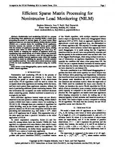
We consider a classic benchmark problem in computational fluid dynamics: the liddriven cavity flow (fig 1). The choice of the benchmark is motivated by its mathematical features that typically need a careful treatment in the framework of projection based parametric reduced order modeling, like nonlinearity and non-convexity [59]. Therefore it can be considered as a minimal working example to showcase the features of the sparse subspace learning approach. In particular we consider low Reynolds steady laminar flow governed by the equations : µ u · ∇ u − ∆u + ∇ p = 0 , (15) ∇·u=0 13
ux = 16x2 (1 uy = 0
x)2
y=1
ux , u y = 0
y=0 x=0
y
ux , u y = 0
ux , u y = 0
x=1
x
Figure 1: Schematics for the 2D lid driven cavity flow. with u(x, µ) and p(x, µ) being the velocity and pressure fields and µ = ρVη L being the Reynolds number. For this problem we seek a numerical approximation for u(x, µ), (x, µ) ∈ [0, 1]2 × [0, 1000]. 2.4.1
Deterministic solver
For a given choice of the Reynolds number the flow is solved with a high order mixed finite element formulation [60]. A cartesian mesh of 40 elements per direction is used. The nonlinearity is handled using a pseudo-transient method. Starting from an initial guess, that can be the corresponding Stokes flow for example, equation are integrated in time using a stable time-stepping algorithm until the steady state. Convergence is assessed using by checking the relative residual norm of eq. (15) and the `2 norm of the difference of the velocity field between two successive iterations. 2.4.2
Choice of the parametric basis
In low Reynolds number regime it can be reasonably assumed that the flow is laminar and that the solution of the equations (15) varies smoothly with the parameter µ. In this case we can adopt a high order polynomial basis to represent u(x, µ) in the parametric space for Reynolds numbers M ≡ [0, 1000]. When using polynomial approximation an optimal choice for the sampling is defined by the set of Gauss-Chebychev-Lobatto (GCL) points 1000} if k = 0 {0, (k) o n P ≡ 2 j−1 k−1 (0) µ j = 500(cos( k ) + 1)∀ j = 1, . . . , 2 ∪P if k > 0 2 The corresponding parametric basis is constructed using hierarchical Lagrangian inter-
14
R
S
M
0 50 100 150 200
=
250 300 350 400 450 500 0
50
100
150
200
250
300
350
400
450
500
nz = 88405
Figure 2: Heatmap plot showing the magnitude of both sampling points Mi j and representation coefficients S i j , evidencing the sparsity of the solution of the parametric lid-driven cavity flow in the space spanned by hierarchical polynomial function. The block triangular structure of the matrix R is also shown. polation. For a given hierarchical level k and Nµ(k−1) < j ≤ Nµ(k) : ψ j (µ) ≡ L(k) j (µ) =
Y µi ∈P(k) \µ j
2.4.3
µ − µi µ j − µi
∀µ j ∈ H (k)
Results
In order to get better insight on the structure of the sparse representation of the solution in the parametric space, algorithm 1 is run first without adaptiveness in the sampling. Figure 2 shows a heatmap plot of the elements in the representation S and measurements M matrices to give a qualitative visualization of the sparsity of the of first with respect to the second. Indeed, more than half of the elements in S can be pruned without significant effect on the solution, that is with a relative approximation error less than 10−6 . The same figure shows the block diagonal structure of the interpolation operator R obtained from the quasi-interpolative feature of the hierarchical polynomial basis used in this example. As a second step we solve the same problem with adaptive sampling. This can be introduced in a straightforward and non-intrusive way. Indeed, most of well designed iterative solvers (linear and nonlinear) perform a check on the initial guess solution before actually start running. If the convergence criterion is already met by the first attempt solution, the solver does not perform any iteration and returns the initial guess ¯ ij as the correct solution. Following this rationale, the predictions from hierarchical M interpolation offers an optimal initial guess to initialize the deterministic solver at a new sampling point. If this solution is good enough the solver is not run and the corresponding surplus coefficient is automatically set to zero. This strategy avoids the delicate task of defining a specific error estimation approach for each new problem by leaving this issue to the deterministic solver which can be therefore easily plugged in the SSL algorithm. Running algorithm 2 confirms this idea. In figure 3 we report the magnitude of the hierarchical surpluses as a function of the simulation number (simulation are ordered in the sense of hierarchical levels). These decay very fast until 15
10
-5
ks(µj )k1
ErrorEstimator
10
0
10-10
10
-15
10-20
0
100
200
300
400
500
600
Simulation
j
Figure 3: The norm of the sparse surplus functions s(x, µ j ) decreases with the refinement in the parametric space. The stagnation observed is due to the fact that the convergence tolerance in the direct solver is set to 10−8 , while the point with zero (to the machine precision) surplus coefficients correspond to the simulations that were skipped by the adaptive algorithm. they reach a plateau around the level of 10−8 . This phenomenon is explained by the fact that convergence criterion tolerance was set to this value, therefore the presence of the plateau indicates that the parametric sampling reached the level of precision of the direct solver. The points that are set to zero (to the machine precision) correspond to the cases where the adaptive algorithm skipped the solution and automatically set the corresponding surplus to zero. In this case, more than half of the solution were not computed at all. As the parametric sampling is refined, the sparse surplus coefficients S i j converge ¯ i j becomes an increasingly better initial guess for Mi j . This imand the prediction M plies that the convergence in the parametric space also accelerates the convergence on the deterministic iterative solver which require less and less iterations to reach convergence. To quantify this idea, we represented a measure of the computational work associated to each direct solution performed by the solver as a function of the magnitude of the surplus coefficients, figure 4. We assume, as a measure of the computational work, the number of iterations required by the pseudo-transient solver to converge to the steady state. In this way we make this measure platform independent. In figure 4 the surplus coefficients are shown to be linearly correlated to the computational work in the asymptotic convergence regime. Since polynomial approximation guarantees exponential convergence of the S i j coefficients, the linear decay of the computational work with the surplus coefficients implies that even though the number of sampling points increase the overall computational work per hierarchical level decreases. The numerical rank obtained in the final approximation using a tolerance of 10−7 in the irsvd algorithm is r = 9. Both space functions and parameters functions are represented in figure 5. For further details see appendix A.
16
106
10
Level 0 Level 1 Level 2 Level 3 Level 4 Level 5 Level 6 Level 7 Level 8 Level 9
5
Wj
104 103 102 101 100 10-10
10-5
100
105
ks(µj )k1
Figure 4: The surplus norm of surplus functions s(x, µ j ) correlates linearly with the amount of computational work W j required to compute direct solutions Mi j using the ¯ i j as initial guess in the nonlinear solver. The computational work is predictions M measured by the number of nonlinear iterations required by the direct solver to compute a solution. Since the computational work decays linearly with the magnitude of the surplus functions, and the latter decays exponentially with the order of the spectral approximation, we observe that the overall computational work per hierarchical level decreases when the hierarchical sampling reaches its asymptotic convergence regime.
3
Time dependent models
Parametric solutions of transient, or pseudo-transient, models can also be computed in the SSL framework. A first possibility consists in considering a space-time discretization uh (x, t, µ) :=
Nµ N s Nt X X
S i j φi (x, t)ψi (µ) ,
(16)
i=1 j=1
in which the set of functions φi (x, t) forms a representation basis in the space-time domain, (x, t) ∈ Ω × [0, T ]. This allows applying exactly what has been described in section 2. In particular, a subspace for the hierarchical surpluses may be found as shown in section 2.3. An alternative approach consists in splitting space and time into separated dimensions, which yields: uh (x, t, µ) :=
Nµ Ns X Nt X X
S i jk φi (x)ϕ j (t)ψk (µ) ,
(17)
i=1 j=1 k=1
where the set of functions φi (x), ϕ j (t) and ψk (µ) form a representation basis in the physical space x ∈ Ω, time interval t ∈ [0, T ] and parametric space µ ∈ M, respectively. The scalars S i jk are representation coefficients forming a third-order tensor. Both Eq. (16) and (17) are in principle equivalent, as they yield a total complexity of N s × Nt × Nµ . However, Eq. (17) allows seeking for a tensor subspace, which is 17
2
3
4
5
6
7
8
9
1.2
3
1 0.8
6
1
4
8 2
0.6 0.4
R i(Re)
Parametric Functions Ri (µ)
Space Functions vi (x)
1
9
0.2 0 7
-0.2
5
-0.4 -0.6 -0.8
0
200
400
600
800
1000
Re
Figure 5: Sparse Subspace Learning solution for the parametric lid-driven cavity steady state laminar flow for Reynolds number between 0 and 1000. The space modes are P given by vi (x) = n Uni φn (x). The first nine modes are visualized by streamlines and intensity of the corresponding field. The corresponding parametric functions are also P reported. These are defined as Ri (µ) = n Vmi ψm (µ). In this example the tolerance criterion used for the direct solver convergence was 10−8 , while the truncation criterion adopted for the determination of the numerical rank r in the irsvd algorithm is 10−7 . likely to be more compact in terms of representation than its matrix counterpart. We shall elaborate on the tensor subspace approach in next lines. For the sake of clarity, we shall denote a tensor with values in the field Kn1 ×n2 ×n3 either by |n1 ,n2 ,n3 (the first time it is introduced) or simply , in subsequent appearances. Suppose that the hierarchical collocation approach allowing for a sampling of the
18
parameter domain is applied exactly in the same manner as described in section 2. As a result, we get a three-dimensional tensor |n1 ,n2 ,n3 , containing the hierarchical surpluses, where n1 is typically the number of degrees of freedom related to the space discretization, n2 is the number of time steps and n3 is the total number of collocation points at convergence. We seek a tensor decomposition of rank-(r1 , r2 , r3 ) given by =
r3 r1 X r2 X X
σi jk ui1 ⊗ u2j ⊗ uk3 ,
(18)
i=1 j=1 k=1
which using the tensor multiplication [[25], sec. 2.5], can also be written as follows: = ×1 U1 ×2 U2 ×3 U3 ,
(19)
where the factor matrices U1|n1 ×r1 , U2|n2 ×r2 and U3|n3 ×r3 are usually orthonormal and define linear transformations in each direction. They can be regarded as the singular vectors in each direction. On the other hand, |r1 ×r2 ×r3 is called the core tensor, and its entries express the level of interaction between the different singular vectors. A tensor decomposition such as Eq. (19) is usually computed with the hosvd algorithm [61], based on the application of the svd on successive matricizations of the original data. Briefly: S(d) = Ud Σd V∗d ,
d = 1, 2, 3.
(20)
The core tensor is computed: Σ(d) = Σd V∗d (U1 ⊗ · · · ⊗ Ud−1 ⊗ Ud+1 ⊗ · · · ⊗ UD ).
(21)
Which in our case means that the core can be computed either as Σ(1) = Σ1 V∗1 (U2 ⊗ U3 ), Σ
(2)
=
Σ
(3)
=
Σ2 V∗2 (U1 Σ3 V∗3 (U1
⊗ U3 ),
(22) or
⊗ U2 ).
(23) (24)
Applying the hosvd may be expensive in terms of both memory requirements and computational cost, especially if the input data does not fit in fast memory. For this reason, we propose to replace the standard svd by the the irsvd, already presented in section A.2. In this manner, the factor matrices can be updated in order to account for the data stream.
3.1
Application to Sheet Metal Forming Simulation
In this example we apply SSL to transient stamping simulation of a hotformed automotive b-pillar. The objective is to assess the process sensitivity to the friction between the metal blank and the stamping tooling (punch and dye). Then numerical solution is sought in Ω × T × M, where the space domain Ω is shown in figure 6, the time interval is defined as T ≡ [0, 8][s] and M ≡ [0.05, 0.3] is the parametric space of friction coefficients. Frictional contacts are modeled using Coulomb’s friction law. Direct simulations were run on 4 hierarchical levels using the commercial software PamStamp 2G. The metal blank is modeled using quadrilateral shell elements with 1.5mm 19
initial uniform thickness. The stress-strain relation for steel is modeled by means of Krupkowsky’s law taking into account the strain hardening during the metal forming process. The punch and the dye are assumed as rigid elements. From each simulation we export displacements, plastic strain, thickness and thinning fields, each requiring a separate tensor approximation. For the displacement field, for instance, the final solution numerical rank is (6, 5, 3), ensuring reasonable accuracy for this application (less than 1% error on the predicted displacement). Other fields produce similar results. Figure 6 shows space, time and parametric modes for the displacement field, while three particular solutions for the thinning are shown in figure 7.
4
Extension to high-dimensional parametric problems
In higher dimensional problems the extension of hierarchical sampling is non trivial. Sampling high-dimensional spaces using the strategy described so far is limited by the curse of dimensionality. Indeed, the sampling points at a hierarchical level k would be simply given by the tensor product of point samplings P(k) d along each dimension d. Assuming D dimensions, this writes: (k) P(k) = P1(k) ⊗ P(k) 2 ⊗ . . . PD ≡
D O
P(k) d
d=1
Given that each point set is the union of all previous hierarchical refinements P(k) d =
k [
Hd(h) ,
h=0
The D-dimensional hierarchical refinement given by the tensor product rule would be : O D D D [ O (k) (k−1) H (k) ≡ P(k) \ P(k−1) = H P Hd(k) ∀k ∈ N+ ⊗ ∪ h d h=1
d=1 d,l
d=1
The tensor product rule implies that hierarchical refinements grow exponentially with the dimension D of the problem. To alleviate this issue we adopt Smolyak’s rule to construct higher dimensional refinement sets [62]. This replaces the traditional tensor product rule by the following expression: H (k) ⊃ H s(k) =
D [ O
Hd(hd ) , ∀k ∈ N+
(25)
|h|1 =k d=1
with h ≡ {h1 , . . . , hd , . . . , hD }. The complexity Smolyak’s rule grows polynomially with the dimensionality of the parametric hypercube, instead of exponentially, while retaining the same accuracy on the approximation of the function, provided that the high order mixed derivatives are bounded [46]. Therefore the method is not subject to 20
Frontal
Lateral Die Punch
(a) Mode 1
0.4 0.4 0.2 0.2 0 0 0.2 0.2 0.4 0.4 0
(b) Mode 2
Mode 1 Mode 2 Mode 1 Mode 2 Punch stroke (mm) 80 Punch 60 stroke 40 (mm) 20 0 80 60 40 20 0
2
0
4 6 2Time 4(sec) 6 Time (sec)
Mode 3 Mode 3 0.4 0.4 0.4 0.2 0.2 0.20 0 0 0.2 0.2 0.2 0.4 0.4
0.4
8
(c) Mode 3
8
Mode 4 Mode 4
0.1 0.2 0.3 0.1 coefficient 0.2 (-) 0.3 Friction 0.1 0.2 0.3 Friction coefficient (-)
(b) Parameter modes (-) Friction coefficient
(a) Time modes (a) Time modes
(b) Parameter modes
Figure 6: Order reduction of the stamping solution: normalized space, time and parameter modes of the displacement field. Figure 7: First four normalized time modes of the displacement field. Figure 7: First four normalized time modes of the displacement field. the curse of dimensionality at least in the space of smooth functions. This concept Time has D-dimensional refinement given grid by the tensor product rule beenThe successfully used hierarchical in the framework of sparse interpolation and quadrature be : The hierarchical refinement given by hierarchical the tensor product rule and [63],would withD-dimensional a variety of different basis functions including polynomials 2 3 would be : wavelet functions [64] and extended to dimensionally strategies [65]. Note D D D 3adaptive [ O O 62 (k) norm (k 1) 7 (k) (k) the(k) (k 1)for a different + that changing ` norm in equation (25) different samH ⌘ P 1\ P = [ 8k 2 N D4Hh ⌦ O DPd DHd yields 5[ O (k 1) 7 (k) (k) (k 1) h=1 6 (k) d=1 + d=1 pling strategies. Using the infinity (maximum norm) the classical tensor-product H(k) ⌘ P \P = norm H ⌦ P [ H 8k 2 N 4 h d6=l 5 d d h=1
d=1 d6=l
d=1
Friction coefficient
The tensor product rule implies that hierarchical refinements grow exponentiallyThe with the dimension D implies of the problem. To alleviate this issue weexponenadopt tensor product rule that hierarchical refinements grow 21 Smolyak’s construct D higher dimensional refinement sets [Smolyak]. tially withrule thetodimension of the problem. To alleviate this issue we This adopt replaces the rule traditional tensorhigher product rule by the following sets expression: Smolyak’s to construct dimensional refinement [Smolyak]. This replaces the traditional tensor product rule by the following expression: D [ O (hd ) (k) (k) H Hs = , 8k 2 N+ (17) DHd [ O (hd ) (k) (k) |h| =k d=1 H Hs = 1 Hd , 8k 2 N+ (17)
with h ⌘ {h1 , . . . , hd ,|h| . .1.=k , hDd=1 }. Smolyak hierarchical refinement grow subexponetially scaleshierarchical as o(N log(N )D 1 ) instead ND with h ⌘and {h1the , . . .problem , hd , . . . ,complexity hD }. Smolyak refinement growofsubexD 1 while retaining accuracy on the approximation of) the )function, proponetially and the the same problem complexity scales as o(N log(N instead of ND
Friction coefficient
Time
Figure 7: The figures shows the solutions for three different friction coefficients 0.05 (top), 0.175 (middle) and 0.3 (bottom) at times t = 2.32 s (left), t = 5.41 s (center) and t = 8.50 s (right). sampling is obtained. An alternative approach is represented by the hyperbolic-cross sampling [66].
4.1
Application to Stokes flow around parametric NACA four digits airfoil
In this section we show an application of the Sparse Subspace Learning method to the problem of steady state viscous incompressible and inertialess flow around a NACA four-digits airfoil. The geometry of the airfoil is known in analytical closed form as a function of four parameters: the chord c, the maximum thickness t, the maximum camber m and the position of maximum camber as a fraction of the chord p. In dimensionless form, the problem only depend on three parameters if the chord is chosen as reference unit length. Therefore the parametric solution of this problem is sought in the three-dimensional space {t, m, p} ∈ [0.06, 0.15] × [0, 0.1] × [0.34, 0.5]
22
reference
mapping
deformed
Figure 8: Airfoil shape variation with respect to a reference shape (NACA 0012 airfoil) are take into account by deforming a reference triangular mesh (leftmost panel). The nodes in the original mesh are moved according to a displacement field u solution of the elliptic problem (27) with imposed Dirichlet boundary condition prescribing the right shape on the airfoil boundary (central panel). An exemple of a typical mesh is shown in the rightmost panel. The velocity and pressure fields are governed by Stokes equations: ∆v − ∇p = 0 ∇ · v =0
(26)
paired with appropriate boundary condition prescribing no-slip at the airfoil boundary v(x = xb ) = 0 and uniform asymptotic velocity v∞ = cos(α)i + sin(α)j; with the angle of attack α = 10◦ for this case. The airfoil shape variation is taken into account through the mapping x(x0 ) = x0 + u(x0 ) where x0 is the coordinate in a reference (undeformed) domain, x is the physical coordinate in the transformed domain and u is a displacement field. In practice the mapping is found through the solution of the elliptic problem for the u: c1 u + c2 ∆x0 u + c3 ∇x0 [∇x0 · u] = 0
(27)
with prescribed Dirichlet boundary conditions on the airfoil boundaries in order impose the correct shape to the deformed domain. The subscript x0 indicates that the derivatives are taken with respect to the coordinates in the reference domain. The reference shape is chosen as the symmetric profile NACA 0012. The reference domain is then meshed using triangular elements. Equation (27) is solved on this domain to find the mapping u corresponding to a given shape of the family NACA 4-digits airfoils and the reference mesh is deformed accordingly, as shown in figure 8. The coefficients appearing in this equation are chosen on empirical basis as c1 = 50, c2 = 1, c3 = 24.5. The values are selected in order to avoid severe distorsion of the mesh. The Stokes problem is then solved on the deformed mesh using Crouziex-Raviart mixed finite elements formulation. There are two bottlenecks associated to this problem in the framework of projection based parametric reduced order modeling:
23
sparse sampling
full sampling
sparse adaptive sampling
0.5
0.5
0.45
p
p
0.45
0.4
0.4
0.35
0.35
0.1 0.05
m
0
0.06
0.08
0.1
t
0.12
0.14
0.1 0.05
m
0
0.06
0.08
0.1
0.12
0.14
t
Figure 9: Comparison between tensor product sampling strategy (leftmost panel), sparse grid sampling using Smolyak’s rule (central panel) and sparse adaptive sampling (rightmost panel). Note how the sampling along p is automatically refined in proximity of the values m = 0.1. This is because for m = 0 (symmetric profile) the position of maximum camber p does not affect the shape profile. On the contrary for cambered airfoils the value of the parameter p has a strong effect on the shape and therefore on the flow solution, therefore more sampling points are needed in this region. • The parametric mapping u(x0 , t, m, p) needs to be determined from the solution of equation (27). The difficulty in this step is associated to the parametrization of the Dirichlet boundary conditions describing the airfoil shape that are not expressed in a tensor format and an approximate decomposition must be sought. • Even if a separated variable approximation of u(x0 , t, m, p) can be obtained with reasonable accuracy, the weak form associated to problem (26) is not necessarily affine with respect to parameters {t, m, p}. A strategy to recover affine approximations in terms of geometrical parameters can be found in [67]. In this case the use of collocation does not require an affine approximation of the linear operators arising from the problem discretization, since the proposed method only relies on the output of the deterministic solver. This takes values of {t, m, p} as input and computes the Stokes flow around the corresponding airfoil using a triangular mesh generated through equation (27). A sparse and low rank approximation of both the flow solution and the mapping are constructed simultaneously. The sampling algorithm is run until all hierarchical surpluses fall below 10−8 and the truncation threshold for the rank was taken as 10−15 . In figure 9 we present a comparison between three possible sampling strategies. With respect to classical tensor product of 1D sampling points, Smolyak’s rule requires only a 0.6% of all points and adaptive Smolyak’s rule only 0.03%. The final solution approximate rank (for the prescribed precision) is 16. To assess the validity of the solution we compared results of the reduced parametric model to the results of the direct solver for some parameter combinations giving specific airfoils in the NACA 4-digits family. Results are presented in figure 10 and confirm that the accuracy of the model is around 10−8 . Note that error is sensibly smaller close to the location of the sampling points.
24
NACA 2412
NACA 6409
NACA 6515
NACA 6406
Figure 10: Error maps of the reduced order parametric solution with respect to direct solutions for specific airfoils shapes of the NACA four-digits family. The error is globally around 10−8 everywhere in the parametric space except in proximity of the collocation points where the error is remarkably smaller.
25
4.2
Application to crash simulations
A 64 Km/h
[mm]
Rigid Obstacle
B
C
D
Figure 11: Parametric simulation of the crash model for the NCAP Offset Deformable barrier frontal impact test. Final deformation corresponding to different combination of the parameters : (A) µ1 = 2.34 mm, µ2 = 2.09 mm, µ3 = 2.362.34 mm, µ4 = 1.61 mm; (B) µ1 = 3.74 mm, µ2 = 2.09 mm, µ3 = 3.78 mm, µ4 = 1.61 mm; (C) µ1 = 3.74 mm, µ2 = 0.84 mm, µ3 = 3.78 mm, µ4 = 0.64 mm; (D) µ1 = 2.34 mm, µ2 = 0.84 mm, µ3 = 2.34 mm, µ4 = 0.64 mm. Parametric modeling is of capital importance in simulation based engineering applications such as process and product optimization, identification, control and uncertainty quantification. Reduced order modeling offers a practical way to alleviate the curse of dimensionality that is inevitably encountered in high-dimensional parametric problems. In industrial practice the need of simulation code certification has somehow slowed down the process of integrating high fidelity simulation software with reduced order modeling tools. This is partly due to the intrusiveness of most of reduced order modeling approaches, which inevitably require modification of the original code to a certain extent. In this last section we show the results of parametric crash simulations performed using the commercial code Pam Crash. The reason behind the choice of this problem is very well related with the intrusiveness issue. In crash simulation, parametric modeling is extremely important in order to have a quick assessment of parameter sensitivity and performance/safety estimators before the actual physical model is built and tested. 26
The “digital twin” approach is a cost-wise efficient way to have a quick sweep of the parameter state space and identify the optimal configurations in the pre-design step. These will be eventually verified using high performance simulation and ultimately certified by experimental testing. Crash simulation code include binary actions that are external to the core PDE solver, such as plasticity or contact detection. In particular the last is extremely time consuming and can take up to 90% of the simulation time. In general such “control actions” are present in most simulation software, which is seldom limited to a simple core PDE solver. Traditional reduced order modeling requires a redefinition of the control actions. For instance the very concept of contact detection changes when the problem is formulated in terms of a reduced basis with global support, due to the intrinsically local nature of contacts. A non-intrusive approach allows to leave control actions to a lower level, inside the deterministic solver, since the reduced parametric model is built only on the solver output. For the same reason, it is also possible to build reduced models for specific quantity of interests extracted from simulation results. In the example reported in this section, crash simulations were run using the commercial software Pam Crash. The tested configuration correspond to the NCAP Offset Deformable barrier frontal impact, shown in figure 11. The car is driven at 64km/h and with 40% overlap into a deformable barrier which represents the oncoming vehicle. The test replicates a crash between two cars of the same weight, both travelling at a speed of 50km/h. In particular safety can be assessed with respect to the geometrical parameters in the model. In this case we considered four parameters, µ ≡ {µ1 , µ2 , µ3 , µ4 }, corresponding to the thicknesses of different parts (inner rail, outer rail, lower-outer rail and front frame). The reduced parametric displacement field is sought in the tensor form uh (x, t, µ) =
rµ rs X rt X X
Ci jk φi (x)ϕ j (t)ψk (µ) ,
(28)
i=1 j=1 k=1
Simulation were scripted using Python and a Matlab generic interface was used to recover the simulation results and build the reduced model. Globally, 401 simulations were run in parallel, each taking approximately one hour on 32 cores. The final deformations corresponding to different choices of the parameters are shown in figure 11. The model was exported using the pxdmf format for canonical tensor representations developed in the framework of PGD [68]. This allows the visualization and the post-processing of the solution in real time using open source software Paraview. This solution can be easily explored for sensitivity analysis or uncertainty quantification with respect to the parameters.
5
Concluding remarks
We showed the application of hierarchical adaptive sampling in the parametric space combined with an incremental tensor approximation technique in order to learn the 27
low-rank and sparsity features characterizing the solution of parametric models. We tested the proposed approach through numerical experimentation on different models, including time dependent and multi-parametric problems. Results show that the collocation strategy can be easily integrated with existing deterministic solvers in a nonintrusive way, as the method does not require access and manipulation of the solver internal operators or routines. This feature enables reduced order modeling for problems which are not straightforwardly compatible with traditional projection-based approaches requiring the appropriate format in the problem setting. Approximating a parametric solution in explicit form not only requires the construction of a reduced basis but also the determination of the parametric modes. When these have a sparse representation, the number of coefficients needed to accurately describe the functional dependency of the solution in the parametric space is typically small, although this is in general higher than the numerical rank of the approximation. Therefore, in agreement with other studies [69], we observed that if the number of direct runs sampling is fixed, the offline/online approach yields a more accurate solution (when the structure of the problem makes it possible) than an explicit offline solution. However, as pointed out in [70], in many applications the hierarchical collocation approach is sufficient to have reasonable accuracy for an explicit representation of the solution, or a given quantity of interest, without the need of solving a reduced system each time a new query is demanded. In many engineering applications, the proposed approach is particularly suitable for delivering fast performance estimators, allowing for quick parametric sweeps so as to assess sensitivity with respect to the parameters, find optimality or evaluate and quantify uncertainty in the data.
Acknowledgments The authors of the paper would like to acknowledge Jean-Louis Duval, Jean-Christophe Allain and Julien Charbonneaux from the ESI group for the support and data for crash and stamping simulations.
A
Incremental Random Singular Value Decomposition
A.1
Randomized singular value decomposition
Suppose we are given the input data matrix S, which in our case contains the hierarchical surpluses, and assume that a rank-r approximation like in Eq. (7) wants to be computed. There are two main ideas behind the rsvd: • The first is to realize that a partial SVD can be readily computed provided that we are able to construct a low-dimensional subspace that captures most of the range of the input data matrix. • The second is to observe that such low-dimensional subspace can be computed very efficiently using a random sensing method.
28
Let us start with the first of the aforementioned ideas. Suppose that we are given a matrix Q|m×p with r ≤ p � n orthonormal columns such that the range of S is well captured, i.e.: kS − QQ∗ Sk ≤ ε,
(29)
for some arbitrarily small given tolerance ε. Then, the input data is restricted to the subspace generated by its columns, that is: B|p×n = Q∗ S. Observe at this point that we implicitly have the factorization A ≈ QB. Next, we compute an SVD factorization of ˜ Σ˜ V ˜ ∗ , where factors are defined as U ˜ |p×p , Σ˜ |p×p and V ˜ |n×p . This operthe matrix B = U ation is much less expensive than performing the SVD on the initial data set because the rank is now restricted to the rows of B. Finally, in order to recover the r dominant ˜ Σ = Pt ΣP ˜ and components, we define an extractor matrix P|p×r and set: U = QUP, ˜ V = VP. In summary, given Q, it is straightforward to compute a SVD decomposition at a relatively low cost O(mnp + (m + n)p2 ). Now we address the second question, that is, how to compute the matrix Q. We first draw a random Gaussian test matrix, Ω|n×p . Then, we generate samples from the data matrix, i.e. Y|m×p = AΩ. Observe that if the rank of input data matrix was exactly r, the columns of Y would form a linearly independent set spanning exactly the range of S, provided that we set p = r. Since in general the true rank will be greater than r, we must consider an oversampling parameter by setting p = r + α. This will produce a matrix Y whose range has a much better chance of approximating well the range of the input data matrix. Finally, Q can be obtained from the orthogonalization of Y. In fact, it can be shown that the following error bound is satisfied i h p (30) kS − QQ∗ Sk ≤ 1 + 9 p min{m, n} σr+1 , with a probability in the order of O(1 − α−α ). That is, the failure probability decreases superexponentially with the oversampling parameter [52]. Remark 1 (On the optimal decomposition) Observe that the standard SVD produces Q|m×r such that kS − QQ∗ Sk = σr+1 , but at a higher cost O(mn min{m, n}). A prototype version of the randomized SVD is given in the Algorithm 4. Neglecting the cost of generating the Gaussian random matrix Ω, the cost of generating the matrix Q is in the order of O(mnp + mp2 ) flops. In consequence, the computational cost of the entire rsvd procedure remains as O(mnp + (m + n)p2 ). The algorithmic performance of the rsvd can be further improved by introducing a number of refinements at the price of worsening slightly the error bounds. In particular, the most expensive steps in the rsvd algorithm consist in forming matrices Y and B, which require in the order of O(mnp) flops. The first can be reduced to O(mn log(p)) by giving some structure to the random matrix Ω, while the second can be reduced to O((m+n)p2 ) via row extraction techniques, which leaves the total cost O(mn log(p) + (m + n)p2 ). The interested reader can find further details on these refinements as well as on their impact on the assessment in [52]. 29
Algorithm 4 Randomized singular value decomposition: rsvd Require: S|m×n , r, α . Data matrix, rank and oversampling parameter Set p = r + α 1: Draw Ω|n×p . Random Gaussian test matrix 2: Generate samples Y|m×p = SΩ 3: Compute Q|m×p = orthogonalize(Y) . Captures range of S 4: Restrict B|p×n = Q∗ S ˜ |p×p , Σ|p×p , V|n×p ] = svd(B) 5: Compute [U . Standard deterministic SVD ˜ 6: Set U|m×p = QU return U|m×r , Σ|r×r , V|n×r . Retain r first components
A.2
Incremental randomized singular value decomposition
In this section we present an incremental variant of the randomized SVD algorithm, discussed in section A.1. The objective is twofold: (i) to be able to learn a subspace for the hierarchical surpluses as they are streamed from the sparse sampling procedure; (ii) to perform it at a computational cost that scales reasonably with the number of samples. Let us assume that we want to compute a rank-r approximation of some streamed data, and that we have chosen an oversampling parameter α such that p = r + α, as in section A.1. Let us denote by S0|m×n the old data matrix, whereas S|m×n0 is the new data columns such that the total data is now S1|m×(n+n0 ) = [S0 | S]. We would like to compute an approximated SVD decomposition S1 ≈ U1 Σ1 V∗1 at a cost which is roughly independent on n, the number of columns of the old data. For the sake of completeness, recall that U1|m×p , Σ1|p×p and V1|(n+n0 )×p . In order to do so, suppose that we are given a non-truncated SVD approximation of the old data, i.e. S0 ≈ U0 Σ0 V∗0 , with U0|m×p , Σ0|p×p and V0|n×p . Suppose that we also dispose of the matrix of random samples Y0|m×p . Then, in order to account for the new data we only need to generate a random Gaussian test matrix Ω|n0 ×p and perform a small product which only involves the new data: Y1 = Y0 + SΩ.
(31)
The matrix Q1|m×p can be obtained from the orthogonalization of Y1 at a cost that remains stable, as it does not depend on n nor n0 . Next, input data has to be restricted to the range of Q1 . Recalling that we already dispose of a non-truncated SVD approximation of the old data: # h i h i " V∗ 0 0 B1 ≈ Q∗1 U0 Σ0 V∗0 S = Q∗1 U0 Σ0 Q∗1 S , (32) | {z } 0 In0 ×n0 ˜ B
where In0 ×n0 is the identity matrix of size n0 . Similarly to section A.1, observe that Eq. ˜ Hence, if we compute a SVD decomposition of (32) yields a factorization S1 ≈ Q1 B. ˜ the factor B, ˜ 1V ˜ ∗, B˜ = UΣ
˜ |p×p , Σ1|p×p and V ˜ |(p+n0 )×p , with U
30
(33)
we can conclude the algorithm by setting: " # 0 ˜ and V1 = V0 ˜ U1 = Q 1 U V. 0 In0 ×n0
(34)
A prototype version of the incremental randomized SVD is given in the Algorithm 5. Algorithm 5 Incremental randomized singular value decomposition: irsvd Require: S|m×n0 , U0|m×p , Σ0|p×p , V0|n×p , Y0|m×p . Streamed data, old factors and old samples 1: Draw Ω|n0 ×p 2: Correct samples Y1|m×p = Y0 + SΩ 3: Compute Q1|m×p = orthogonalize(Y1 ) i h ˜ |p×(p+n0 ) = Σ0 U∗ S 4: Form B 0 ˜ |p×p , Σ1|p×p , V ˜ |(p+n0 )×p ] = svd(B) ˜ 5: Compute [U 6: Set U1|m×p and V1|(n+n0 )×p as indicated in Eq. (4) return U1 , Σ1 , V1 and Y1 . Do not truncate: retain all p components Observe that the cost of the irsvd algorithm is driven by O((m+n)p2 ) when choosing n0 ∼ p, while if one chooses n0 � p, the cost matches the standard rSVD, that is O(mn0 p). A more detailed analysis of the flop count indicates that in fact, the only dependence on n of the algorithm is due to the cost of updating the right singular vectors in Eq. (34). On the other hand, the reader should keep in mind that, for the applications targeted in this paper, the number of rows of the input dataset (degrees of freedom after discretization of a PDE) is at least one or two orders of magnitude bigger than the number of columns (solution snapshots). As a consequence, the cost of the irsvd turns out to be roughly independent on n. A final consideration that should not be neglected is that, for data sets that do not fit in the core memory, the cost of transferring data from slow memory dominates the cost of the arithmetics. This can be generally avoided with the incremental algorithm presented in this section.
A.3
A numerical example: order reduction applied to the lid-driven cavity problem
In this section, we provide numerical evidence on the performance of the irsvd, as described in section A.2. In particular, we apply irsvd on the set of hierarchical surpluses, Sldc , coming from the solution of the lid-driven cavity problem, as described in 2.4. The size of the data matrix is m = 14, 082 rows and n = 513 columns. An overkill value of the oversampling parameter is taken, α = r (i.e. p = 2 r). Firstly, we show that the low-rank singular value decomposition given by the irsvd tends to both the standard svd and the rsvd as the number of processed columns approaches the number of columns of the entire dataset. To that end, we choose a rank r = 20 and a fixed bandwidth n0 = 5. Figure 14 shows the evolution of the singular values as the number of processed columns increases. It can be noticed that, in fact, after a relatively low number of columns are processed (say 20), the singular values are 31
already very close to the reference ones. This is simply because when coupling irsvd with the hierarchical sampling the surpluses that come from higher hierarchical levels are naturally associated to the first singular vectors. On the contrary, lower hierarchical levels yield smaller surpluses, as the hierarchical sampling method converges. When the entire dataset is processed, the irsvd yields a SVD that matches the standard one, see Figure 12f. In order to further assess the convergence of the irsvd towards the standard svd decomposition, the energy error between both decompositions is measured: sP r 2 i=1 (σirsvd − σsvd ) , (35) εr = Pr 2 i=1 σsvd for a given rank r. Figure 13 shows the evolution of εr for several bandwidth. It can be observed that the bandwidth hardly influences the convergence results. Next, the computational cost of the irsvd must be assessed. Figure 14a shows the runtime (denoted by τ) of the irsvd, i.e. Algorithm 5, as a function of the bandwidth. The runtime is computed as the average of three executions. Results confirm that, as discussed in section A.2, the computational cost is independent on the bandwidth size. Besides, it can be observed that greater ranks yield greater runtimes. In fact, the computational complexity should depend quadratically on the rank. This quadratic scaling is confirmed by Figure 14b, which shows the normalized rank r˜ = r/r0 (with r0 = 10) against the normalized runtime τ˜ = τ/τ0 , where τ0 is the runtime associated to r0 . It can be seen that for all bandwidth the normalized runtime scales super-linearly with the normalized rank (linear scaling is depicted for reference). Finally, it is worth to highlight that in many practical applications the cost of irsvd turns out to be independent on n, the total number of columns of the data set. This is simply because usually m � n and then the computational complexity reduces to O(mp2 ). In other words, the cost only starts being influenced by n when n ∼ m. Figure 15 shows the runtime of each irsvd call, averaged over three runs. For the sake of clarity, runtimes have been normalized to their mean value, while the vertical axis scale is chosen so we can observe ±50% deviations from the mean. Results show that runtime deviates very few from the mean. Moreover, the cost of each call remains fairly constant as the number of processed columns increases, which confirms the discussion above.
References [1] F. Zorriassatine, C. Wykes, R. Parkin, and N. Gindy. A survey of virtual prototyping techniques for mechanical product development. Proceedings of the Institution of Mechanical Engineers, Part B: Journal of Engineering Manufacture, 217(4):513–530, 2003. [2] J.T. Oden, T. Belytschko, J. Fish, T.J.R. Hughes, C. Johnson, D. Keyes, A. Laub, L. Petzold, D. Srolovitz, and S. Yip. Simulation-based engineering science: revolutionizing engineering science through simulation. Report of the NSF Blue
32
Ribbon Panel on Simulation-Based Engineering Science. National Science Foundation, Arlington, VA, 2006. [3] S.C. Glotzer, S. Kim, P.T. Cummings, A. Deshmukh, M. Head-Gordon, G. Karniadakis, L. Petzold, C. Sagui, and M. Shinozuka. International assessment of research and development in simulation-based engineering and science. Panel Report. World technology evaluation center, Inc., Baltimore, MD, 2009. [4] R.E. Bellman. Dynamic Programming. Courier Dover Publications, New York, republished edition, 2003. [5] D.C. Montgomery. Design and analysis of experiments. John Wiley & Sons, Hoboken, NJ, 8th edition, 2013. [6] E.K.P. Chong and S.H. Zak. An introduction to optimization. Wiley series on discrete mathematics and optimization. John Wiley & Sons, Hoboken, NJ, 4th edition, 2013. [7] A. Antoulas, D.C. Sorensen, and S. Gugercin. A survey of model reduction methods for large-scale systems. Contemp. Math., 280:193–220, 2001. [8] R.A. Bialecki, A.J. Kassab, and A. Fic. Proper Orthogonal Decomposition and Modal Analysis for acceleration of transient FEM thermal analysis. Int. J. Numer. Meth. Engng., 62(6):774–797, 2005. [9] A. Quarteroni, A. Manzoni, and F. Negri. Reduced Basis Methods for Partial Differential Equations: An Introduction. Modeling and Simulation in Science, Engineering and Technology. Springer, Basel, 1st edition, 2015. [10] D.B.P. Huynh, G. Rozza, S. Sen, and A.T. Patera. A successive constraint linear optimization method for lower bounds of parametric coercivity and infsup stability constants. C.R. Math., 345(8):473–478, 2007. [11] C. Daversin and C. Prud’homme. Simultaneous empirical interpolation and reduced basis method for non-linear problems. C.R. Math., 353(12):1105–1109, 2015. [12] M. Barrault, Y. Maday, N.C. Nguyen, and A.T. Patera. An “empirical interpolation method”: application to efficient reduced-basis discretization of partial differential equations. C.R. Acad. Sci. I-Math., 339(9):667–672, 2004. [13] C. Farhat, T. Chapman, and P. Avery. Structure-preserving, stability, and accuracy properties of the energy-conserving sampling and weighting method for the hyper reduction of nonlinear finite element dynamic models. Int. J. Numer. Meth. Engng., 102:1077–1110, 2015. [14] S. Chaturantabut and D.C. Sorensen. Nonlinear model order reduction via Discrete Empirical Interpolation. SIAM J. Sci. Comput., 32(5):2737–2764, 2010.
33
[15] M.A. Grepl, Y. Maday, N.C. Nguyen, and A.T. Patera. Efficient reduced-basis treatment of non-affine and nonlinear partial differential equations. ESAIM Math. Model. Num., 41(3):575–605, 2007. [16] Y. Maday, N.C. Nguyen, A.T. Patera, and S.H. Pau. A general multipurpose interpolation procedure: the Magic Points. CPPA, 8(1):383–404, 2009. [17] D. Ryckelynck. A priori hypereduction method : an adaptive approach. J. Comput. Phys., 202(1):346–366, 2005. [18] D. Amsallem and C. Farhat. An online method for interpolating linear parametric reduced-order models. SIAM J. Sci. Comput., 33(5):2169–2198, 2011. [19] J. Hern´andez, M.A. Caicedo, and A. Ferrer. Dimensional hyper-reduction of nonlinear finite element models via empirical cubature. Comput. Meth. Appl. Mech. Engrg., 313:687–722, 2017. [20] M.L. Rap´un, F. Terragni, and J.M. Vega. Lupod: Collocation in POD via LU decomposition. J. Comput. Phys., 335:1–20, 2017. [21] D. Kumar, M. Raisee, and C. Lacor. An efficient non-intrusive reduced basis model for high dimensional stochastic problems in CFD. Comput. Fluids, 138:67–82, 2016. [22] E. Pruli`ere, F. Chinesta, and A. Ammar. On the deterministic solution of multidimensional parametric models using the Proper Generalized Decomposition. Math. Comput. Simul., 81(4):791–810, 2010. [23] W. Hackbusch. Tensor spaces and numerical tensor calculus. Springer Series in Computational Mathematics. Springer-Verlag, Berlin-Heidelberg, 1st edition, 2012. [24] L. Grasedyck, D. Kressner, and C. Tobler. A literature survey of low-rank tensor approximation techniques. arXiv:1302.7121, 2013. [25] T.G. Kolda and B.W. Bader. Tensor decompositions and applications. SIAM Rev., 51(3):455–500, 2009. [26] A. Ammar, B. Mokdad, F. Chinesta, and R. Keunings. A new family of solvers for some classes of multidimensional partial differential equations encountered in kinetic theory modeling of complex fluids. Part II: transient simulation using spacetime separated representations. J. Non-Newtonian Fluid Mech., 144(2-3):98–121, 2007. [27] A. Nouy. A priori model reduction through Proper Generalized Decomposition for solving time-dependent partial differential equations. Comput. Meth. Appl. Mech. Engrg., 199:1603–1626, 2010.
34
[28] F. Chinesta, A. Leygue, F. Bordeu, J.V. Aguado, E. Cueto, D. Gonzalez, I. Alfaro, A. Ammar, and A. Huerta. PGD-based Computational Vademecum for efficient design, optimization and control. Arch. Comput. Methods Eng., 20(1):31–59, 2013. [29] F. Chinesta, P. Ladev`eze, and E. Cueto. A short review on model order reduction based on Proper Generalized Decomposition. Arch. Comput. Methods Eng., 18(4):395–404, 2011. [30] A. Ammar, F. Chinesta, P. D´ıez, and A. Huerta. An error estimator for separated representations of highly multidimensional models. Comput. Meth. Appl. Mech. Engrg., 199(25-28):1872–1880, 2010. [31] A. Uschmajew. Local convergence of the alternating least squares algorithm for canonical tensor approximation. SIAM J. Matrix Anal. Appl., 33(2):639–652, 2012. [32] C. Quesada, I. Alfaro, D. Gonzalez, E. Cueto, and F. Chinesta. PGD-based model reduction for surgery simulation: solid dynamics and contact detection. Lect. Notes Comput. Sc., 8789:193–202, 2014. [33] J.V. Aguado, D. Borzacchiello, Ch. Ghnatios, F. Lebel, R. Upadhyay, C. Binetruy, and F. Chinesta. A Simulation App based on reduced order modeling for manufacturing optimization of composite outlet guide vanes. Adv. Model. Simul. Eng. Sci., 4(1), 2017. [34] D. Borzacchiello, J.V. Aguado, and F. Chinesta. Reduced Order Modelling for efficient numerical optimisation of a hot-wall Chemical Vapour Deposition reactor. Int. J. Numer. Method H., 27(4), 2016, in press. [35] Ch. Ghnatios, F. Masson, A. Huerta, A. Leygue, E. Cueto, and F. Chinesta. Proper Generalized Decomposition based dynamic data-driven control of thermal processes. Comput. Meth. Appl. Mech. Engrg., 213-216:29–41, 2012. [36] A. Cohen and R. DeVore. Approximation of high-dimensional parametric PDEs. Acta Numer., 24:1–159, 2015. [37] M. Bachmayr, A. Cohen, and W. Dahmen. Parametric PDEs: Sparse or low-rank approximations? arXiv:1607.04444, 2016. [38] J.P. Boyd. Chebyshev and Fourier spectral methods. Courier Corporation, 2001. [39] E. Cand`es and J. Romberg. Sparsity and incoherence in compressive sampling. Inverse Probl., 23(3):969, 2007. [40] A. Gilbert and P. Indyk. Sparse recovery using sparse matrices. Proc. IEEE, 98(6):937–947, 2010. [41] D.L. Donoho. Compressed sensing. IEEE T. Inform. Theory, 52(4):1289–1306, 2006.
35
[42] S.S. Chen, D.L. Donoho, and M.A. Saunders. Atomic decomposition by basis pursuit. SIAM Rev., 43(1):129–159, 2001. [43] R. Tibshirani. Regression shrinkage and selection via the lasso. J. R. Stat. Soc. Series B Methodol., pages 267–288, 1996. [44] H. Zou and T. Hastie. Regularization and variable selection via the elastic net. J. R. Stat. Soc. Series B Stat. Methodol., 67(2):301–320, 2005. [45] S.L. Brunton, J.L. Proctor, and J.N. Kutz. Discovering governing equations from data by sparse identification of nonlinear dynamical systems. Proc. Natl. Acad. Sci. USA, 113(15):3932–3937, 2016. [46] H.J. Bungartz and M. Griebel. Sparse grids. Acta Numer., 13:147–269, 2004. [47] F. Nobile, R. Tempone, and C.G. Webster. A sparse grid stochastic collocation method for partial differential equations with random input data. SIAM J. Numer. Anal., 46(5):2309–2345, 2008. [48] D. Pfl¨uger, B. Peherstorfer, and H.J. Bungartz. Spatially adaptive sparse grids for high-dimensional data-driven problems. J. Complexity, 26(5):508–522, 2010. [49] T. Gerstner and M. Griebel. Dimension-adaptive tensor-product quadrature. Computing, 71(1):65–87, 2003. [50] F. Nobile, R. Tempone, and C.G. Webster. An anisotropic sparse grid stochastic collocation method for partial differential equations with random input data. SIAM J. Numer. Anal., 46(5):2411–2442, 2008. [51] G.H. Golub and C.F. Van Loan. Matrix computations. The Johns Hopkins University Press, Baltimore, MD, 3rd edition, 1996. [52] N. Halko, P.G. Martinsson, and J.A. Tropp. Finding structure with randomness: Probabilistic algorithms for constructing approximate matrix decompositions. SIAM Rev., 53(2):217–288, 2011. [53] R. A. Harshman. Foundations of the parafac procedure: Models and conditions for an “explanatory” multi-modal factor analysis. UCLA Working Papers in Phonetics, 1970. [54] J. D. Carroll and J. J. Chang. Analysis of individual differences in multidimensional scaling via an n-way generalization of eckart-young decomposition. Psychometrika, 35(3):283–319, 1970. [55] Y. Li. On incremental and robust subspace learning. 37(7):1509–1518, 2004.
Pattern recognition,
[56] H. Zhao, P. C. Yuen, and J. T. Kwok. A novel incremental principal component analysis and its application for face recognition. IEEE Transactions on Systems, Man, and Cybernetics, Part B (Cybernetics), 36(4):873–886, 2006.
36
[57] A. Sobral, C. G. Baker, T. Bouwmans, and E. Zahzah. Incremental and multifeature tensor subspace learning applied for background modeling and subtraction. In International Conference Image Analysis and Recognition, pages 94–103. Springer, 2014. [58] M. Brand. Incremental singular value decomposition of uncertain data with missing values. Computer VisionECCV 2002, pages 707–720, 2002. [59] A. Quarteroni and G. Rozza. Numerical solution of parametrized navier-stokes equations by reduced basis methods. Numer. Methods Partial Differ. Equ., 23(4):923–948, 2007. [60] C. Canuto, M.Y. Hussaini, A. Quarteroni, and T.A. Zang Jr. Spectral methods in fluid dynamics, 2012. [61] L. De Lathauwer, B. De Moor, and J. Vanderwalle. A multilinear Singular Value Decomposition. SIAM J. Matrix Anal. Appl., 21(4):1253–1278, 2000. [62] S.A. Smoljak. Quadrature and interpolation formulae on tensor products of certain function classes. Dokl. Akad. Nauk SSSR, 148(5):1042–1045, 1963. Transl.: Soviet Math. Dokl. 4:240-243, 1963. [63] T. Gerstner and M. Griebel. Numerical integration using sparse grids. Numer. Algorithms, 18(3):209–232, 1998. [64] M. Dauge and R. Stevenson. Sparse tensor product wavelet approximation of singular functions. SIAM J. Math. Anal., 42(5):2203–2228, 2010. [65] J. Garcke. A dimension adaptive sparse grid combination technique for machine learning. ANZIAM Journal, 48:725–740, 2007. [66] D. D˜ung, V.N. Temlyakov, and T. Ullrich. Hyperbolic cross approximation. arXiv:1601.03978, 2016. [67] A. Quarteroni, G. Rozza, and A. Manzoni. Certified reduced basis approximation for parametrized partial differential equations and applications. J. Math. Indus., 1(1):3, 2011. [68] F. Bordeu. Pxdmf : A file format for separated variables problems version 1.6. Technical report, Ecole Centrale de Nantes, 2013. [69] P. Chen, A. Quarteroni, and G. Rozza. Comparison between reduced basis and stochastic collocation methods for elliptic problems. J. Sci. Comput., 59(1):187– 216, 2014. [70] B. Peherstorfer, S. Zimmer, and H.J. Bungartz. Model reduction with the reduced basis method and sparse grids. In Sparse grids and applications, pages 223–242. Springer Berlin Heidelberg, 2012.
37
About the authors Domenico Borzacchiello, Jose V. Aguado and Francisco Chinesta Institut de Calcul Intensif (ICI) at Ecole Centrale de Nantes 1 rue de la No¨e, BP 92101, 44321 Nantes cedex 3, France e-mail: {domenico.borzacchiello, jose.aguado-lopez, francisco.chinesta}@ec-nantes.fr web: http://ici.ec-nantes.fr
38
svd
rsvd
irsvd
(a) Columns: 5 of 513
(b) Columns: 10 of 513
106
106
102
102
10−2
10−2
10−6
0
5
10
15
20
10−6
0
Singular values
106
106
102
102
10−2
10−2
0
5
10
15
20
10−6
0
(e) Columns: 100 of 513
106
102
102
10−2
10−2
0
5
10
15
15
20
5
10
15
20
(f) Columns: 513 of 513
106
10−6
10
(d) Columns: 20 of 513
(c) Columns: 15 of 513
10−6
5
20
10−6
0
5
10
15
20
Subspace dimension Figure 12: Singular values evolution in terms of the cumulated number of columns processed by the irsvd. Comparison is made against reference results given by standard svd and rsvd, for rank r = 20 and bandwidth n0 = 5. 39
100
Energy error - εr=20
10−1 10−2
n0 n0 n0 n0
10−3 10−4
=5 = 10 = 15 = 20
10−5 10−6
0
200 400 Processed columns
600
Figure 13: Energy error measuring the convergence of the singular values, for fixed rank r = 20, as a function of the number of processed columns for different values of the bandwidth n0 . n0 = 5 n0 = 15
r = 20 r = 40
n0 = 10 n0 = 20
Linear scaling
10 0.1
Runtime scaling - τ˜
Averaged runtime - τ [s]
r = 10 r = 30 r = 50
0.05
8 6 4 2
0
5
10 15 Bandwidth - n0
1
20
2 3 4 Rank scaling - r˜
5
(a) Runtime is independent on the bandwidth (b) Runtime scales super-linearly with the rank for all rank for all bandwidth
Figure 14: Assessment of computational performances of irsvd: bandwidth independence and rank scaling.
40
Runtime normalized to the mean
(a) n0 = 5
(b) n0 = 10
1.4
1.4
1.2
1.2
1
1
0.8
0.8
0.6
0.6 0
200
400
0
600
(c) n0 = 15
1.4
1.2
1.2
1
1
0.8
0.8
0.6
0.6 200
400
400
600
(d) n0 = 20
1.4
0
200
600
0
200
400
600
Processed columns Figure 15: Assessment of computational performances of irsvd: data size independence.
41