Note that when the subspace detection property [37] holds,. i.e., Zij = 0 whenever points i and j lie in different sub- space, then the subspace structured norm ...
Structured Sparse Subspace Clustering: A Unified Optimization Framework Chun-Guang Li SICE, Beijing University of Posts and Telecommunications
Ren´e Vidal Center for Imaging Science Johns Hopkins University
Abstract
Previous Work. The subspace clustering problem has received a lot of attention over the past few years and many methods have been developed, including iterative methods [5, 40, 48, 49, 1], algebraic methods [3, 43, 32, 21], statistical methods [22, 2, 17, 31, 47], and spectral clustering based methods [46, 15, 11, 7, 49, 9, 10, 25, 24, 12, 42, 28, 27, 29] (see [41] for details). Among them, methods based on spectral clustering have become extremely popular. Such methods divide the problem in two steps. In the first one, an affinity matrix is learned from the data. In the second one, spectral clustering is applied to this affinity. Arguably, the first step is the most important, as the success of the spectral clustering algorithm is largely dependent on constructing an informative affinity matrix. Recent methods for learning the affinity matrix are based on the self-expressiveness model, which states that a point in a union of subspaces can be expressed as a linear combination in terms of other data points, i.e., X = XZ, where X is the data matrix and Z is the matrix of coefficients. With corrupted data, this constraint is relaxed to X = XZ + E, where E is a matrix of errors. The subspace clustering problem is then formulated as the following optimization problem:
Subspace clustering refers to the problem of segmenting data drawn from a union of subspaces. State of the art approaches for solving this problem follow a two-stage approach. In the first step, an affinity matrix is learned from the data using sparse or low-rank minimization techniques. In the second step, the segmentation is found by applying spectral clustering to this affinity. While this approach has led to state of the art results in many applications, it is suboptimal because it does not exploit the fact that the affinity and the segmentation depend on each other. In this paper, we propose a unified optimization framework for learning both the affinity and the segmentation. Our framework is based on expressing each data point as a structured sparse linear combination of all other data points, where the structure is induced by a norm that depends on the unknown segmentation. We show that both the segmentation and the structured sparse representation can be found via a combination of an alternating direction method of multipliers with spectral clustering. Experiments on a synthetic data set, the Hopkins 155 motion segmentation database, and the Extended Yale B data set demonstrate the effectiveness of our approach.
min ∥Z∥κ +λ∥E∥ℓ s.t. X = XZ+E, diag(Z) = 0, (1) Z,E
1. Introduction
where ∥·∥κ and ∥·∥ℓ are two properly chosen norms, λ > 0 is a tradeoff parameter, and the constraint diag(Z) = 0 is optionally used to rule out the trivial solution of Z being an identity matrix. The primary difference between different methods lies in the choice of norms for the regularization on Z and/or the noise term E. For example, in Sparse Subspace Clustering (SSC) [9, 10] the ℓ1 norm is used for ∥ · ∥κ as a convex surrogate over the ℓ0 norm to promote sparseness in Z, and the Frobenius norm and/or the ℓ1 norm of E is used to handle Gaussian noise and/or outlying entries. In LowRank Representation (LRR) [25, 24] and Low-Rank Subspace Clustering (LRSC) [12, 42] the nuclear norm ∥ · ∥∗ is adopted as a convex surrogate of the rank function, the ℓ2,1 norm of E is used to tackle outliers (LRR), and the Frobenius norm and/or the ℓ1 of E is used to handle noise
In many real-world applications, we need to deal with high-dimensional datasets, such as images, videos, text, and more. In practice, such high-dimensional datasets can often be well approximated by multiple low-dimensional subspaces corresponding to multiple classes or categories. For example, the feature point trajectories associated with a rigidly moving object in a video lie in an affine subspace (of dimension up to 4) [38], and face images of a subject under varying illumination lie in a linear subspace (of dimension up to 9) [18]. Therefore, the task, known in the literature as subspace clustering, is to segment the data into the corresponding subspaces and has many applications in computer vision, e.g., image representation and compression [19], motion segmentation [8, 36], and temporal video segmentation [43]. 1
and/or outlying entries. In LSR [28], the Frobenius norm of Z is used in order to yield a block diagonal representation matrix Z when subspaces are independent. In Correlation Adaptive Subspace Segmentation (CASS) [27], the TraceLasso norm [16] is used for each column of Z to gain a tradeoff effect between ℓ1 and ℓ2 norms. Locality or spatial information has also been adopted for weighting or regularization on Z [35][29][20]. Also, a number of variants of these algorithms have been proposed, including Latent LRR [26], Multiple Subspace Recovery (MSR) [30], Subspace Segmentation with Quadratic Programming (SSQP) [45], Spatial Weighted SSC [35], Latent SSC [33], Kernel SSC [34], etc. Once the matrix of coefficients Z has been found by any of the methods above, the segmentation of the data is then obtained by applying spectral clustering to an affinity matrix induced from Z, e.g., |Z| + |Z ⊤ |. While the above methods have been incredibly successful in many applications, an important disadvantage is that they divide the problem into two separate stages: • Compute the coefficients matrix Z of the selfexpressiveness model, using, e.g., SSC, LRR, LRSC, LSR, etc. • Construct an affinity matrix, e.g., |Z| + |Z ⊤ |, and apply a spectral clustering to find the segmentation of the data. Dividing the problem in two steps is, on the one hand, appealing because the first step can be solved using convex optimization techniques, while the second step can be solved using existing spectral clustering techniques. On the other hand, however, its major disadvantage is that the natural relationship between the affinity matrix and the segmentation of the data is not explicitly captured. To the best of our knowledge, the only attempt to integrate these two stages into a unified framework is the work of Feng et al. [13], who introduce a block-diagonal constraint into the self-expressiveness model. However, this requires precise knowledge of the segmentation, and therefore enforcing exact block-diagonality is not possible with their model. In this paper, we attempt to integrate the two separate stages into one unified optimization framework. One important observation is that a perfect subspace clustering can often be obtained from an imperfect affinity matrix. In other words, the spectral clustering step can clean up the disturbance in the affinity matrix – which can be viewed as a process of information gain by denoising. Because of this, if we feed back the information gain properly, it may help the self-expressiveness model to yield a better affinity matrix. As shown in Fig. 1, the clustering results can help the self-expressiveness model find an improved affinity matrix and thus boost the final clustering results.
Paper Contributions. In this paper, we propose a subspace structured norm on the self-expression coefficients matrix and turn the problem of subspace clustering into a unified optimization framework. Then, by integrating this norm with the standard ℓ1 norm, we propose a subspace structured ℓ1 norm and reformulate SSC into a unified optimization framework, termed as Structured Sparse Subspace Clustering (SSSC or S3 C), in which the separate two stages of computing the sparse representation and applying the spectral clustering are merged together automatically. More specifically, in S3 C we use the output of spectral clustering to define a subspace structure matrix, which is feed back to re-weight the representation matrix in the next iteration, and thus unify the two separate stages into a single optimization framework. Our work has two main contributions. 1. To propose a subspace structured norm on the selfexpression coefficients matrix and formulate the subspace clustering problem into a unified optimization framework. 2. To propose a subspace structured ℓ1 norm and reformulate the sparse subspace clustering into a unified optimization framework, which is solved efficiently by a combination of an alternating direction method of multipliers with spectral clustering.
2. A Unified Optimization Framework for Subspace Clustering This paper is concerned with the following problem. Problem 2.1 (Subspace clustering). Let X ∈ IRn×N be a real-valued matrix whose ∪ columns are drawn from k a union of k subspaces of IRn , j=1 {Sj }, of dimensions dj < min{n, N }, for j = 1, . . . , k. The goal of subspace clustering is to segment the columns of X into their corresponding subspaces. To begin [ with, we] introduce some additional notation. Let Q = q1 , · · · , qk be an N ×k binary matrix indicating the membership of each data point to each subspace. That is, qij = 1 if the i-th column of X lies in subspace Sj and qij = 0 otherwise. We assume that each data point lies in only one subspace, hence if Q is a valid segmentation matrix, we must have Q1 = 1, where 1 is the vector of all ones of appropriate dimension. Note that the number of subspaces is equal to k, so we must have that rank(Q) = k. Thus, we define the space of segmentation matrices as Q = {Q ∈ {0, 1}N ×k : Q1 = 1 and rank(Q) = k}. (2)
2.1. Structured Subspace Clustering: A Unified Framework Recall from (1) that data in a union of subspaces are selfexpressive, that is, each data point in a union of subspaces
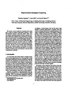
(a) Z (1)
(b) Θ(1) (27.60%)
(c) Z (3)
(d) Θ(3) (6.77%)
Figure 1. Visualization of matrices Z (t) and Θ(t) in the first and the third iterations of S3 C algorithm. Note that the first iteration of S3 C is effectively a SSC and hence the images of Z (1) and Θ(1) in panel (a) and (b) are the representation matrix and the structure matrix of SSC, in which Θ(1) is computed using the current clustering result. The structure matrix Θ(t) is used to reweight the computing of the representation matrix Z (t+1) in the next iteration. The images in panel (c) and (d) are the representation matrix Z (t) and structure matrix Θ(t) of S3 C when converged (t = 3). The percentage numbers in bracket are the corresponding clustering errors. For ease of visualization, we computed the entry-wise absolute value and amplified each entry |Zij | and Θij by a factor of 500.
can be expressed as a linear combination of other data points as X = XZ with diag(Z) = 0, where Z ∈ IRN ×N is a matrix of coefficients whose (i, j) entry |Zij | captures the similarity between points i and j. The matrix of coefficients is called subspace structured provided that Zij ̸= 0 only if points i and j lie in the same subspace. In existing approaches [10, 25, 28], one exploits the selfexpressiveness property by adding some penalty term on Z, e.g., ℓ1 [9, 10], ∥ · ∥∗ [25, 24], ∥ · ∥F [28], or even a data dependent norm [27]. However, these approaches do not exploit the fact that the representation matrix Z and the segmentation matrix Q both try to capture the segmentation of the data. Indeed, recall that the approach in (1) computes the segmentation Q by applying spectral clustering to the similarity matrix |Z| + |Z ⊤ |. For the time being, imagine that the exact segmentation matrix Q was known. In order to capture the fact that the zero patterns of Z and Q are related, observe that when Zij ̸= 0 points i and j are in the same subspace, hence we must have q(i) = q(j) , where q(i) and q(j) are the i-th and j-th row of matrix Q, respectively. Therefore, we can quantify the disagreement between Z and Q by using the following subspace structured measure of Z: ∥Θ ⊙ Z∥0 =
∑ i,j:q(i) ̸=q(j)
I{|Zij |̸=0}
(3)
where Θij = 12 ∥q(i) − q(j) ∥2 , the operator ⊙ indicates the Hadamard product (i.e., element-wise product) and I is an indicator function. Since Θij ∈ {0, 1}, the cost in (3) effectively counts the number of nonzero entries in Z when data point i and j are in different subspaces. Unfortunately the subspace structured measure of Z is combinatorial in nature and hence leads to an NP-hard problem. Instead, we propose a relaxed counterpart, called the subspace structured norm of Z with respect to (w.r.t.) Q,
denoted as ∥Z∥Q , which is defined as follows: 1 . ∑ ∥Z∥Q = |Zij |( ∥q(i) − q(j) ∥2 ) = ∥Θ ⊙ Z∥1 . 2 i,j
(4)
Note that when the subspace detection property [37] holds, i.e., Zij = 0 whenever points i and j lie in different subspace, then the subspace structured norm ∥Z∥Q vanishes; otherwise, it is positive. In practice, of course, the true segmentation matrix Q is unknown. Nevertheless, ∥Z∥Q still provides a useful measure of the agreement between the segmentation matrix Q and the representation matrix Z. Therefore, a straightforward approach to subspace clustering is to use the subspace structured norm ∥Z∥Q directly to replace the first term ∥Z∥κ in problem (1) and optimize over Z, E, and Q simultaneously. By doing so, we have a unified optimization framework, which ensures consistency between the representation coefficients and the subspace segmentation by solving the following optimization problem: min ∥Z∥Q + λ∥E∥ℓ
Z,E,Q
s.t. X = XZ + E, diag(Z) = 0, Q ∈ Q.
(5)
The optimization problem in (5) can be solved by alternatively solving (Z, E) and Q. Given Q, the problem is a convex program for (Z, E) which can be solve efficiently using the alternating direction method of multipliers (ADMM) [4][23]. Given (Z, E), the solution for Q can be computed approximately by spectral clustering. To see this, note that the ∥Z∥Q can be rewritten as: ∑ 1 ∥Z∥Q = |Zij |( ∥q(i) − q(j) ∥2 ) 2 i,j =
1∑ Ai,j ∥q(i) − q(j) ∥22 2 i,j
¯ = trace(Q⊤ LQ),
(6)
where Aij = 12 (|Zij | + |Zji |) measures the similarity of ¯=D ¯ − A is a graph Laplacian, and D ¯ points i and j, L ∑ is a ¯ diagonal matrix whose diagonal entries are Djj = i Aij . Consequently, given Z, we can find Q by solving the problem: ¯ min trace(Q⊤ LQ) Q
s.t.
Q ∈ Q,
(7)
which is the problem solved approximately by spectral clustering by relaxing the constraint Q ∈ Q to Q⊤ Q = I. Although the formulation in (5) is appealing since it formulates the two separate stages in self-expression model based spectral clustering methods into a unified optimization framework, it suffers from two critical shortcomings: a) it depends strongly on initialization, and b) it depends tightly upon solving the subspace segmentation matrix Q which is combinatorial problem. Note that: • When Q is initialized arbitrarily as a segmentation matrix in Q, the iterations of the optimization problem will be “trapped” within the initialized support of Θ which is defined by the initial Q. • If Q is initialized from an infeasible solution, which corresponds to treating each single data point as one subspace, then the first iteration for solving Z is equivalent to a standard SSC.1 Unfortunately, after solving one iteration of the problem, we then return to the previous issue, where we become trapped within the first estimated clustering. To remedy the drawbacks of the unified optimization framework mentioned above, we need to incorporate additional structure into the subspace structured norm ∥Z∥Q .
2.2. Structured Sparse Subspace Clustering (S3 C) Recall that in existing work, the ℓ1 norm ∥Z∥1 used in SSC, the nuclear norm ∥Z∥∗ used in LRR, the Frobenius norm ∥Z∥F used in LSR, or the TraceLasso norm used in CASS are all powerful means to detect subspaces. While any of them could potentially be incorporated into the subspace structured norm, here we adopt the ℓ1 norm and define a subspace structured ℓ1 norm of Z as follows: . ∥Z∥1,Q = ∥Z∥1 + α∥Θ ⊙ Z∥1 = ∥(11⊤ + αΘ) ⊙ Z∥1 ∑ α = |Zij |(1 + ∥q(i) − q(j) ∥2 ), 2 i,j
(8)
where α > 0 is a tradeoff parameter. Clearly, the first term is the standard ℓ1 norm used in SSC. Therefore the subspace structured ℓ1 norm can be viewed as an ℓ1 norm augmented 1 In this case, since Θ = 11⊤ − diag(1), we have ∥Z∥ Q = ∥Z∥1 − diag(Z).
by an extra penalty on Zij when points i and j are in different subspaces according to the segmentation matrix Q. The reasons we prefer to use the ℓ1 norm are two fold: • Since both the ℓ1 norm and the subspace structured norm (w.r.t. Q) are based on the ℓ1 norm, this leads to a combined norm that also has the structure of the ℓ1 norm. We will see later that this will facilitate updating the coefficients of Z. • The second reason to use the ℓ1 norm is the great theoretical guarantees for correctness enjoyed by SSC, which is applicable to detect subspace even when subspaces are overlapping [37]. Equipped with the subspace structured ℓ1 norm of Z, we can reformulate the unified optimization framework in (5) for subspace clustering as follows: min ∥Z∥1,Q + λ∥E∥ℓ
Z,E,Q
s.t. X = XZ + E, diag(Z) = 0, Q ∈ Q.
(9)
where the norm ∥ · ∥ℓ on the error term E depends upon the prior knowledge about the pattern of noise or corruptions.2 We call problem (9) Structured Sparse Subspace Clustering (SSSC or S3 C). Discussions. Notice that the S3 C framework in (9) generalizes SSC because, instead of first solving for a sparse representation to find Z and then applying spectral clustering to the affinity |Z| + |Z ⊤ | to obtain the segmentation, in (9) we simultaneously search for the sparse representation Z and the segmentation Q. Our S3 C differs from the reweighted ℓ1 minimization [6] in that what we use to reweight is not Z itself but rather a subspace structure matrix Θ. Compared to [13], which adds an extra block-diagonal constraint into the expressiveness model, whereas our framework encourages consistency between the representation matrix and the estimated segmentation matrix. It should also be noted that our subspace structured norm can be used in conjunction with other self-expressiveness based methods [25][28][27], and can also be combined with other weighted methods [35] or methods with extra regularization [20].
3. An Alternating Minimization Algorithm for Structured Sparse Subspace Clustering In this section, we propose a solution to the optimization problem in (9) based on solving the following two subproblems alternatively: 2 For example, the Frobenius norm will be used if the data are contaminated with dense noise; the ℓ1 norm will be used if the data are contaminated with sparse corruptions; the ℓ2,1 norm will be used if the data are contaminated with gross corruptions over a few columns; or the combination of these norms will be used for mixed patterns of noise and corruptions.
Algorithm 1 (ADMM for solving problem (11)) Input: Data matrix X, Θ0 , λ, and α. Initialize: Θ = Θ0 , E = 0, C = Z = Z0 , Y (1) = 0, Y (2) = 0, ϵ = 10−6 , ρ = 1.1 while not converged do Update Zt , Ct , and Et ; (1) (2) Update Yt and Yt ; Update µt+1 ← ρµt ; Check the convergence condition ∥X − XC − E∥∞ < ϵ; if not converged, then set t ← t + 1. end while Output: Zt+1 and Et+1
1. Find Z and E given Q by solving a weighted sparse representation problem.
3.1. Subspace Structured Sparse Representation Given the segmentation matrix Q (or the structure matrix Θ), we solve for Z and E by solving the following structured sparse representation problem min ∥Z∥1,Q + λ∥E∥ℓ (10)
s.t. X = XZ + E, diag(Z) = 0,
Z,C,E
ij Z˜t+1 = S µ1
t
L(Z, C, E, Y
,Y
(1)
C
(2) (16) +⟨Yt , C − Zt + diag(Zt )⟩ µt + (∥X −XC −Et ∥2F + ∥C −Zt +diag(Zt )∥2F ), 2
whose solution is given by
+Zt −diag(Zt )−
Et+1 = arg min
)
+⟨Y , C − Z + diag(Z)⟩ µ + (∥X − XC − E∥2F + ∥C − Z + diag(Z)∥2F ), 2
(12)
where Y (1) and Y (2) are matrices of Lagrange multipliers, and µ > 0 is a parameter. To find a saddle point for L, we update each of Z, C, E, Y (1) , and Y (2) alternatively while keeping the other variables are fixed. Update for Z. We update Z by solving the following problem: 1 1 Zt+1 = arg min ∥Z∥1,Q + ∥Z − diag(Z) − Ut ∥2F , (13) µt 2 Z
1 (1) Y ) µt t
1 (2) Y ]. µt t
(17)
Update for E. While other variables are fixed, we update E as follows:
E
=∥Z∥1,Q + λ∥E∥ℓ + ⟨Y (1) , X − XC − E⟩ (2)
(15)
Ct+1 = arg min⟨Yt , X − XC − Et ⟩
(11)
We solve this problem using the Alternating Direction Method of Multipliers (ADMM) [23],[4]. The augmented Lagrangian is given by: (2)
ij (1+αΘij ) (Ut ).
where Sτ (·) is the shrinkage thresholding operator. Note that the subspace structured ℓ1 norm causes a minor change to the algorithm used to compute Z from the standard SSC – because of the homogeneity in the two terms. Namely, rather than soft-thresholding all the entries of matrix Ut with a constant value, we threshold the entries of matrix Ut with different values that depend on Θij .
s.t. X = XC + E, C = Z − diag(Z).
(1)
(14)
where the (i, j) entry of Z˜ is given by
Ct+1 = (X ⊤ X +I)−1 [X ⊤ (X −Et −
which is equivalent to the following problem min ∥Z∥1,Q + λ∥E∥ℓ
Zt+1 = Z˜t+1 − diag(Z˜t+1 ),
Update for C. We update C by solving the following problem:
2. Find Q given Z and E by spectral clustering.
Z,E
(2)
where ∥Z∥1,Q = ∥Z∥1 +α∥Θ⊙Z∥1 and Ut = Ct + µ1t Yt . The closed-form solution for Z is given as
λ 1 ∥E∥ℓ + ∥E − Vt ∥2F µt 2
where Vt = X − XCt+1 + for E, then
(1) 1 µt Yt .
(18)
If we use the ℓ1 norm
Et+1 = S λ (Vt ). µt
(19)
Update for Y (1) and Y (2) . The update for the Lagrange multipliers is a simple gradient ascent step Yt+1 = Yt
(1)
(1)
+ µt (X − XCt+1 − Et+1 ),
(2) Yt+1
(2) Yt
+ µt (Ct+1 − Zt+1 + diag(Zt+1 )).
=
(20)
For clarity, we summarize the ADMM algorithm for solving problem (11) in Algorithm 1. For the details of the derivation, we refer the readers to [23, 4].
Algorithm 2 (S3 C) Input: Data matrix X and the number of subspaces k Initialize: Θ = 0, λ, α while not converged do Given Q, solve problem (10) via Alg. 1 to obtain (Z, E); Given (Z, E), solve problem (21) via spectral clustering to obtain Q; end while Output: Segmentation matrix Q
3.2. Spectral Clustering Given Z and E, problem (9) reduces to the following problem: min ∥Z∥1,Q s.t. Q ∈ Q.
(21)
Q
Recall that ∥Z∥1,Q = ∥Z∥1 + α∥Θ ⊙ Z∥1 and observe that the first term in ∥Z∥1,Q is not a function of Q, hence it can be dropped. Consequently problem (21) reduces to problem (7), which can be approximately solved with spectral clustering [44]. More specifically, by relaxing the constraint that Q ∈ Q to requiring that Q be an orthogonal matrix, i.e., Q⊤ Q = I, we obtain: min
Q∈IRN ×k
⊤¯
α trace(Q LQ)
s.t.
⊤
Q Q = I.
(22)
The solution to this relaxed problem can be found efficiently by eigenvalue decomposition. In particular, the columns of ¯ associated with the Q are given by the eigenvectors of L smallest k eigenvalues. The rows of Q are then used as input to the k-means algorithm, which produces a clustering of the rows of Q that can be used to produce a binary matrix Q ∈ {0, 1}N ×k such that Q1 = 1.
3.3. Algorithm Summary For clarity, we summarize the whole scheme to solving problem (9) in Algorithm 2. The algorithm alternates between solving for the matrices of sparse coefficients and the error (Z, E) given the segmentation Q using Algorithm 1 and solving for Q given (Z, E) using spectral clustering. While the problem solved by Algorithm 1 is a convex problem, there is no guarantee that the Algorithm 2 will converge to a global or local optimum because the solution for Q given (Z, E) is obtained in an approximate manner by relaxing the objective function. Nonetheless, our experiments show that the algorithm does converge in practice for appropriate settings of the parameters. Stopping Criterion. We terminate Algorithm 2 by checking the following condition ∥ΘT +1 − ΘT ∥∞ < 1,
(23)
(a)
(b)
Figure 2. Experimental Results on Synthetic Data Set. (a): The clustering errors as a function of α. (b): The histogram of numbers of iterations where α = 0.1 and Tmax = 10.
where T = 1, 2, . . . is the iteration index. Parameter Setting. In S3 C the parameters λ and α need to be set properly as in SSC [10]. Nevertheless, we observed that rather than using a fixed α to balance the two terms in the subspace structured ℓ1 norm ∥Z∥1,Q , the convergence could be improved by, e.g., using α ← να or using ν 1−T ∥Z∥1 +αν T −1 ∥Z∥Q in Algorithm 2, where ν > 1 and T = 1, 2, . . . is the iteration index.
4. Experiments In this section, we evaluate the proposed S3 C approach on a synthetic data set, a motion segmentation data set, and a face clustering data set to validate its effectiveness. Experimental Setup. Since that our S3 C is a generalization of the standard SSC [10], we keep all settings in S3 C the same as in SSC and thus the first iteration of S3 C is equivalent to a standard SSC. The S3 C specific parameters are set using ν 1−T ∥Z∥1 + αν T −1 ∥Z∥Q where α = 0.1, ν = 1.2, and Tmax = 10 by default. The λ and the ADMM parameters are kept the same for both S3 C and SSC. For each set of experiments, the average and median of subspace clustering error are recorded. The error (ERR) of subspace clustering is calculated by ˆ ) = 1 − max ERR(a, a π
N 1 ∑ 1{π(a)=ˆa} N i=1
(24)
ˆ ∈ {1, · · · , k}N are the original and estimated where a, a assignments of the columns in X to the k subspaces, and the maximum is with respect to all permutations π : {1, · · · , k}N → {1, · · · , k}N .
(25)
For the motion segmentation problem, we consider the Hopkins 155 database [39], which consists of 155 video sequences with 2 or 3 motions in each video corresponding to 2 or 3 low-dimensional subspaces. For the face clustering problem, we consider the Extended Yale B data set [14],
Corruptions (%)
80 %
90%
SSC 1.43 1.93 2.17 4.27 16.87 32.50 54.47 62.43 68.87 Our S3 C 0.30 0.33 0.90 2.97 10.70 23.67 50.50 60.70 67.97 Table 1. Clustering Errors on Synthetic Data Set. The best results are in bold font.
0
10%
20%
30%
40%
50 %
60%
70%
73.77 73.33
which consists of face images of 38 subjects, where the face images of each subject correspond to a low-dimensional subspace.
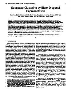
4.1. Experiments on Synthetic Data Figure 3. Example frames from videos in the Hopkins 155 [39].
Data Preparing. We construct k linear subspaces {Sj }kj=1 ⊂ IRn whose bases {Uj }kj=1 are the left singular matrixes computed from a random matrix Rj ∈ IRn×n . We sample Nj data points from each subspace j = 1, . . . , k as Xj = Uj Yj , where the entries of Yj ∈ IRd×Nj are i.i.d. samples from a standard Gaussian. Note that by doing so, the k linear subspaces are not necessarily orthogonal to each other. We then corrupt a certain percentage p = 10 − 90% of entries uniformly at random, e.g., for a column x chosen to corrupt, its observed vector is added by Gaussian noise with zero mean and variance 0.3∥x∥. We repeat each experiment for 20 trials. In our experiments, we set n = 100, d = 5, Nj = 10, and k = 15. Experimental results are presented in Table 1. Notice that our S3 C algorithm consistently outperforms SSC. To gain more insights into the sensitivity of S3 C to the parameter α, in Fig. 2 (a) we show the results of varying α over [0, 1] while holding the corruption level fixed at 55%. As could be observed that, our method works well for α ∈ [0.03, 0.30]. In Fig. 2 (b), we show the histogram of the numbers of iterations for S3 C to converge with α = 0.1 and Tmax = 10. As could be observed that, our S3 C converges in 2 ∼ 6 iterations on average. For the average time cost, SSC takes 1.46 seconds whereas our S3 C takes 8.05 seconds which is roughly 5.5 times of SSC’s on the synthetic data sets.
4.2. Data Visualization To show the effect of the subspace structured ℓ1 norm in S3 C intuitively, we take a subset of images of three subjects from the Extended Yale B data set, perform S3 C, and then visualize the representation matrix Z (t) and the subspace structure matrix Θ(t) , which are taken in the t-th iteration in S3 C. Note that the first iteration of S3 C is effectively a SSC since we use the same parameters. The visualization results are displayed in Fig. 1. We observe from Fig. 1 (a) that the structured sparse representation matrix Z (1) – which is effectively the sparse representation matrix of SSC – is not a clearly block-diagonal and leads to a degenerated clustering result as shown by the subspace structure matrix Θ(1) in Fig. 1 (b). In the third iteration (t = 3), S3 C yields a much better representation matrix Z (3) , as shown in Fig. 1 (c), and hence produces
a significantly improved clustering result as shown by the subspace structure matrix Θ(3) in Fig. 1 (d). While S3 C in this case did not yield a perfect block-diagonal representation matrix, the improvements still reduce the clustering error significantly – 27.60% vs. 6.77%.
4.3. Experiments on Hopkins 155 Database Motion segmentation refers to the problem of segmenting a video sequence with multiple rigidly moving objects into multiple spatiotemporal regions that correspond to the different motions in the scene (see Fig. 3). This problem is often solved by first extracting and tracking the spatial positions of a set of N feature points xf i ∈ IR2 through each frame f = 1, . . . , F of the video, and then clustering these feature points according to each one of the motions. Under the affine projection model, a feature point trajectory is formed by stacking the feature points xf i in the video as . ⊤ ⊤ 2F ⊤ . Since the trajectories asyi = [x⊤ 1i , x2i , · · · , xF i ] ∈ IR sociated with a single rigid motion lie in an affine subspace of IR2F of dimension at most 4 [38], the trajectories of k rigid motions lie in a union of k low-dimensional subspaces of IR2F . Therefore, the multi-view affine motion segmentation problem reduces to the subspace clustering problem. We compare our S3 C algorithm with SSC [10], LSA [46], LRR [25], LSR [28], BDSSC [13] and BDLRR [13] on the Hopkins 155 motion segmentation data set [39] for the multi-view affine motion segmentation without other postprocessing. Experimental results are presented in Table 2. Note that from the results in Table 2, the S3 C is again the best performing method; however, due to the fact that the Hopkins 155 database has a relatively low noise level, the improvement in performance over SSC is relatively minor.
4.4. Experiments on Extended Yale B Data Set The Extended Yale Database B [14] contains 2,414 frontal face images of 38 subjects, with approximately 64 frontal face images per subject taken under different illumination conditions. Given the face images of multiple subjects acquired under a fixed pose and varying illumination, we consider the problem of clustering the images according
Methods 2 motions ERR(%) 3 motions ERR(%) Total ERR(%)
Ave. Med. Ave. Med. Ave. Med.
LSA
LRR
BDLRR
LSR1
LSR2
BDSSC
SSC
Our S3 C
3.62 0.51 7.67 1.27 4.53 0.63
3.76 0.00 9.92 1.42 5.15 0.00
3.70 0.00 6.49 1.20 4.33 0.00
2.20 0.00 7.13 2.40 3.31 0.22
2.22 0.00 7.18 2.40 3.34 0.23
2.29 0.00 4.95 0.91 2.89 0.00
1.95 0.00 4.94 0.89 2.63 0.00
1.94 0.00 4.92 0.89 2.61 0.00
Table 2. Motion Segmentation Errors on Hopkins 155 Database. The best results are in bold font. No. subjects ERR (%)
2 Average
Median
3 Average
Median
LRR 6.74 7.03 9.30 LSR1 6.72 7.03 9.25 LSR2 6.74 7.03 9.29 CASS 10.95 6.25 13.94 LRSC [42] 3.15 2.34 4.71 BDSSC [13] 3.90 17.70 BDLRR [13] 3.91 10.02 LatLRR 2.54 0.78 4.21 SSC 1.87 0.00 3.35 S3 C† 1.43 0.00 3.09 S3 C ‡ 1.40 0.00 3.08 S3 C 1.27 0.00 2.71 Table 3. Clustering Errors on Extended Yale B Data Set. use α ← να.
5 Average
Median
8 Average
9.90 13.94 14.38 9.90 13.87 14.22 9.90 13.91 14.38 7.81 21.25 18.91 4.17 13.06 8.44 27.50 12.97 2.60 6.90 5.63 0.78 4.32 2.81 0.52 4.08 2.19 0.52 3.83 1.88 0.52 3.41 1.25 The best results are in bold font.
to their subjects. It has been shown that, under the Lambertian assumption, the images of a subject with a fixed pose and varying illumination lie close to a linear subspace of dimension 9 [18]. Thus, the collection of face images of multiple subjects lie close to a union of 9-dimensional subspaces. It should be noted that the Extended Yale B dataset is more challenging for subspace segmentation than the Hopkins 155 database due to heavy corruptions in the data. We compare the clustering errors of our proposed S3 C algorithm with SSC [10], LRR [25], LatLRR [26], LRSC [42], and other recently proposed algorithms, including LSR [28], CASS [27], and BDSSC [13] and BDLRR [13]. In our experiments, we follow the protocol introduced in [10]: a) each image is down-sampled to be 48 × 42 pixels and then vectorized to a 2,016-dimensional data point; b) the 38 subjects are then divided into 4 groups – subjects 1-10, 11-20, 21-30, and 31-38. We perform experiments using all choices of n ∈ {2, 3, 5, 8, 10} subjects in each of the first three groups and use all choices of n ∈ {2, 3, 5, 8} from the last group. For S3 C, SSC, LatLRR, and LRSC, we use the 2,016-dimensional vectors as inputs. For LatLRR and LRSC, we cite the results reported in [10] and [42], respectively. For LRR, LSR, and CASS, we use the procedure reported in [28]: use standard PCA to reduce the 2,016-dimensional data to 6k-dimensional data for k ∈ {2, 3, 5, 8, 10}. For BDSSC, and BDLRR, we directly cite the best results in their papers, which are based
Median
10 Average
Median
25.61 24.80 29.53 30.00 25.98 25.10 28.33 30.00 25.52 24.80 30.73 33.59 29.58 29.20 32.08 35.31 26.83 28.71 35.89 34.84 33.20 39.53 27.70 30.84 14.34 10.06 22.92 23.59 5.99 4.49 7.29 5.47 4.84 4.10 6.09 5.16 4.45 3.52 5.42 4.53 4.15 2.93 5.16 4.22 In S3 C† we fix α as 0.1 whereas in S3 C‡ we
on 9k-dimensional data. The full experimental results are presented in Table 3. Again, we observe that S3 C yields the lowest clustering errors across all experimental conditions.
5. Conclusion We described a unified optimization framework for the problem of subspace clustering. Moreover by introducing a subspace structured ℓ1 norm, we formulated the sparse subspace clustering algorithm into a unified optimization framework, termed as Structured Sparse Subspace Clustering (S3 C), in which the separate two stages of computing the sparse representation and applying the spectral clustering were elegantly merged together. We solved this problem efficiently via a combination of an alternating direction method of multipliers with spectral clustering. Experiments on a synthetic data set, the Hopkins 155 motion segmentation database, and the Extended Yale B data set demonstrated the effectiveness of our method.
Acknowledgment C.-G. Li was partially supported by National Natural Science Foundation of China under Grant Nos. 61175011 and 61273217, and Scientific Research Foundation for the Returned Overseas Chinese Scholars, Ministry of Education of China. R. Vidal was supported by the National Science Foundation under Grant No. 1447822.
References [1] P. Agarwal and N. Mustafa. k-means projective clustering. In ACM Symposium on Principles of database systems, 2004. 1 [2] C. Archambeau, N. Delannay, and M. Verleysen. Mixtures of robust probabilistic principal component analyzers. Neurocomputing, 71(7–9):1274–1282, 2008. 1 [3] T. Boult and L. Brown. Factorization-based segmentation of motions. In IEEE Workshop on Motion Understanding, pages 179–186, 1991. 1 [4] S. Boyd, N. Parikh, E. Chu, B. Peleato, and J. Eckstein. Distributed optimization and statistical learning via the alternating direction method of multipliers. Foundations and Trends in Machine Learning, 3(1):1–122, 2010. 3, 5 [5] P. S. Bradley and O. L. Mangasarian. k-plane clustering. Journal of Global Optimization, 16(1):23–32, 2000. 1 [6] E. Cand`es, M. Wakin, and S. Boyd. Enhancing sparsity by reweighted ℓ1 minimization. Journal of Fourier Analysis and Applications, 14(5):877–905, 2008. 4 [7] G. Chen and G. Lerman. Spectral curvature clustering (SCC). International Journal of Computer Vision, 81(3):317– 330, 2009. 1 [8] J. Costeira and T. Kanade. A multibody factorization method for independently moving objects. International Journal of Computer Vision, 29(3):159–179, 1998. 1 [9] E. Elhamifar and R. Vidal. Sparse subspace clustering. In IEEE Conference on Computer Vision and Pattern Recognition, 2009. 1, 3 [10] E. Elhamifar and R. Vidal. Sparse subspace clustering: Algorithm, theory, and applications. IEEE Transactions on Pattern Analysis and Machine Intelligence, 35(11):2765–2781, 2013. 1, 3, 6, 7, 8 [11] Z. Fan, J. Zhou, and Y. Wu. Multibody grouping by inference of multiple subspaces from high-dimensional data using oriented-frames. IEEE Transactions on Pattern Analysis and Machine Intelligence, 28(1):91–105, 2006. 1 [12] P. Favaro, R. Vidal, and A. Ravichandran. A closed form solution to robust subspace estimation and clustering. In IEEE Conference on Computer Vision and Pattern Recognition, 2011. 1 [13] J. Feng, Z. Lin, H. Xu, and S. Yan. Robust subspace segmentation with block-diagonal prior. In CVPR, 2014. 2, 4, 7, 8 [14] A. Georghiades, P. Belhumeur, and D. Kriegman. From few to many: Illumination cone models for face recognition under variable lighting and pose. IEEE Transactions on Pattern Analysis and Machine Intelligence, 23(6):643–660, 2001. 6, 7 [15] A. Goh and R. Vidal. Segmenting motions of different types by unsupervised manifold clustering. In IEEE Conference on Computer Vision and Pattern Recognition, 2007. 1 [16] E. Grave, G. Obozinski, and F. Bach. Trace lasso: a trace norm regularization for correlated designs. In NIPS, 2011. 2 [17] A. Gruber and Y. Weiss. Multibody factorization with uncertainty and missing data using the em algorithm. In IEEE Conference on Computer Vision and Pattern Recognition, volume I, pages 707–714, 2004. 1
[18] J. Ho, M. H. Yang, J. Lim, K. Lee, and D. Kriegman. Clustering appearances of objects under varying illumination conditions. In IEEE Conference on Computer Vision and Pattern Recognition, 2003. 1, 8 [19] W. Hong, J. Wright, K. Huang, and Y. Ma. Multi-scale hybrid linear models for lossy image representation. IEEE Trans. on Image Processing, 15(12):3655–3671, 2006. 1 [20] H. Hu, Z. Lin, J. Feng, and J. Zhou. Smooth representation clustering. In CVPR, 2014. 2, 4 [21] K. Huang, Y. Ma, and R. Vidal. Minimum effective dimension for mixtures of subspaces: A robust GPCA algorithm and its applications. In IEEE Conference on Computer Vision and Pattern Recognition, volume II, pages 631–638, 2004. 1 [22] A. Leonardis, H. Bischof, and J. Maver. Multiple eigenspaces. Pattern Recognition, 35(11):2613–2627, 2002. 1 [23] Z. Lin, M. Chen, L. Wu, and Y. Ma. The augmented Lagrange multiplier method for exact recovery of corrupted low-rank matrices. arXiv:1009.5055v2, 2011. 3, 5 [24] G. Liu, Z. Lin, S. Yan, J. Sun, and Y. Ma. Robust recovery of subspace structures by low-rank representation. IEEE Trans. Pattern Analysis and Machine Intelligence, 35(1):171–184, Jan 2013. 1, 3 [25] G. Liu, Z. Lin, and Y. Yu. Robust subspace segmentation by low-rank representation. In International Conference on Machine Learning, 2010. 1, 3, 4, 7, 8 [26] G. Liu and S. Yan. Latent low-rank representation for subspace segmentation and feature extraction. International Conference on Computer Vision, 2011. 2, 8 [27] C. Lu, Z. Lin, and S. Yan. Correlation adaptive subspace segmentation by trace lasso. In ICCV, 2013. 1, 2, 3, 4, 8 [28] C. Lu, H. Min, Z.-Q. Zhao, L. Zhu, D.-S. Huang, and S. Yan. Robust and efficient subspace segmentation via least squares regression. In Proceedings of European Conference on Computer Vision, 2012. 1, 2, 3, 4, 7, 8 [29] C. Lu, S. Yan, and Z. Lin. Correntropy induced l2 graph for robust subspace clustering. In ICCV, 2013. 1, 2 [30] D. Luo, F. Nie, C. H. Q. Ding, and H. Huang. Multi-subspace representation and discovery. In ECML/PKDD, pages 405– 420, 2011. 2 [31] Y. Ma, H. Derksen, W. Hong, and J. Wright. Segmentation of multivariate mixed data via lossy coding and compression. IEEE Transactions on Pattern Analysis and Machine Intelligence, 29(9):1546–1562, 2007. 1 [32] Y. Ma, A. Y. Yang, H. Derksen, and R. Fossum. Estimation of subspace arrangements with applications in modeling and segmenting mixed data. SIAM Review, 50(3):413–458, 2008. 1 [33] V. M. Patel, H. V. Nguyen, and R. Vidal. Latent space sparse subspace clustering. In IEEE International Conference on Computer Vision, 2013. 2 [34] V. M. Patel and R. Vidal. Kernel sparse subspace clustering. In International Conference on Image Processing, 2014. 2 [35] D. Pham, S. Budhaditya, D. Phung, and S. Venkatesh. Improved subspace clustering via exploitation of spatial constraints. In CVPR, 2012. 2, 4
[36] S. Rao, R. Tron, R. Vidal, and Y. Ma. Motion segmentation in the presence of outlying, incomplete, or corrupted trajectories. IEEE Transactions on Pattern Analysis and Machine Intelligence, 32(10):1832–1845, 2010. 1 [37] M. Soltanolkotabi and E. J. Cand`es. A geometric analysis of subspace clustering with outliers. Annals of Statistics, 40(4):2195–2238, 2012. 3, 4 [38] C. Tomasi and T. Kanade. Shape and motion from image streams under orthography. International Journal of Computer Vision, 9(2):137–154, 1992. 1, 7 [39] R. Tron and R. Vidal. A benchmark for the comparison of 3-D motion segmentation algorithms. In IEEE Conference on Computer Vision and Pattern Recognition, 2007. 6, 7 [40] P. Tseng. Nearest q-flat to m points. Journal of Optimization Theory and Applications, 105(1):249–252, 2000. 1 [41] R. Vidal. Subspace clustering. IEEE Signal Processing Magazine, 28(3):52–68, March 2011. 1 [42] R. Vidal and P. Favaro. Low rank subspace clustering (LRSC). Pattern Recognition Letters, 43:47–61, 2014. 1, 8 [43] R. Vidal, Y. Ma, and S. Sastry. Generalized Principal Component Analysis (GPCA). IEEE Transactions on Pattern Analysis and Machine Intelligence, 27(12):1–15, 2005. 1 [44] U. von Luxburg. A tutorial on spectral clustering. Statistics and Computing, 17, 2007. 6 [45] S. Wang, X. Yuan, T. Yao, S. Yan, and J. Shen. Efficient subspace segmentation via quadratic programming. In AAAI, 2011. 2 [46] J. Yan and M. Pollefeys. A general framework for motion segmentation: Independent, articulated, rigid, non-rigid, degenerate and non-degenerate. In European Conference on Computer Vision, pages 94–106, 2006. 1, 7 [47] A. Y. Yang, S. Rao, and Y. Ma. Robust statistical estimation and segmentation of multiple subspaces. In Workshop on 25 years of RANSAC, 2006. 1 [48] T. Zhang, A. Szlam, and G. Lerman. Median k-flats for hybrid linear modeling with many outliers. In Workshop on Subspace Methods, 2009. 1 [49] T. Zhang, A. Szlam, Y. Wang, and G. Lerman. Hybrid linear modeling via local best-fit flats. International Journal of Computer Vision, 100(3):217–240, 2012. 1