56
Int. J. Logistics Economics and Globalisation, Vol. 6, No. 1, 2014
Non-iterative algorithm for finding shortest route Daniel Maposa* Monash South Africa Campus, Monash University Australia, Private Bag X60, Roodepoort, 1725, South Africa E-mail:
[email protected] *Corresponding author
Ndava Constantine Mupondo and Trust Tawanda Department of Applied Mathematics, National University of Science and Technology, P.O. Box AC 939, Ascot, Bulawayo, Zimbabwe E-mail:
[email protected] E-mail:
[email protected] Abstract: The use of non-iterative shortest route algorithm for finding shortest route between points in a network is illustrated. The non-iterative approach can be applied to various network problems that can be solved using shortest route algorithm and provides a solution with much less effort. The algorithm makes use of an n × n tableau to produce an optimum solution. The non-iterative technique provides an efficient solution procedure in terms of computational savings for large versions of network problems. The study revealed that problems can be solved using a reasonable amount of computer time by the non-iterative algorithm when other approaches are computationally unrealistic. This paper also establishes that the travelling salesman problem can be solved by non-iterative approach. Keywords: travelling salesman; algorithm; non-iterative; shortest route; tableau. Reference to this paper should be made as follows: Maposa, D., Mupondo, N.C. and Tawanda, T. (2014) ‘Non-iterative algorithm for finding shortest route’, Int. J. Logistics Economics and Globalisation, Vol. 6, No. 1, pp.56–77. Biographical notes: Daniel Maposa is a Lecturer of Business Statistics and Business Data Modelling at Monash University (South Africa campus). He holds an honours degree in Applied Mathematics and a Master of Science degree in Operations Research and Statistics. He is currently doing a PhD in Statistics of Extremes with applications to floods on part-time basis with University of Limpopo, South Africa. He has also taught several statistics courses and applied mathematics courses at University of Limpopo, South Africa and National University of Science and Technology (NUST), Zimbabwe.
Copyright © 2014 Inderscience Enterprises Ltd.
Non-iterative algorithm for finding shortest route
57
Ndava Constantine Mupondo is a Lecturer of Operations Research courses at National University of Science and Technology (NUST), Zimbabwe. He holds an honours degree and a Master of Science degree in Operations Research from the same university. Trust Tawanda holds an Honours degree in Operations Research and Statistics from the National University of Science and Technology (NUST), Zimbabwe. He is currently doing his Masters of Philosophy in Operations Research and Statistics from the same university, specialising in combinatorial optimisation and graph networks. This paper is a revised and expanded version of a paper entitled ‘Non-iterative algorithm for finding shortest route’ presented at the Operations Research Society of South Africa (ORSSA 2011) Conference, Victoria Falls, Zimbabwe, 16–19 September 2011.
1
Introduction
Many practical real-world problems can be formulated in a network, for example, the planning of networks, communication systems and large scale projects are common applications of network models (Markland and Sweigart, 1987; Ji et al., 2007; Lee and Wong, 2010; Hao-Yu et al., 2011). Solutions to such problems, using network models, can be very effectively conveyed to managers. There are a number of transportation applications that require the use of heuristic shortest route algorithms, so as to reduce distance and time taken to calculate the optimum route. The shortest route algorithms help minimise travel distance in a given network (Winston, 2004). They determine the shortest path between any two given nodes in a network as well as finding the optimal route from the source to sink (Hillier and Lieberman, 2001). In this paper we present a non-iterative algorithm for finding the shortest route.
1.1 The shortest route problem The shortest route problem is concerned with finding the shortest paths from an origin to a destination through a connected network, given the distances associated with the respective branches of the network (Winston, 2004). Shortest time problems are often of equal interest to shortest route problems and such problems arise frequently in connection with transportation networks, delivery and communication networks (Ahuja et al., 1993; Reader and Stair, 2004). Although the shortest route can be formulated and solved using linear programming, a simpler and relatively more efficient solution procedure has been developed in this study. This procedure is now presented and illustrated by means of an example.
1.2 Terminology and notation for network problems We define a network as a set of junction points called nodes or events that are connected by flow routes called branches or activities (or ‘arcs’, ‘links’, ‘connectors’, or ‘edges’) (Markland and Sweigart, 1987). In network, circles represent nodes and the lines connecting the circles are the branches.
58
D. Maposa et al.
According to Markland and Sweigart (1987) the nodes in a network typically represent physical locations, such as cities, airports, terminals and dumping stations. The branches typically represent connecting roads, air routes, pipelines or cables. The origin in a network is called the source node and the destination is called the sink node. A source node has an orientation such that all flow moves away from it and a sink node has an orientation such that all flow moves into it (Gallo and Pallottino, 1982, 1988; Hao-Yu et al., 2011). Section 2 gives a brief review of some common algorithms, Section 3 discusses the novel non-iterative algorithm with the aid of an example, while Section 4 discusses and Section 5 concludes the paper and finally the references list section.
2
Brief review of commonly used algorithms
In this section we review four common algorithms namely dynamic programming, simulated annealing, Dijkstra’s algorithm and Floyd’s algorithm.
2.1 Dynamic programming Dynamic programming is based on the idea of dividing the problem into stages. The outcome of the decision at one stage affects the decision and outcome at the next stage of the problem (Lee and Wong, 2010). Its use typically requires that a problem be broken down into a series of smaller sub-problems that are solved sequentially (Goldberg and Silverstein, 1997). The overall problem is decomposed into sub-problems called stages. The final stage (n) of the problem is analysed and solved for all of the possible conditions or states. Each preceding stage is solved, working backward from the final stage of the problem (Hillier and Lieberman, 2001). The problem is enlarged at each subsequent iteration by increasing the number of stages left by one to go to complete the journey. This involves making an optimal policy decision for the intermediate stage being linked to its preceding stage by a recursion relationship that involves a return function at each stage of the problem. The return at a particular stage is the net benefit that accrues at that stage due to the policy decision selected and its interaction with the state of the system. The stage of the problem is solved and when this has been accomplished the optimal solution has been obtained (Hillier and Lieberman, 2001).
2.2 Simulated annealing Simulated annealing is a technique that is used to find the shortest distance in a network. It makes use of the assumption that each node in the network is visited at most once and the source node is also the destination node in the network. Nodes in the network are swapped until the optimal route is obtained (Hillier and Lieberman, 2001; Winston, 2004).
2.3 Dijkstra’s algorithm The Dijkstra’s algorithm was discovered by a pioneering mathematician and programmer Dijkstra (1934–2002) (Dijkstra, 1959; Goldberg and Silverstein, 1997; Winston, 2004).
Non-iterative algorithm for finding shortest route
59
The algorithm finds the shortest path to all nodes from an original node. The algorithm expands outwards from the source node recursively considering every node that is closer in terms of shortest path distance until it reaches the destination (Dijkstra, 1959; Goldberg and Silverstein, 1997). When understood in this way it is clear how the algorithm necessarily finds the shortest route. However, it may reveal one of the algorithm’s weaknesses that it is relatively slow in some topologies (Fredman and Tarjan, 1987).
2.4 Floyd’s algorithm Floyd’s algorithm is more general than Dijkstra’s algorithm because it determines the shortest route between any two nodes in the network. The algorithm presents an n-node network as an n × n square matrix. Iterations are used to reach the optimal solution (Goldberg and Silverstein, 1997; Nguyen et al., 2002; Ji et al., 2007). In general all of the algorithms reviewed in this section (dynamic programming, simulated annealing, Dijkstra’s and Floyd’s algorithm) produce the optimal solutions using different procedures and reach the optimal solution after a number of iterations which consume a lot of resources and time. As the number of nodes in a network increases, the iterations increase respectively.
3
Non-iterative method
In an attempt to minimise time taken as well as number of iterations when solving shortest route problems, an alternative novel algorithm called non-iterative is proposed in this study. The proposed non-iterative algorithm captures aspects of shortest route problems, salesman’s problem etc. The algorithm makes use of an n × n tableau to produce an optimum solution. It can be applied in directed and non-directed networks. It can also be used to find the shortest route from source node to destination node in any given network. The non-iterative method is not well documented in literature and thus to the best of our knowledge it has not been previously published.
3.1 Assumptions The use of the non-iterative procedure assumes that: 1
the direct distance, dij, between any two nodes in the network of n nodes is given
2
all such distances are non-negative.
3.2 Methodology of the non-iterative shortest route technique The solution procedure proceeds in a fashion that identifies the optimal policy or solution. The fundamental stages in the non-iterative technique to shortest route are summarised in the next subsections.
60
D. Maposa et al.
3.3 Non-iterative tableau This is an n × n tableau where n is the number of nodes in a given network. All distances from one node to another node are entered in this tableau respectively. This tableau associates with an asterisk (*) to indicate that distance of a point to the same (i.e., itself) is zero. This asterisk has three meanings in the algorithm: 1
it shows a zero distance between any two given nodes
2
it reflects indirect link between two given nodes
3
it represents indirect routes or restricted routes.
3.4 Notations of the algorithm 1
Rn(i) representing row i, where i = 1, 2, 3... n
2
Cm(j) representing row j, where j = 1, 2, 3... m
3
Rn(i)c is equivalent to Cn(i)
4
Cn(i)r is equivalent to Rn(i).
3.5 Steps of the algorithm There are basically four steps involved in the non-iterative solution procedure. 1
create a distance tableau, with n rows and n columns and enter the corresponding distances, where n is the number of nodes in a given network
2
identify the smallest distance recorded in the first row and encircle it
3
consider the row that corresponds to the column where the smallest distance recorded lies, in the original row node and perform step 1
4
in the case where the column leads to a row that include the already encircled number, neglect the value and consider the next least value in that row
5
continue with steps 1 and 2 until all rows and columns are satisfied at most once.
NB •
The accepted smallest distance in a column has to be encircled.
•
In case that a row has at least two equal smallest distances, we use them separately to find respective solutions. Compare the respective solutions to find which one yields an optimal solution.
•
Each column and row has to be satisfied at most once. If it happens that the shortest distance lies in a column that has been satisfied then do not consider it, cancel it out and look for a second smallest distance recorded in that row that does not lie in a satisfied column.
Non-iterative algorithm for finding shortest route
61
3.6 An illustration of the non-iterative approach compared with other techniques Example 1 Using the Dijkstra’s algorithm and non-iterative technique. The network (Figure 1) gives the routes and their lengths in miles between city one (node 1) and four other cities (node 2 to 5). Determine the shortest route between city one and the other remaining four cities. Figure 1
Routes and their lengths in miles between cities 1 to 5
2
15 4
20 100
50
10
1
30
60 3
5
3.6.1 Solution by Dijkstra’s algorithm 3.6.1.1 Procedure The computations of the algorithm advance from node I to an immediately succeeding node j using a special labelling procedure. Let ui be the shortest distance from source node 1 to node I and define dij(≥ 0) as the length of arc (I, j). Then the label for node j is defined as
[u j , i ] = [ui + dij , i ] , dij ≥ 0 Node labels in Dijkstra’s algorithm are of two types: temporary and permanent. A temporary label can be replaced with another label if a shorter route to the same node can be found. At the point when it becomes evident that no better route can be found, the status of the temporary label is changed to permanent. The steps of the algorithm are summarised as follows. Step 0 Step i a
Label the source node (node 1) with a permanent label [0, –]. Set I = 1. Compute the temporary labels [ui + dij, i] for each node j that can be reached from node I, provided j is not permanently labelled. If node j is already labelled with [ui, k] through another node k and if ui + dij < uj, replace [uj, k] with [ui + dij, i].
62
D. Maposa et al. b
If all the nodes have been permanent labels, stop. Otherwise, select the label [ui, s] with the shortest distance (= ur) from among all the temporary labels (break ties arbitrarily). Set i = r and repeat step i.
3.6.1.2 Solution Iteration 0. Assign the permanent label [0, –] to node 1. Iteration 1. Nodes 2 and 3 can be reached from (the last permanently labelled) node 1. Thus, the list of labelled nodes (temporary and permanent) becomes: Node
Label
Status
1
[0, –]
Permanent
2
[0 + 100, 1] = [100, 1]
Temporary
3
[0 + 30, 1] = [30, 1]
Temporary
For the two temporary labels [100, 1] and [30, 1], node 3 yields the smaller distance (u3 = 30). Thus, the status of node 3 is changed to permanent. Iteration 2. Node 4 and 5 can be reached from node 3 and the list of labelled nodes becomes: Node
Label
Status
1
[0, –]
Permanent
2
[100, 1]
Temporary
3
[30, 1]
Permanent
4
[30 + 10, 3] = [40, 3]
Temporary
5
[30 + 60, 3] = [90, 3]
Temporary
The status of the temporary label [40, 3] at node 4 is changed to permanent (u4 = 40). Iteration 3. Nodes 2 and 5 can be reached from node 4. Thus, the list of labelled nodes is updated as Label
Status
1
Node
[0, –]
Permanent
2
[40 + 15, 4] =[55, 4]
Temporary
3
[30, 1]
Permanent
4
[40, 3]
Permanent
5
[90, 3] or [40 + 50, 4] = [90, 4]
Temporary
Node 2’s temporary label [100, 1] in iteration 2 is changed to [55, 4] in Iteration 3 to indicate that a shorter route has been found through node 4. Also, in Iteration 3, node 5 has two alternative labels with the same distance u5 = 90. The list of iteration 3 shows that node 2 must be permanently labelled. Iteration 4. Only node 3 can be reached from node 2. However, because node 3 is permanently labelled, it cannot be labelled. The new list of labels thus remains the same as in Iteration 3 except that the label at node 2 is permanent. This leaves node 5 as the
Non-iterative algorithm for finding shortest route
63
only temporary label. Because node 5 does not lead to other nodes, its status is converted to permanent and the process ends. Thus, the desired route is 1 – 3 – 4 – 2 with a total length of 55 miles.
3.6.2 Solution by non-iterative algorithm Step 1
Step 2
Construct the distance tableau and enter the respective distances 1
2
3
4
5
1
*
100
30
*
*
2
*
*
20
*
*
3
*
*
*
*
*
5
*
15 *
10 *
60
4
*
*
*
50
In this case the objective function is to find the shortest route between city one and the other four cities. Consider row node one Rn(1), the smallest distance recorded is 30 miles. This lies where Rn(1) intersects Cm(3). The next thing to consider the row corresponding to Cm(3) which is Rn(3). 10 is the smallest distance recorded in Rn(3), but our value lies where Rn(3) intersects Rm(4), by considering the corresponding row which is Rn(4). In this case the smallest distance recorded in this row is 15 and it lies where Rn(4) intersects Cm(2), considering the corresponding row of Cm(2) thus Rn(2), the smallest value is 20. Since our value lies in a satisfied column we consider it out and look for the second value in that row and in this case there is nothing hence we are done. The optimal solution is 1 – 3 – 4 – 2. The total length is 55 miles.
Example 2 Using the Floyd’s algorithm and non-iterative technique. For the network in Figure 2, find the shortest routes between every two nodes. The distance (in miles) is given on the arcs. Arc (3, 5) is directional so that no traffic is allowed from node 5 to node 3. All the other arcs traffic is in both directions. Figure 2
Network of routes between cities
2
4 5
3 4 6
1
5 10 3
15
64
D. Maposa et al.
3.6.3 Solution by Floyd’s algorithm 3.6.3.1 Procedure The algorithm represents an n-node network as a square matrix with n rows and n columns. Entry (I, j) of the matrix gives the distance dij from node I to node j, which is finite if it is linked directly to j and infinite otherwise. Given three nodes I, J and k with connecting distances, it is shorter to reach k from I passing through j if dij + d jk < dik
In this case, it is optimal to replace the direct route from I – k with the direct route I – j – k . This triple operation exchange is applied systematically to the network using the following steps: •
Step 0. Define the starting distance matrix D0 and node sequence matrix S0 as given subsequently. The diagonal elements are marked with (–) to indicates that they are blocked. Set k = 1.
•
General step k. Define row k and column k as pivot row and column. Apply the triple operation to each element dij in Dk–1, for all I and j. If the condition dik + d kj < dij , (i ≠ k , j ≠ k , i ≠ j )
Is satisfied, make the following changes: a
create Dk by replacing dij in Dk–1 with dik + dkj
b
create Sk by replacing sij in Sk–1 with k. Set k = k + 1 and repeat step k.
After n steps, we can determine the shortest route between nodes I and j from the matrices Dn and Sn using the following rules: 1
From Dn, dij gives the shortest distance between nodes i and j.
2
From Sn, determine the intermediate node k = sij, which yields the route I –k –j. If skj = k and sij = j, stop; all the intermediate nodes of the route have been found. Otherwise, repeat the procedure between nodes I and k and nodes k and j.
3.6.3.2 Solution Iteration 0. The matrices D0 and S0 give the initial representation of the network. D0 is symmetric except that d53 = ∞ because no traffic is allowed from node 5 to node 3. D0
S0
1
2
3
4
5
1
2
3
1
-
3
10
∞
∞
2
3
-
5
∞
3
10
6
4
∞
∞ 5
∞ 6
-
5
∞
∞
∞
4
4
5
1
-
2
3
4
5
2
1
-
4
5
15
3
1
4
5
4
4
1
2 2
3 3
-
5
-
5
1
2
3
4
-
Non-iterative algorithm for finding shortest route
65
Iteration 1. The pivot row and the pivot column are given by the (shaded) first row and first column (k = 1), as shown in the matrix D0. The double-boxed elements, d23 and d32 are the only ones that can be improved by the triple operation. Thus, to obtain D1 and S1 from D0 and S0, 1
replace d23 with d21 + d13 = 3 + 10 = 13 and set s23 = 1
2
replace d32 with d31 + d12 = 10 + 3 = 13 and set s32 = 1
These changes are shown in boldface in matrices D1 and S1. D1
S1
1
2
3
1
-
3
10
2
3
-
3
10
13
4
∞ ∞
5 ∞
5
4
5
1
2
3
1
-
2
3
13
∞ 5
∞ ∞
2
1
-
-
6
15
3
1
6
-
4
4
∞
4
-
5
1 1
4
5
1
4 4
5
1
-
4
5
2
3
-
5
2
3
4
-
5
Iteration 2. Set k = 2, as shown by the shaded row and column in D1. The triple operation is applied to the double-boxed elements in D1 and S1. The changes are shown in boldface in D2 and S2. D2 1
2
1
-
2
3
3
10
4
8
5
∞
S2 3
4
5
3
10
8
∞
-
13
5
13
-
6
∞ 15
3
1
5
6
-
4
4
2
∞
∞
4
-
5
1
2
1
2
3
4
5
1
-
2
3
2
5
2
1
-
1
4
1
-
4
5 5
2
3
-
5
3
4
-
Iteration 3. Set k = 3, as shown by the shaded row and column in D2. The new matrices are given by D3 and S3. D3
S3 1
2
3
4
5
1
-
2
3
2
3
28
2
1
-
1
4
3
3
1
4
4
2
1 2
-
-
15 4
3
-
5 5
4
-
5
1
2
3
4
-
1
2
3
4
5
-
3
10
8
25
2
3
-
10
6
4
8
5
13 13 6
5
3
∞
∞
∞
1
5
66
D. Maposa et al.
Iteration 4. Set k = 4, as shown by the shaded row and column in D3. The new matrices are given by D4 and S4. D4
S4
1
2
3
4
5
1
-
3
2
3
-
3
10
4
8
5
12
1
2
10
8
12
11
5
9
11
-
6
5
6
-
9
10
4
3
4
5
1
-
2
2
1
-
3
2
4
4
4
4
10
3
1
4
4
4
2
2
-
4
4
3
-
5
-
5
4
4
4
4
-
Iteration 5. Set k = 5, as shown by the shaded row and column in D4. No further improvements are possible in this iteration. The final matrices D4 and S4 contain all the information needed to determine the shortest route between any two nodes in the network. For example, the shortest distance from node 1 to node 5 is d15 = 12. To determine the associated route, recall that a segment (I, j) represent a direct link only if sij = j. Otherwise, I and j are linked through at least one other intermediate node. Because s15 = 4 and s45 = 5, the route is initially given as 1 – 4 – 5. Now, since s14 ≠ 4, the segment (1, 4) is not a direct link and we need to determine its intermediate node(s). Given s14 = 2 and s24 = 4, the route 1 – 4 is replaced with 1 – 2 – 4. Because s12 = 2 and s24 = 4, no further intermediate nodes exist. The combined result now gives the optimal route as 1 – 2 – 4 – 5. The associated length of the route is 12 miles.
3.6.4 Solution by non-iterative algorithm Step 1
Step 2
Construct distance tableau and enter respective distances 1
2
3
4
5
1
*
*
*
3
3 *
10
2
*
*
3
10
*
*
5 6
4
*
5
6
*
5
*
*
*
4
15 4 *
By considering Rn(i) we can clearly see that the smallest distance recorded in this row is 3. And this value lies where Rn(i) intersects Cn(2), next is to consider the row that corresponds to Cn(2) and in this case the smallest value or distance recorded is 3, since we are not done with the other rows and columns we do not consider it because it returns us back to the origin. So we have to consider the second smallest distance in this row and the distance is 5. The value 5 lies where Rn(2) intersects Cn(4). Next we consider Rn(4) and the smallest distance in this row is 4, mark the distance. The value 5 lies where Rn(4) intersects Cn(5). By considering Rn(5) the smallest distance is 4 but unfortunately it lies in a column that has been satisfied and as a result we do not consider it and in this row there
Non-iterative algorithm for finding shortest route
67
is no second least distance recorded hence we are done. The optimal solution is (1 – 2 – 4 – 5). Example 3 Using the dynamic programming and non-iterative technique. Suppose that you want to select the shortest highway route between two cities for the network in Figure 3. The routes pass through intermediate cities designated by nodes 2 to 6. Figure 3
Highway route between cities 12
2
5 9
7
8
7
8
9
3
1
7
6
5 4
6
13
3.6.5 Solution by dynamic programming To solve the problem by DP, we first decompose the problem into stages. The general idea is to compute the shortest (cumulative) distances to all the terminal nodes of a stage and then use these distances as input data to the immediately succeeding stage. Considering the nodes associated with stage 1, we can see that nodes 2, 3 and 4 are each connected to the starting node 1 by a single arc. Hence, for stage 1 we have; Stage 1 summary results •
shortest distance to node 2 = 7 miles (from node 1)
•
shortest distance to node 3 = 8 miles (from node 1)
•
shortest distance to node 4 = 5 miles (from node 1).
Next, we move to stage 2 to determine the shortest (cumulative) distances to node 5 and 6. Considering node 5 first, we see that there are three possible routes to reach node5 – namely, (2, 5), (3, 5) and (4, 5). This information, together with the shortest distances to node 2, 3 and 4 determines the shortest (cumulative) distance to node 5 as; ⎛ Shortest distance ⎞ ⎪⎧⎛ Shortest distance ⎞ ⎛ Distance from ⎞ ⎪⎫ ⎨⎜ ⎜ ⎟ = i =min ⎟+⎜ ⎟⎬ 2, 3, 4 ⎪ to node 5 to node i ⎝ ⎠ ⎠ ⎝ node i to node 5 ⎠ ⎭⎪ ⎩⎝ ⎧7 + 12 = 19 ⎫ ⎪ ⎪ = min ⎨8 + 8 = 16 ⎬ = 12(from node 4) ⎪5 + 7 = 12 ⎪ ⎩ ⎭
Similarly, for node 6 we have
68
D. Maposa et al. ⎧⎪⎛ Shortest distance ⎞ ⎛ Distance from ⎞ ⎫⎪ ⎛ Shortest distance ⎞ ⎨⎜ ⎜ ⎟ = imin ⎟+⎜ ⎟⎬ to node 6 to node i ⎝ ⎠ =3, 4 ⎩⎪⎝ ⎠ ⎝ node i to node 6 ⎠ ⎭⎪ ⎧8 + 9 = 17 ⎫ = min ⎨ ⎬ = 17(from node 3) ⎩5 + 13 = 18⎭
Stage 2 summary results •
shortest distance to node 5 = 12 miles (from node 4)
•
shortest distance to node 6 = 17 miles (from node 3).
The last step is to consider stage 3. The destination node 7 can be reached from either nodes 5 or 7. Using the summary results from stage 2 and the distances from nodes 5 and 6 to node 7, we get ⎛ Shortest distance ⎞ ⎧12 + 9 = 21 ⎫ ⎬ = 21(from node 5) ⎜ ⎟ = min ⎨ to node 7 ⎝ ⎠ ⎩17 + 6 = 23⎭
Stage 3 summary results •
Shortest distance to node 7 = 21 miles (from node 5)
The given computations show that the shortest distance between nodes 1 and 7 is 21 miles. The cities that define the optimum route are determined as follows. From stage 3 summary, node 7 is linked to node 5. Next, from stage 2 summary, node 4 is linked to node 5. Finally, from stage 1 summary, node 4 is linked to node 1. Thus the optimum route is defined as 1 – 4 – 5 – 7.
3.6.6 Solution by non-iterative algorithm 1
2
3
4
5
6
7
1
*
7
8
5
*
*
*
2
*
*
*
*
12
*
*
3
*
*
*
*
9
*
4
*
*
*
*
8 7
13
5
*
*
*
*
*
*
* 9
6
*
*
*
*
*
*
6
7
*
*
*
*
*
*
*
Step 1
Construct the algorithm’s distance tableau and enter respective distances as shown in table above.
Step 2
We are given that out origin node is 1 and destination node is 7. By definition of the algorithm the starting point is Rn(1) i.e., the origin node. The smallest distance recorded in this row is 5 and it lies where Rn(1) intersects Cn(4). Next, we have to consider Rn(4) and in this row the smallest distance recorded is 7 and it lies where Rn(4) intersects Cn(5). 9 is the smallest distance recorded in Rn(7). This value lies where Rn(5) intersects Cn(7), so this means we have to consider
Non-iterative algorithm for finding shortest route
69
Rn(7) and in this row there is no distance recorded hence we are done. The optimal solution is (1 – 4 – 5 – 7) Example 4 Using the simulated annealing and non-iterative technique The following illustrative example in Figure 4 is a literal prototype of solving shortest route problems using non-iterative approach. In fact, this example was purposely designed to provide a literal physical interpretation of the rather abstract structure of such a technique to problem solving. Figure 4
Network showing respective distances between nodes (‘cities’)
1
290 2
132 217
201 79
0
113
164
303
58
3
196 4
3.6.7 Solution by simulated annealing 3.6.7.1 Procedure •
Objective: to find the least cost tour, each city is visited at most once.
•
Definition of a solution A solution is a tour. A tour is an itinerary that begins and ends at the home city and visits each city once. Sub-tours are not admissible.
•
Objective function (cost function): definitions s denotes a solution the best solution found so far sb C(s) denotes the cost of a solution. This is the total length of the tour s Our objective is to minimise C(s).
•
Generic choices
70 1
D. Maposa et al. initial temperature [T(0) > 0] In our example we generate randomly four solutions and then calculated their average. T(0) = average of four randomly generated solutions.
2
temperature length We changed the temperature after every iteration in our case example. That is N(t) = 1.
3
cooling ratio For our cooling function we used the simple geometric scheme. T(t + 1) = αT(t). Where α = 0.95.
4
frozen state Our stopping criterion: we would stop after 12 iterations or after sufficiently small temperature had been obtained or a small enough change in function values has been found whichever came first.
3.6.7.2 Solution •
Initial solution Let S1 represent the initial solution. Let S1 = 0 – 1 –2 –3 –4 – 0 Then C(S1) = 132 + 290 + 113 +196 + 58 = 789
•
Initial temperature [T(0) > 0] T(0) = average of any four randomly generated solutions. The following are the randomly generated tours a 0 – 1 – 2 – 4 – 3 – 0 = 132 + 290 + 303 + 196 +164 = 1085 b 0 – 2 – 1 – 3 – 4 – 0 = 217 + 290 + 201 + 196 + 58 = 962 c 0 – 4 – 2 – 3 – 1 – 0 = 58 + 303 + 113 + 201 + 132 = 807 d 0 – 3 – 2 – 1 – 4 – 0 = 164 + 113 + 290 + 79 + 58 = 704 T (0) =
•
1, 085 + 962 + 807 + 704 = 889.5 4
Iteration 1 T(1) = T(0) = 889.5 S1 = 0 –1 –2 –3 –4 –0 C(S1) = 789 We generate a solution S2 = N(S1) using the swap neighbourhood structure. For S2 we interchange vertices 1 and 2. This is similar to deleting arcs (0, 1) and (1, 2) and inserting arcs (0, 2) and (2, 1). Then S2 = 0 – 2 –1 –3 –4 –0
Non-iterative algorithm for finding shortest route C(S2) = 217 + 290 + 201 + 196 + 58 = 962
δ = C(S2) – C(S1) = 962 – 789 = 173 Now δ > 0 then we generate a random number r ∈ (0, 1) = 0.952 We compute e
−δ
T
=e
−173
889.5
= 0.82325
Now 0.952 > 0.82325 We reject S2 and retain S1 = 789 as our current best solution. •
Iteration 2 S1 = 789 (note Sb = S1) T(2) = αT(1) = 095 * 889.5 = 845.025 We generate a solution S3 ∈ N(S1) For S3 we interchange vertices 1 and 3 S3 = 0 – 3 – 2 – 1 – 4 – 0 C(S3) = 164 + 113 + 290 + 79 + 58 = 704
δ = C(S3) – C(S1) = 704 – 789 = –85 Now δ < 0 ⇒ Sb = S3 •
Iteration 3 S3 = 704 T(3) = αT(2) = .95 * 845.025 = 802.77375 We generate S4 ∈ N(S3) For S4 we interchange vertices 1 and 4 S4 = 0 – 4 – 2 – 3 – 1 – 0 C(S4) = 58 + 303 + 113 + 201 + 132 = 807
δ = C(S4) – C(S3) = 807 – 704 = 103 Now δ > 0 we generate a random number r ∈ (1, 0) = 0.748 e
−103
8022.77375
= 0.87958
Now 0.748 < 0.87958 Then S3 = Sb Then S4 = 807 is accepted as our new solution for the next iteration and Sb is still 704. •
Iteration 4 S4 = 807
71
72
D. Maposa et al. T(4) = αT(3) = 0.95 * 802.77375 = 762.635 We generate S5 ∈ N(S4) S5 = 0 – 4 – 1 – 3 – 2 –0 C(S5) = 58 +79 + 201 + 113 + 217 = 668
δ = C(S5) – C(S4) = 668 – 807 = –139 Now δ < 0 ⇒ S4 = S5 And we update Sb to 668 that is Sb = 668 We will then continue with this process until after 12 iterations which is our stopping criterion with best solution (0 – 4 – 1 – 3 – 2 – 0).
3.6.8 Solution by non-iterative technique Step 1 Table 1
In summarising the computations associated with this technique, it is useful to construct a table such as Table 1. Distance algorithm showing respective distances between nodes (‘cities’) 0
1
2
3
4
0
*
132
217
164
58
1
*
290
201
79
2
132 217
290
*
113
303
3
164
201
113
*
196
4
58
79
303
196
*
Step 2
Consider Rn(0), the recorded smallest distance in this row is 58, this value lies where Rn(0) intersects Cm(4). The corresponding row of Cm(4)r is Rn(4), now consider Rn(4) and in this row the smallest distance recorded is 58, but this does not have to be considered because it leads us back to the origin node (0) then consider the second smallest distance in the same row which happen to be 79. The distance 79 lies where Rn(4) intersects Cn(1). Next consider Rn(1) in which the smallest distance recorded is 132. Since it leads us back to Rn(0) we have to consider the second least distance in the same row which is 201, that lies where Rn(1) intersects Cn(3). Then next consider row Rn(3) where the smallest distance recorded is 113 which lies where Rn(3) intersects Cn(2). Then consider Rn(2) whereby the smallest value recorded is 113 that lie in an already satisfied column which can lead back to Rn(3). We neglect it and consider the second least distance in the same row which is 217. Since it lies in an unsatisfied column, Cn(0), which is the last column to be satisfied, then the optimal solution has been reached which is (0 – 4 – 1 – 3 – 2 – 0).
3.6.9 Comparison of shortest-route algorithms The following 12 criteria were used to compare and summarise the performance of shortest-route algorithms. Clearly, non-iterative technique is and is more efficient than
Non-iterative algorithm for finding shortest route
73
any in all circumstances. These algorithms have different computation costs and send the different number of messages. 1
computes shortest route between any two nodes in network
2
represents any n-node network as a square matrix with n-rows and n-columns
3
uses a special labelling procedure on network (temporary or permanent)
4
designed to determine the shortest routes between the source node and every other node in the network
5
determine the optimum solution to an n-variable problem by decomposing it into n-stages with each stage comprising a single variable problem
6
assumes each node in the network is visited at most once
7
applied where source node is destination in the network
8
flexible, that is it can be applied in directional and non-directional networks
9
number of iterations for an n-node network [many (M)/none (N)]
10 implementation complexity[complex(C)/non-complex (N)] 11 performance of algorithm in small scale and large scale networks [high in small scale (HS), low in small scale (LS), high in large scale (HL), low in large scale (LL)] 12 scalability [high (H), low (L)]. Method
Criterion/basis for comparison 1
2
3
4
5
6
7
8
9
10
11
N
12
Dijkstra
–
–
x
x
–
–
–
–
M
HS, LL
L
Floyd
x
x
–
x
–
–
–
x
M
NC HS, LL
L
Simulated annealing
–
–
–
–
–
x
x
x
M
NC LS, LL
L
Dynamic programming
x
–
–
x
x
–
–
–
M
NC HS, HL
H
NC HS, LL
TSP
–
x
–
–
–
–
x
x
M
Non-iterative
–
x
–
x
–
x
x
x
N
N
HS, HL
L H
Notes: ‘x’ indicates a yes/presents of the attribute and ‘–’ indicates a no/absents of the attribute.
4
Equal smallest distance
If we meet a node in a network that has equal distances emerging from it, we consider each and every route, thereby forming a tree of possible routes. The routes are supposed to be solved simultaneously. Solving these alternative routes simultaneously enables us to note if there is a common node that is being shared by at least two routes. If such a node exists we compute the individual branch distance from the source node or the splitting point node put to the node that the two alternative routes ore sharing. If at least two alternative routes are equal at the node that they share in common, this implies that we have at least two alternative shortest routes.
74
D. Maposa et al.
N.B; we can have at least two equal distances in a row, we only consider it if and only if there is no smallest distance in that row. We can also eliminate some of the equal distances if they lead us to a cycle thus, if they lead us to nodes that are already in the partial shortest path. Illustrative example. The following illustrative example in the Figure 5 is a literal network for solving problems with equal shortest distances problems using non-iterative approach. Figure 5
Literal network for solving equal shortest distance problems 8
14
E
B 4 2
10
3 7
1
3
A
C
6 J
2
F 9 8
5
5
H
15
2
G
D
10
I
11
3
12
4.1 Solution procedure A
B
C
D
E
F
G
H
I
J
A
*
2
7
5
*
*
*
*
*
*
B
2
*
3
*
8
10
*
*
*
*
C
7
3
*
5
4
3
3
*
*
*
_ 14
*
*
15
*
* 2
*
D
5
*
5
*
*
9
12
E
*
8
4
*
*
1
*
F
*
10
3
9
1
*
8
*
G
*
*
3
12
*
8
*
11
*
H
*
*
*
*
14
*
11
6
*
*
*
*
15
*
2
* 2
2
I
*
10
J
*
*
*
*
*
*
*
6
10
*
4.1.1 Solution explanation Nodes A and J are source and sink nodes respectively. First consider the source node (row A). The smallest distance is 2, thus node A is now directly connected to node B, the shortest distance of value 2 is in column node B. Now considering the row that corresponds to column node B that is row node B, where 3 is the smallest possible value and is in column node C. Considering the row that corresponds to column node C (row node C), we can see that in this column there are 3 equal smallest distance. The first value is in column node B, since we have already visited node B this value is supposed to
Non-iterative algorithm for finding shortest route
75
be eliminated since it leads to a cycle. The second smallest value is in column node F and the third in column node G. Since these nodes have not been visited we have consider each route emanating from these two nodes, thereby having a temporary tree of possible shortest routes. Using the same algorithm procedure for the two individual routes we obtain a temporary route tree (Figure 6). Figure 6
Temporary route tree
E
F 3 2 A
1
H 14
3 B
C 3
2 G
2 I
H
From the network (Figure 6), it is clearly shown that we stop computing the path when there is a node that is common in both branch alternative routes. In this case node H is the merging node and node C in the splitting node, thus it gives birth to the above two alternative routes. To reduce unnecessary work at this stage we have to compute the distance of the upper and lower branch from the splitting node C to the merging node H to see if they are equal or one is shorter than the other. If there is one shorter than the other this means we consider that to be the shortest and we continue with the algorithm up to the sink node. If the two routes are equal we consider them to be the alternative shortest routes. Note that we can have alternative routes along the way but it does not necessarily mean that they are considered shortest alternative routes. We can only consider them after computing the distance between the splitting node and the sink node. In a network we can have several merging and splitting nodes, we have to treat them as described above. Coming back to our problem, computing the upper branch from splitting node C to merging node H which gives us 18 units. On the other hand computing the lower branch from the splitting node C up to the merging node H, it gives seven units. Since the lower branch is shorter than the upper, we continue the algorithm using it.
5
Discussion and conclusions
The algorithm is non-iterative as compared to Dijkstra’s, Floyd’s, simulated annealing and dynamic programming algorithms. The non-iterative technique provides solution with much less effort than exhaustive enumerations in other techniques. As a result it does not consume much time and resources. Non-iterative computational savings are enormous for larger versions of network problems. It can also be solved using a reasonable amount of computer time, when other approaches are computationally unrealistic.
76
D. Maposa et al.
One of the weaknesses of the proposed non-iterative algorithm is that decision to determine the best optimal solution is challenging especially when a row has two or more equal smallest distances. The non-iterative technique has been demonstrated in this paper for equal smallest distances. We have proposed a new algorithm approach which optimises shortest paths. Although presented here as a methodological approach, we think that the proposed method can be competitive in practise.
Acknowledgments We thank the National University of Science and Technology and Monash South Africa for providing the research facilities. Our gratitude are also due to the delegates at the 40th Operations Research Society of South Africa (ORSSA) Annual Conference held in Victoria Falls, Zimbabwe 16–19 September 2011, for providing insightful comments to the paper.
References Ahuja, R.K., Magnanti, T.L., Orlin, J.B. (1993) Network Flows: Theory, Algorithms, and Applications, Prentice-Hall, Englewood Cliffs, NJ. Dijkstra, E.W. (1959) ‘A note on two problems in connection with graphs’, Numerical Mathematics: Theory, Methods and Applications, Vol. 1, No. 1, pp.269–271. Fredman, M.L. and Tarjan, R.E. (1987) ‘Fibonacci heaps and their uses in improved network optimization algorithms’, Journal of the ACM, Vol. 34, No. 3, pp.596–615. Gallo, G. and Pallottino, S. (1982) ‘A new algorithm to find the shortest paths between all pairs of nodes’, Discrete Applied Mathematics, Vol. 4, No. 1, pp.23–35. Gallo, G. and Pallottino, S. (1988) ‘Shortest path algorithms’, Annals of Operationas Research, Vol. 13, No. 1, pp.3–79. Goldberg, A.V. and Silverstein, C. (1997) ‘Implementations of Dijkstra’s algorithm based on multi-level buckets’, in P.M. Pardalos, D.W. Hearn and W.W. Hages (Eds.): Lecture Notes in Economics and Mathematical Systems 450 (Refereed Proceedings), pp.292–327, Springer Verlag, London Ltd., London. Hao-Yu, W., Li-Shun, L., Xiao-Juan, J. and Zong-Kuan, W. (2011) ‘Shortest path optimisation in intelligent transportation system’, Energy Procedia, Vol. 13, pp.3589–3593. Hillier, F.S. and Lieberman, G.J. (2001) Introduction to Operations Research, 7th ed., MacGrawHill, New York. Ji, X., Iwamura, K. and Shao, Z. (2007) ‘New Models for shortest path problems with fuzzy arc lengths’, Applied Mathematical Modelling, Vol. 31, No. 2, pp.259–269. Lee, J.H. and Wong, W. (2010) ‘Appropriate dynamic programming approach for process control’, Journal of Process Control, Vol. 20, No. 8, pp.1038–1048. Markland, R.E. and Sweigart, J.R. (1987) Quantitative Methods: Applications to Management Decision Making, 3rd ed., John Wiley & Sons, New York. Nguyen, S., Pallottino, S. and Scutellà, M.G. (2002) ‘A new dual algorithm for shortest reoptimization’, in Gendreau, M. and Marcotte, P. (Eds.): Transportation and Network Analysis-Current Trends, Kluwer, pp.221–235, Dordrecht.
Non-iterative algorithm for finding shortest route
77
Reader, B. and Stair Jr., R.M. (2004) Quantitative Analysis for Management, 9th ed., Prentice-Hall International, Inc. Winston, L.W. (2004) Operations Research: Applications and Algorithms, 4th ed., Thomson Brooks/Cole, International.