the matter is by investigating power spectral density (PSD) changes in various ..... and tutorial,â International Journal of Psychophysiol- ogy, vol. 36, no. 2, pp.
NON-LINEAR EEG FEATURES FOR ODOR PLEASANTNESS RECOGNITION Eleni Kroupi, Dionisije Sopic, and Touradj Ebrahimi Multimedia Signal Processing Group (MMSPG) ´Ecole Polytechnique F´ed´erale de Lausanne (EPFL) EPFL/STI/IEL/GR-EB, Station 11, CH-1015 Lausanne, Switzerland ABSTRACT Since olfactory sense is gaining ground in multimedia applications, it is important to understand the way odor pleasantness is perceived. Although several studies have explored the way odor pleasantness perception influences the power spectral density of the electroencephalography (EEG) in various brain regions, there are still no studies that investigate the way odor pleasantness perception affects the non-linear temporal variations of EEG. In this study two non-linear metrics are used, namely permutation entropy, and dimension of minimal covers, to explore the possibility of recognizing odor pleasantness perception from the non-linear properties of EEG signals. The results reveal that it is possible to discriminate between pleasant and unpleasant odors from the EEG nonlinear properties, using a Linear Discriminant Analysis classifier with cross-validation. Index Terms— non-linear EEG, odor pleasantness, EEG classification, permutation entropy, minimal cover 1. INTRODUCTION Additionally to vision and hearing, olfactory sense is gaining ground in multimedia applications, since it induces emotion due to its direct connection with the limbic system [1]. Moreover, olfaction enhances multimedia experience, and sensation of reality [2, 3]. However, although research on olfactory multimedia technology and displays is advancing [4, 5], there are still open issues regarding human olfactory perception. Since the primary response to smell is whether a person perceives a pleasant or unpleasant odor [6], there are many studies that investigate the way hedonically different odors affect the brain. The most common way of approaching the matter is by investigating power spectral density (PSD) changes in various frequency bands of the electroencephalogram (EEG), namely theta (4-7 Hz), alpha (8-13 Hz), beta The research leading to these results has been performed in the framework of Swiss National Foundation for Scientific Research (FN 200020149259-1). This work was also partially supported by the COST IC1003 European Network on Quality of Experience in Multimedia Systems and Services - QUALINET
(14-29) and gamma (30-100 Hz), related to odor pleasantness discrimination [7–11] in various settings. For instance, in [11], the authors studied the effects of odor pleasantness perception in the brain using power spectral analysis. They found that there is a unilateral frontal activation in the brain activity during perception of pleasant odors and unpleasant odors, and that the highest classification accuracy is achieved using the EEG beta band. However, living organisms consist of complex structures and functions, which is typically reflected in the temporal variations of their physiological signals. For instance, the amplitude of the EEG signals varies over time in a complex manner. These temporal variations result from intrinsic alterations and actions, and depend on the current processes of the organism. These fluctuations are typically non-stationary. Research has revealed that these fluctuations may exhibit long-range correlations over many time scales, indicating the presence of self-invariant and self-similar structures [12]. Such structures can be captured with non-linear analysis, which may provide a useful tool for discriminating among various processes, such as perception of pleasant and unpleasant odors. To our knowledge there are no studies that investigate odor pleasantness perception based on the non-linear properties of EEG signals. In this study two non-linear EEG features are used, in order to investigate odor pleasantness discrimination through the non-stationary, temporal variations of EEG. These include permutation entropy [13], and dimension of the minimal cover [14]. The former is an entropy-based feature and represents a signal’s complexity, and the latter represents the local fractal characteristics of the EEG time-series. The aim is to explore if each feature follows a different distribution depending on whether it emanates from pleasant or from unpleasant odor perception. In case the two distributions are indeed different, the ultimate goal is to investigate if it is possible to create a classifier that learns these distributions and that correctly predicts if an unseen sample emanates from pleasant or from unpleasant odor perception. The paper is organized as follows. The dataset used in this study is described in Section 2, and the pre-processing steps in order to remove the noise from the EEG signals are presented in Section 3. The non-linear features, as well as the
classification scheme used in this study are detailed in Section 4. Finally, the results are presented in Section 5, and the conclusions in Section 6. 2. DATASET DESCRIPTION 2.1. Participants 25 right-handed non-smoker subjects (9 females, 16 males) took part in the experiment (age 24 ± 4.6 years old). According to their self-reports, none of them had a history of injury of the olfactory bulb or incapability of smelling. All of them stated that they were not suffering from any respiratory, mental or chronic disease. Participants were informed about the protocol and about the purpose of the study, but they were not informed about the odors they would smell. Before the beginning of the experiment, participants filled in a consent form. During the experiment, participants were seated in a comfortable chair in a controlled environment. Neither participants nor experimenters were wearing perfumed products on the day of the experiment. One subject was removed from the analysis due to the obvious ECG artifacts on all EEG signals, and another due to regular opening of the eyes, although the experiment was with eyes closed. Thus, 23 subjects were used in the final analysis. 2.2. Odor stimuli The following ten odors were used in the study: rose water, lavender, jasmine, chocolate powder, mint, valerian, garlic powder, anise, cooked cauliflower, and baby shampoo. These odors were selected based on previous studies (e.g., [9, 15]). They were stored in sealed glass bottles which were covered. The goal of this study is to investigate the effects of odor pleasantness on EEG, independently of the intensity of each odor. Thus, odor intensity was not controlled. 2.3. Experimental protocol Subjects were asked to close their eyes, and breathe normally during the experiment, while the experimenter was moving bottles with odors towards them. The experiment consisted in ten runs. During each run, the experimenter was randomly choosing a bottle with an odor to place it under the subject’s nose (1-2 cm under both nostrils) and keep it there for about eight seconds, which constituted a trial. This process was repeated around fifteen times with the same odor, resulting in about fifteen trials per odor, which constituted a run. The time between two trials of the same odor was set to eight seconds in order to avoid adaptation and subject’s fatigue. After one run was over, the subjects were given a twominute break to avoid odor masking effect, and in order for the odor to be evacuated. During this time, the door and the
windows of the room were open to accelerate the odor evacuation process. After this break, another odor was randomly selected and the same procedure was repeated until all ten odors had been presented. During the two-minute break, subjects were asked to rate the odor in terms of pleasantness on a categorical scale. The categorical scale contained five options, namely {’very unpleasant’,’unpleasant’,’neutral’,’pleasant’,’very pleasant’}. Subjects were allowed to provide several ratings and link them with arrows, if pleasantness perception changed during the run. Also, after each run, they were asked to report any perceived habituation effects. The odors that remained below ’neutral’ throughout the run were used as unpleasant odors for each subject, and the ones that remained above ’neutral’ throughout the run were used as pleasant odors in this study. Odors for which habituation phenomena were reported were not included in the analysis. It was only at the very end of the experiment that the experimenter revealed the odor identities. Regarding the odor time intervals, they were chosen as a compromise between forgetting the previous odors and avoiding subject fatigue. In the literature, the time interval between two odors varies from two seconds to more than five minutes (e.g., [9,15–18]), indicating that there is not yet a certain time interval more robust than others.
3. PRE-PROCESSING 3.1. Correction of trials To synchronize the odor onset with the inhalation onset, the recordings were segmented according to the chest respiration signal, which was more accurate than the abdomen one. Respiration signals were first low-pass filtered using a second-order Butterworth filter with a cutoff frequency of 1 Hz. The first respiration upward zero-crossing marked the inhalation onset, and was considered as the trial onset. After this segmentation, each trial comprised six seconds.
3.2. EEG pre-processing An EGI’s Geodesic EEG System (GES) 300 was used to record, amplify, and digitalize the EEG signals. Signals were recorded at 250 Hz sampling rate. Due to the fact that the electrodes were many compared to the number of trials, only the nineteen electrodes that correspond to the 10-20 International system were used in this study. EEG signals were filtered between 3-47 Hz using a 3rd order Butterworth filter, in order to remove electrooculogram (EOG) and electromyogram (EMG) artifacts. Remaining artifacts were removed by cubic interpolation. In particular, all samples that were three standard deviations away from the mean were replaced by their corresponding interpolated samples.
4. FEATURE EXTRACTION AND CLASSIFICATION In this section the non-linear features used to discriminate odor pleasantness perception are detailed, as well as the classification scheme. 4.1. Dimension of the minimal cover According to the dimension of the minimal cover, since most of real signals are non-stationary, a local instantaneous parameter is introduced, to follow the variations of these nonstationary processes. This is called the dimension of the minimal cover [14], and represents a local fractal characteristic of a time-series. The algorithm is based on the following idea [14]. Consider a real, continuous time-series, x(t), determined within limits [a; b]. The signal is divided into equal intervals of length δ each, as ωm = [a = x0 < x1 < ... < xm = b], δ = (b − a)/m. (1) Then the minimal covers of the signal x(t) are estimated as rectangles of length δ and of height equal to the amplitude Ai (δ). Ai (δ) represents the difference between the maximal and the minimal values of the signal x(t) within [xi−1 , xi ]. Then, the total area that corresponds to a minimal cover is estimated as Sµ (δ) =
m X
Si (δ) =
m X
Ai (δ)δ.
(2)
i=1
i=1
For the sake of simplicity, the following notation is introduced Vx (δ) =
m X
Ai (δ).
(3)
i=1
In this case, Vx (δ) represents the variation of x(t) with respect to scale δ. Vx (δ) should follow a power law with δ [14], given by Vx (δ) ∝ δ −µ , (4) where the exponent µ is called variation index [14]. According to [14], the variation index is related to the dimension of minimal cover M C with µ = M C − 1.
(5)
Various values of δ were used and led to similar results. However, the reported results are with δ = 50, 60, 70, ..., 200.
possible n! permutations π are estimated. The n corresponds to the number of instances considered in order to estimate the permutation entropy (e.g., (x1 , x2 ), (x2 , x3 ),..., where n = 2, or (x1 , x2 , x3 ), (x2 , x3 , x4 ),..., where n = 3), and will be referred to as the embedding dimension of permutation entropy in this text. π corresponds to the type of permutation. For instance, for n = 2, π can have only two values. Let’s call these 01 and 10. If xt < xt+1 then π = 01, and if xt > xt+1 then π = 10. Thus, when n = 2, there are two types of permutation, namely 01 and 10. For each type π, the relative frequency is estimated as p(π) =
number of perms that have the type π . T −n+1
The permutation entropy of order n ≥ 2 is defined as X P E(n) = − p(π) log p(π).
The permutation entropy is a measure of a signal’s complexity, and can be applied to any time-series that can be irregular, chaotic or real-time [13]. It is formed as follows [13]. Given a time-series {xt }t=1,...,T , where T is the length, all
(7)
π
Two values of n were investigated in this study, n = 3 and n = 5, based on [19]. 4.3. Classification The Fisher’s linear discriminant which is defined as J(f ) =
|µ1 − µ2 |2 , σ12 + σ22
(8)
was used to estimate the most significant and most relevant features. In eq. (8), µ1,2 and σ1,2 are the mean and standard deviation for each feature f for classes 1 and 2, respectively. Linear Discriminant Analysis (LDA) is a linear classifier that maximizes the ratio of the across-class variance to the within-class variance, in order to guarantee maximal class separability [20]. LDA was used in this study since it is known to handle the case in which the within-class frequencies are unequal, and has been also shown to increase the accuracy on single-trial EEG analysis [21]. For a linear classifier the separating hyperplane in the n-dimensional feature space is defined as wT x + wo = 0,
(9)
where w = [w1 , w2 , ..., wn ]T is the projection or weight vector, x is a data point on the separating hyperplane, and wo is the classification threshold [20]. The projection vector of LDA is defined as w = Σ−1 c (µ2 − µ1 ),
4.2. Permutation entropy
(6)
(10)
where µi is the estimated mean of class i and Σc = 21 (Σ1 + Σ2 ) is the estimated covariance matrix [20]. Σi is the estimated covariance matrix for class i. Feature selection and classification were performed in a Leave-one-subject-out (LOO) cross-validation scheme, in
100
MC PE3 PE5 mean PE3
90 80
ACC [%]
70 60 50 40 30 20 10 0
0
5
10
15
20
Folds
(a) Classification Accuracy 0.8 MC PE3 PE5 random mean PE3
0.6
Informedness
0.4 0.2 0 -0.2 -0.4 -0.6
0
5
10
15
20
Folds
(b) Informedness
Fig. 1: Performance metrics. MC refers to Minimal Cover, and PE refers to Permutation Entropy. The numbered indices refer to the embedding dimensions of PE. For visibility reasons, only the mean PE3 is displayed due to the fact that it has the largest value.
a subject-independent way. According to the LOO crossvalidation, the data is split into as many folds as the number of subjects, one of which is used for testing, and the rest for training the classifier. The procedure is repeated until all folds (i.e., subjects) have been used once as testing folds. As performance metrics of the classifiers, the classification accuracy (ACC) and the informedness are used [22]. The former takes into account the correct predicted samples with respect to the total number of samples. Thus it not does provide any information about the sensitivity and specificity of a classifier. On the other side, the informedness is defined as: I = Sensitivity + Specificity − 1,
5. RESULTS First, in order to investigate if the features are able to distinguish between pleasant and unpleasant odors, a Wilcoxon statistical test was applied to each feature. This test was selected because it is a non-parametric one, and thus, it does not assume any distribution on the data. The null hypothesis was that EEG features during pleasant odors come from the same distribution as EEG features during unpleasant ones. The null hypothesis was rejected for all features with p < 0.01, indicating that there is strong evidence that the non-linear features under investigation can indeed distinguish between pleasant and unpleasant odors. As a second step, in order to explore the possibility of correctly predicting if a new sample emanates from pleasant or unpleasant odor perception, a LOO cross-validation was performed for each feature, using the LDA classifier (Section 4.3). The folds were created based on the subjects instead of the trials, in order to make sure that data from the test subjects was not included in the training set (subject-independent classification). The results are presented in Figure 1. Based on Fig. 1, one can observe that there is variability across the various folds, and the classification accuracy can reach up to 90% for some cases. A reason for this variability may be the fact that EEG signals of different people are versatile, resulting in various patterns during perception of pleasantness, some of which are common and some others not. The maximum average ACC (56.16% ± 14.7) and informedness (0.1 ± 0.3) are obtained for the permutation entropy with dimension three. The average ACC and informedness for the dimension of minimal cover were ACC = 53.89% ± 8 and I = 0.08 ± 0.16, respectively. Finally, regarding permutation entropy with dimension five, the average ACC and informedness were ACC = 55.24% ± 14.15 and I = 0.09 ± 0.3, respectively. In order to evaluate whether the values of the informedness were significantly different from a random value, a statistical t-test was applied, for each feature. The null hypothesis was that it follows a Student t distribution with zero mean (since the random value for a binary problem is zero). The null hypothesis was rejected, with p < 0.05, for all cases. This result indicates that it is possible to predict odor pleasantness perception based on the non-linear properties of the EEG signals. The statistical analysis was performed on the informedness, because the random value is zero (or below) even if the two classes are unbalanced, whereas for the ACC the random value depends on the number of instances per class, which changes for every fold.
(11)
and is considered as an unbiased metric of the performance of a classifier with unbalanced classes [22]. Informedness takes values in the [−1, 1] space. The random value of informedness for a binary class problem is zero.
5.1. Scalp plots Due to the properties and assumptions on EEG generation [23], it is generally considered that a current source in the brain, s(t) ∈ RM ×time where M is the number of sources,
6 Fp1
whereas it decreases when the signal is dominated by low frequencies [24]. Thus, in the prefrontal cortex, unpleasant odor perception leads to an increase in the high frequencies of the EEG signal. Apparently there is an opposite pattern in the central cortex, that indicates that in this part EEG signals related to pleasant odors contain higher frequencies compared to EEG signals that emanate from unpleasant odor perception. Additionally, regarding the temporal cortex, there is asymmetry which indicates that the permutation entropy increases in the left temporal region when pleasant odors are experienced, and decreases in the right one. Exactly the opposite pattern is observed in the parietal cortex. Thus, permutation entropy is able to discriminate odor pleasantness perception in a subject-independent way, but apparently the respective frequency patterns that arise from pleasant and unpleasant odors change depending on the brain region.
Fp2
4 F7
F8 F3
Fz
F4
2
T7
C3
Cz
C4
T8
0 -2
P3
Pz
P4
P7
P8
-4 O1
O2
-6
Fig. 2: Scalp plot for permutation entropy
contributes linearly to the scalp potential in a way such that x(t) = As(t) + n(t),
(12)
where A ∈ RN ×M is the propagation matrix that represents the strength of contribution of each source to the surface electrodes N . x(t) ∈ RN ×time represents the scalp potential of each electrode N . The term n(t) corresponds to the noise, and is not related to the sources. The reverse process aims at estimating the sources from the scalp potentials. It is formed as sˆ(t) = W T x(t), (13) where W is either the exact inverse (if it exists) or the pseudoinverse of the matrix A. The rows wT of W T are referred to as spatial filters, and can be visualized as scalp maps [21]. A linear classifier trained on spatial features can be regarded as a spatial filter [21]. In particular, if w ∈ RN is the weight vector, and x(t) ∈ RN ×time represents the EEG signals, then y(t) = wT x(t) (14) is the result of spatial filtering [21]. The w is defined as in eq. (10), where µ2 corresponds to pleasant and µ1 corresponds to unpleasant odor perception. A large positive value in a scalp plot indicates higher permutation entropy or dimension of minimal covers when odor pleasantness perception is high (pleasant odors), whereas a large negative value in a scalp plot indicates higher permutation entropy or dimension of minimal covers when odor pleasantness perception is low (unpleasant odors). Since permutation entropy yielded the best results, Fig. 2 depicts the changes of permutation entropy with dimension three, with respect to odor pleasantness perception. In particular, in the prefrontal cortex permutation entropy increases when unpleasant odors are perceived. According to the properties of permutation entropy, when an EEG signal is dominated by high frequencies the permutation entropy increases,
6. CONCLUSIONS In this study an experiment with 23 subjects was conducted in order to investigate the way odor pleasantness perception affects the brain. In particular, non-linear features were used in order to capture the non-linear temporal variations of EEG signals during perception of various hedonically different odors. The results revealed that it is possible to classify odor pleasantness perception in a subject-independent way, based only on the non-linear properties of the EEG signals. More specifically, it was shown that the permutation entropy of the EEG conveys olfactory-based information able to distinguish between pleasant and unpleasant odors. It was also shown that an increase or decrease in the permutation entropy of unpleasant odors with respect to pleasant ones depends on the brain regions. Although the performance of the classifier is low, it is still significantly different from a random guess, indicating that non-linear properties of EEG signals contain olfactoryrelated information. As PSD-based EEG features have been extensively used in odor-related studies, it would be interesting to investigate in a future work whether fusing information from both types of features may improve classification performance. 7. REFERENCES [1] D.A. Wilson and R.J. Stevenson, “Learning to smell,” Baltimore: John Hopkins UP, 2006. [2] G Ghinea and O A Ademoye, “Olfaction-enhanced multimedia: perspectives and challenges,” Multimedia Tools and Applications, vol. 55, no. 3, pp. 601–626, 2011. [3] G Ghinea and O Ademoye, “The sweet smell of success: Enhancing multimedia applications with olfaction,” ACM Transactions on Multimedia Computing,
Communications, and Applications (TOMCCAP), vol. 8, no. 1, pp. 2, 2012. [4] T Nakamoto, H Ishida, and H Matsukura, “Olfactory display using solenoid valves and fluid dynamics simulation,” Multiple Sensorial Media Advances and Applications: New Developments in MulSeMedia, p. 140, 2011. [5] E Richard, A Tijou, P Richard, and JL Ferrier, “Multimodal virtual environments for education with haptic and olfactory feedback,” Virtual Reality, vol. 10, no. 3-4, pp. 207–225, 2006. [6] C S Gulas and PH Bloch, “Right under our noses: ambient scent and consumer responses,” Journal of Business and Psychology, vol. 10, no. 1, pp. 87–98, 1995. [7] T.S. Lorig, “The application of electroencephalographic techniques to the study of human olfaction: a review and tutorial,” International Journal of Psychophysiology, vol. 36, no. 2, pp. 91–104, 2000. [8] WR Klemm, SD Lutes, DV Hendrix, and S. Warrenburg, “Topographical EEG maps of human responses to odors,” Chemical senses, vol. 17, no. 3, pp. 347, 1992. [9] AA Cherninskii, IG Zima, N.Y. Makarchouk, NG Piskorskaya, and SA Kryzhanovskii, “Modifications of EEG related to directed perception and analysis of olfactory information in humans,” Neurophysiology, vol. 41, no. 1, pp. 63–70, 2009. [10] E Kroupi, A Yazdani, JM Vesin, and T Ebrahimi, “Multivariate spectral analysis for identifying the brain activations during olfactory perception,” in Engineering in Medicine and Biology Society (EMBC), 2012 Annual International Conference of the IEEE. IEEE, 2012, pp. 6172–6175. [11] A Yazdani, E Kroupi, JM Vesin, and T Ebrahimi, “Electroencephalogram alterations during perception of pleasant and unpleasant odors,” in Quality of Multimedia Experience (QoMEX), 2012 Fourth International Workshop on. IEEE, 2012, pp. 272–277. [12] Jong-Min Lee, Dae-Jin Kim, In-Young Kim, KwangSuk Park, and Sun I Kim, “Detrended fluctuation analysis of eeg in sleep apnea using mit/bih polysomnography data,” Computers in Biology and Medicine, vol. 32, no. 1, pp. 37–47, 2002. [13] Christoph Bandt and Bernd Pompe, “Permutation entropy: a natural complexity measure for time series,” Physical Review Letters, vol. 88, no. 17, pp. 174102, 2002.
[14] MM Dubovikov, NV Starchenko, and MS Dubovikov, “Dimension of the minimal cover and fractal analysis of time series,” Physica A: Statistical Mechanics and its Applications, vol. 339, no. 3, pp. 591–608, 2004. [15] J.P. Royet, J. Plailly, C. Delon-Martin, D.A. Kareken, and C. Segebarth, “fMRI of emotional responses to odors::: influence of hedonic valence and judgment, handedness, and gender,” Neuroimage, vol. 20, no. 2, pp. 713–728, 2003. [16] J.D. Howard, J. Plailly, M. Grueschow, J.D. Haynes, and J.A. Gottfried, “Odor quality coding and categorization in human posterior piriform cortex,” Nature neuroscience, vol. 12, no. 7, pp. 932–938, 2009. [17] J.P. Kline, G.C. Blackhart, K.M. Woodward, S.R. Williams, and G.E.R. Schwartz, “Anterior electroencephalographic asymmetry changes in elderly women in response to a pleasant and an unpleasant odor,” Biological Psychology, vol. 52, no. 3, pp. 241–250, 2000. [18] C. Zelano, J. Montag, B. Johnson, R. Khan, and N. Sobel, “Dissociated representations of irritation and valence in human primary olfactory cortex,” Journal of neurophysiology, vol. 97, no. 3, pp. 1969–1976, 2007. [19] M Riedl, A M¨uller, and N Wessel, “Practical considerations of permutation entropy,” The European Physical Journal Special Topics, vol. 222, no. 2, pp. 249–262, 2013. [20] T Hastie, R Tibshirani, and J Friedman, The elements of statistical learning, vol. 2, Springer, 2009. [21] B Blankertz, S Lemm, M Treder, S Haufe, and KR M¨uller, “Single-trial analysis and classification of ERP components: A tutorial,” NeuroImage, vol. 56, no. 2, pp. 814–825, 2011. [22] D. M. W Powers, “Evaluation: From precision, recall and f-measure to ROC, informedness, markedness & correlation,” Journal of Machine Learning Technologies, vol. 2, no. 1, pp. 37–63, 2011. [23] PL Nunez and R Srinivasan, Electric fields of the brain: the neurophysics of EEG, Oxford university press, 2006. [24] E Olofsen, JW Sleigh, and A Dahan, “Permutation entropy of the electroencephalogram: a measure of anaesthetic drug effect,” British journal of anaesthesia, vol. 101, no. 6, pp. 810–821, 2008.