Aug 1, 2008 - predicted existence of a so-called non-linear 'bullet', but also predict a much .... magnetocrystalline anisotropy, exchange interaction and stray.
IOP PUBLISHING
JOURNAL OF PHYSICS D: APPLIED PHYSICS
J. Phys. D: Appl. Phys. 41 (2008) 164013 (18pp)
doi:10.1088/0022-3727/41/16/164013
Non-linear magnetization dynamics in nanodevices induced by a spin-polarized current: micromagnetic simulation D V Berkov and N L Gorn Innovent Technology Development, Pr¨ussingstr. 27B, D-07745 Jena, Germany
Received 7 March 2008, in final form 13 May 2008 Published 1 August 2008 Online at stacks.iop.org/JPhysD/41/164013 Abstract In this paper, we present an overview of recent progress made in understanding of the spin-torque induced magnetization dynamics in nanodevices using mesoscopic micromagnetic simulations. In the first part, we perform a detailed quantitative comparison between numerical modelling and experimental data obtained on nanopillar devices. Here we show that although many qualitative features of the observed dynamics can be satisfactorily explained by full-scale micromagnetic models, our understanding of nanopillar experiments is still far from being complete. This manifests itself not only in the incorrect current dependence of the simulated microwave power, but also in the systematic discrepancy between measured and simulated oscillation frequencies; the latter should be considered as an especially alarming signal. We proceed with the numerical analysis of the point contact experiments. These systems demonstrate a much more complicated magnetization dynamics (compared with nanopillars). Numerical simulations reveal that such rich behaviour is due to the formation of several kinds of strongly non-linear oscillation modes. Simulations not only confirm the analytically predicted existence of a so-called non-linear ‘bullet’, but also predict a much more complicated non-linear mode governed by creation and annihilation of at least two vortex–antivortex pairs. We conclude with several remarks concerning the crucial importance of a thorough characterization of experimentally studied systems and possible extensions of numerical models required to resolve the above mentioned contradictions between experiment and simulations. (Some figures in this article are in colour only in the electronic version)
For the advances in the analytical theory [4] and cuttingedge experiments [5] on this topic we refer the reader to the numerous recent reviews (see, e.g., [6, 7] and several chapters in the last Handbook on Magnetism [3]). This paper is devoted to numerical micromagnetic simulations of the SPC-induced magnetization dynamics. We have confined ourselves to the studies of the corresponding phenomena mainly in the ‘frequency domain’, i.e. to the simulation and subsequent Fourier analysis of the steady-state magnetization precession trajectories for various experimental geometries. The reason for this choice is that the measurement of the oscillation frequency and spectral linewidth is a much more robust experimental procedure than the direct measurement of the magnetization time dependence in the sub-ns interval. Hence the experimental data obtained in the ‘frequency domain’ are in most cases more reliable and less noisy than
1. Introduction The predictions of Slonczewski [1] and Berger [2] that the spin-polarized current (SPC) flowing through a ferromagnet should induce spin waves (magnetization oscillations) or even cause a magnetization switching of this ferromagnet have led to a rapidly and continuously increasing interest in this phenomenon. This still growing interest is caused not only by very interesting physics arising by the interaction of a SPC with the FM magnetization but also by the strongly non-linear magnetization dynamics induced by this interaction. The large effort devoted during the last decade to the understanding of the SPC-induced magnetization precession and switching was also caused by very promising potential applications [3] which could be realized by exciting the magnetization dynamics without having to apply alternating external magnetic field. 0022-3727/08/164013+18$30.00
1
© 2008 IOP Publishing Ltd
Printed in the UK
J. Phys. D: Appl. Phys. 41 (2008) 164013
D V Berkov and N L Gorn
those from the ‘time domain’ measurements, and hence are easier to analyse and to compare with. The paper is organized in the following way. In the next section we discuss the macrospin approximation and its validity by the studies of the SPC-driven magnetization dynamics. In section 3 we present detailed results obtained for the steady-state magnetization precession in the so-called nanopillar geometry, where the current flows through a stack of ferromagnetic nanoelements with thicknesses in the nm-region and lateral dimensions ∼100 nm. Most high-quality experimental results in recent years have been obtained for this geometry, and comparison between these results and numerical simulations turned out to be highly instructive in testing our understanding of the spin injection phenomena. In section 4 we analyse the steady-state dynamics for an alternative experimental setup—the point contact geometry, where the current is injected into an extended multilayer (with lateral sizes ∼10 µ) through an extremely small nanocontact with the diameter of about 40–80 nm. The observed dynamics is very different from that in the nanopillar case, due a strong exchange interaction between the multilayer area under the contact and the rest of the system. Section 5 is devoted to the effect of the non-linear damping, which is expected to be especially pronounced for the SPC-driven magnetization dynamics due to the large amplitude of the corresponding magnetization precession. We conclude with some remarks concerning the limitations and prospects of the micromagnetic simulations of the spin-transfer induced magnetization dynamics. We do not discuss here any details of our numerical simulations, since such simulations are now a standard tool in micromagnetics. We would only like to mention that simulations have been performed using either ‘normal’ integration of the system of Landau–Lifshitz–Gilbert equations of motion for magnetic moments of the discretized system or the Langevin dynamics method (integration of corresponding stochastic differential equations for T > 0). An interested reader can find numerous reviews on this topic in vol 2 of the recently published Handbook on Magnetism [3].
do not conserve the local magnitude of the magnetization (see corresponding chapters in [3]) or contain terms nonlinear in the magnetization change rate (see the end of section 3.2.1). The last term accounts for the torque caused by the spin injection. In this last term p means the polarization direction of the electron spins in the electric current flowing through a ferromagnet. Dependence of the spin torque amplitude on the angle between the magnetization M and current spin polarization p is described by the function aJ (θ ) [1, 7–9]. The effective field Heff , evaluated in frames of a standard micromagnetic concept as the negative functional derivative of the free energy density of a ferromagnet, includes contributions from the external field, magnetocrystalline anisotropy, exchange interaction and stray (demagnetizing) field. In the macrospin approximation the magnetization M(r, t) of a FM element is assumed to remain fully coherent during the magnetization motion, so that M is site independent and thus can be fully characterized by a single unit vector defined via M(r, t) = MS ·m(t), where MS is the saturation magnetization of the magnetic material. The system of equations of motion (1) for M(r, t) on various sites r (where equations on different sites are coupled via the exchange and stray field contributions to Heff ) is then reduced to a single equation for m(t). The effective field in this equation is now the sum of two terms: external field Hext and anisotropy field Hanis . This latter field, cryst in turn, includes magnetocrystalline anisotropy field Hanis and shape (form) anisotropy field Hform anis which arises from the demagnetizing field Hdem term in the original equation (1). We note that even this equation for a single vector m(t) cannot be solved analytically, so that numerical simulations are necessary [10] (except for some of the simplest problems such as the determination of the threshold for the oscillation onset [7, 10]). From the general point of view it is clear that the macrospin approximation is a strong oversimplification of the actual behaviour of a ferromagnet, especially for the case of a thinfilm element made of a ‘soft’ magnetic material. However, this approximation still remains very popular especially for the study of the spin-injection driven dynamics, which is due to several important reasons (not to mention its tempting simplicity). The first reason is that the sizes of FM elements where the spin torque effect have been experimentally observed are very small (lateral sizes ∼50–200 nm, element thicknesses ∼2–5 nm). In fact, the nanoelements used to study the SPCdriven magnetization motion are probably the smallest in the research history of magnetization dynamics. Such samples have been chosen because theoretical estimates have shown that, on the one hand, the spin torque is largely a surface effect (i.e. the component of the electron spins which is transverse to the FM magnetization is absorbed within several nanometres when the SPC crosses the NM/FM boundary). On the other hand, the lateral sample size also has to be small in order to clearly separate spin torque effects from the influence of the ‘usual’ Oersted field. The second—and by far more important—reason was that at the initial stage of the studies of the SPC-driven
2. Validity of the macrospin approximation We confine ourselves to simulations of the Slonczewski model of the spin torque, where the additional torque acting on the FM magnetization due to the SPC injection has the form �st = aJ [M × [M × p]], so that the Landau–Lifshitz–Gilbert equation for the magnetization motion acquires the form dM(r, t) = −γ0 [M(r, t) × Heff (r, t)] dt � � dM(r, t) + α M(r, t) × dt −aJ (θ )[M(r, t) × [M(r, t) × p]],
(1)
where the second term on the right-hand side represents the standard (linear) Gilbert damping of the magnetization precession. Other damping types are possible, some of which 2
J. Phys. D: Appl. Phys. 41 (2008) 164013
D V Berkov and N L Gorn
spectra of the magnetoresistance oscillations measured on Co/Cu/Co nanopillars [9] contained broad lines (with the width ∼1 GHz), which could not be explained by the macrospin model even taking into account thermal fluctuations. The phase diagram of the oscillation power in the I –H plane also contained areas whose existence could not be understood on the macrospin level. Recently it was shown by direct observation [17] that the current-induced switching of a fairly small elliptical nanoelement also proceeds via the formation of an intermediate inhomogeneous magnetization state. For this reason we have performed several numerical studies in order to find out rigorously for several typical geometries when the macrospin approximation is still valid, and for which cases it should be replaced by full-scale micromagnetic simulations. First of all, we have investigated the size dependence of the magnetization configuration occurring during the steady-state precession of a square-shaped nanoelement. We have studied a square-shaped element with the thickness h = 2.5 nm, magnetization MS = 950 G, uniaxial anisotropy with the axis along an element side and the anisotropy field HK = 500 Oe (K = 2.4 × 10⁵ erg cm−3 ), exchange constant A = 2 × 10⁻⁶ erg cm−1 and Gilbert damping parameter λ = 0.03. All the parameters were chosen to coincide with values from [12], where the macrospin behaviour up to 64 × 64 nm2 was found; the exchange constant of the simulated system was not given in [12]. We have chosen the lateral discretization mesh size 2 × 2 nm2 , which is well below the characteristic magnetic length. For these parameters, which are quite typical for common magnetic materials, we have found that for the current strength twice as large as the oscillation onset threshold, the magnetization configuration during the precession remains approximately collinear only up to the element size a 2 = 20 × 20 nm2 . When the size is increased further, the maximal angle αmax between the magnetization directions at different locations within the element rapidly grows and achieves αmax ≈ 45◦ already for a = 32 nm. Further increase in the lateral size leads to the formation of well-defined domains and finally— to the transition to quasichaotic magnetization oscillations, as analyzed in detail in [18]. We would like to point out that between the very small element sizes where the macrospin model is true and relatively large sizes where quasichaotic magnetization oscillations take place, there exists a substantial region of sizes where noncollinear, but still regular magnetization configurations are observed [18]. These configurations represent various nonlinear modes of the system. Micromagnetic analysis revealed that for some current values several such modes can coexist, resulting in highly complicated, but still regular magnetization oscillations. The spectrum in this case consists of several sharp peaks, where each peak corresponds to a specific mode. Due to the complicated interaction between these non-linear modes both peak positions and amplitudes can be non-monotonic functions of current [18], and each mode has its own onset and disappearance thresholds. This very rich and interesting behaviour may be important by optimizing the geometry and working conditions for microwave generators, which is one of the promising applications of the spin torque phenomenon.
dynamics, the macrospin approximation was found to correctly describe many crucial features of this dynamics [7, 14]: – onset of the magnetization oscillation for some finite current strength only for one current direction, – existence of a relatively large current region where this steady-state precession exists, – frequency decrease of this steady-state precession with increasing current and – SPC-induced magnetization switching when the external field was moderate and current strength high enough. In fact, the phase diagram of the possible system states drawn in the current–field (I –H ) plane have reproduced qualitatively the experimental picture (see, e.g. [9]) surprisingly well [8] for such a simple assumption as the macrospin behaviour. For some non-trivial experimental observations such as the frequency jump from the ‘small angle’ to the ‘large-angle’ oscillations observed in [9], the macrospin model (of course, with carefully adjusted numerous fitting parameters) could explain the experiment even better than sophisticated micromagnetic models [11]. And finally, strong additional support for the macrospin model have been given by the full-scale micromagnetic study [12], where the authors claimed that the square nanoelement with lateral sizes as large as 64 × 64 nm2 and thickness 2.5 nm remains in a nearly coherent magnetization configuration even with the maximal possible amplitude of current-induced m-oscillations. However, despite the above mentioned arguments in favour of the macrospin approximation one should clearly understand that its validity is actually very limited. From the theoretical point of view it is well known, first of all, that standard micromagnetic arguments based on the energy comparison for single-domain and multidomain states result in a critical size for the single-domain (macrospin) behaviour lcr ∼ 20–50 nm [13]. This estimate is obtained for a 3D nanoelement made of a material with typical parameter of common ferromagnets (MS ∼ 1000 G, A ∼ (1–3) × 10−6 erg cm−1 ). Hence lcr is expected to be reduced further when we deal with a thin-film element whose thickness is much smaller than its lateral sizes. It is clear that the resulting value of lcr is significantly smaller than the sizes of nanoelements used in most experiments. Second, the equilibrium magnetization configuration of a nanoelement is mostly slightly inhomogeneous. For such configurations the SPC with the polarization direction parallel to the average magnetization leads to the spin torque acting in opposite directions on magnetization at different locations within an element (see [14] for a detailed analysis). Thus, such SPC would strongly promote the transition to a multidomain state. From the experimental point of view, many indications have been obtained that SPC-induced magnetization precession and switching are accompanied by the formation of strongly non-collinear magnetization structure, including formation of magnetic domains. Already in the first papers where the SPC-induced switching was observed experimentally, it was found that this switching occurs via some intermediate magnetization state [15, 16]. Microwave power 3
J. Phys. D: Appl. Phys. 41 (2008) 164013
D V Berkov and N L Gorn
40 x 20 nm2
20 x 10 nm2 1.0 1.0
my
80 x 40 nm2 1.0
my
0.5
my
0.5
0.8 0.0
0.0
-0.5
-0.5
0.6 0.4 1.0 0.5 x 0.0 m -0.5
0.2
mz
0.0 0.4
0.0
-0.4
-0.8
-1.0
z
0.0
-1.0
mx
m
0.4
0.5
-0.4
1.0
0.4 0.0
0.0 -0.8
-1.0
mx
m
z
0.5
-0.4
-0.5
-0.8
-1.0
1.0
0.0 -0.5 -1.0
1.0
P(mx)
P(mx)
P(mx)
0.1
2
0.5
1
f (GHz)
f (GHz)
f (GHz) 0
0.0
0
5
10
15
20
0.0 0
5
10
15
20
0
5
10
15
20
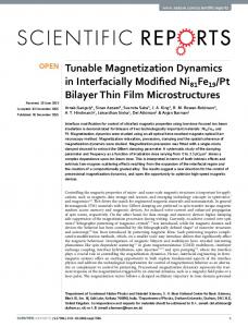
Figure 1. SPC-induced steady-state magnetization precession for elliptical Py particles (MS = 800 G, A = 1.3 × 10⁻⁶ erg cm−1 ) with thickness h = 3 nm and various lateral sizes as indicated in the legend. External field Hx = 1000 Oe is directed along the long ellipse axis. Upper panels: 3D trajectories of the average magnetization and typical domain pattern; lower panels: power spectra of mx -oscillations.
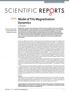
Another important fact demonstrated in [18] is that very similar power spectra and even very similar trajectories of the average magnetization can be observed for entirely different mesoscopic magnetization patterns. In particular, we have shown that sharp spectral peaks at almost the same frequency (corresponding to very similar so-called ‘butterfly’ trajectories of the average magnetization, see [18] for a detailed explanation) can be caused either by the ‘breathing’ (relatively slow movements) of smooth corner quasidomains or by the motion of a sharp domain wall across the element—dependent on the element size. This means that a small linewidth and a specific frequency value alone are not sufficient to identify which type of magnetization oscillation is observed in a nanoelement. The next question is the shape dependence of the limiting size for the validity of the macrospin approximation. The initial magnetization configuration (in the absence of a SPC) is more macrospin-like when the internal field is more homogeneous. Hence we expect that for an elliptical element the transition from a macrospin to a multidomain behaviour occurs at larger sizes (compared with a rectangular element) due to a more homogeneous demagnetizing field inside an elliptical nanoelement. Results for nanoelements with magnetic parameters corresponding to Py shown in figures 1 and 2 confirm this suggestion. It is also clear that the dependence of the oscillation character on the element shape is very strong, e.g. magnetization oscillations for the 20×40 nm2 ellipse are completely regular, whereby oscillations for the rectangle having the same lateral sizes are close to becoming chaotic (compare corresponding spectra in figures 1 and 2). We conclude this section by mentioning two kinds of problems where the macrospin model is useless by its very nature. The first kind are the problems which involve the
studies of the Oersted field influence (sometimes also called Ampere field) on the SPC-driven magnetization dynamics. This current-induced field in spin-injection devices can be quite large (up to ∼100 Oe and more) due to high dc-current densities used to excite magnetization oscillations. Thus, the inclusion of this field may be really important by the theoretical analysis of the magnetization dynamics. However, for the macrospin model this field cannot be taken into account properly, because the Oersted field HOe is highly inhomogeneous within the nanoelement flooded by the current. Thus, HOe cannot be properly included in the macrospin model, because the macrospin assumption corresponds actually to a point dipole approximation. The second situation where the macrospin approach fails completely is the magnetization dynamics in the point contact geometry, where the exchange interaction of a ‘free’ layer area subject to the spin torque (under-contact area) with the rest of this layer is crucially important. This interaction, which is responsible, in particular, for the emission of spin waves by the point contact area, cannot be adequately taken into account in the macrospin approximation.
3. SPC-induced magnetization dynamics of the nanopillar devices The nanopillar device includes in its ‘minimal’ version a columnar multilayered metallic nanoelement, containing (i) a ‘fixed’ FM layer (which means that one has to apply a rather high torque to induce its magnetic excitations) working as a current spin polarizer, (ii) a spacer made of a nonmagnetic metal and (iii) a ‘free’ FM layer designed so that its magnetization can be excited relatively easily. The magnetization of a ‘fixed’ layer can be ‘immobilized’ with 4
J. Phys. D: Appl. Phys. 41 (2008) 164013
D V Berkov and N L Gorn
20 x 10 nm2
1.0
1.0 1.0
80 x 40 nm2
40 x 20 nm2
my
my
0.8
0.0
0.0
0.6 0.4
-0.5
-0.5 1.0 0.5 m x 0.0 -0.5
0.2
mz
0.0 0.4
0.0
-0.4
-0.8
my
0.5
0.5
-1.0
-1.0
mx
m
0.4
z
0.0
0.5
-0.4
-1.0
z
0.0
0.5
-0.4
0.0 -0.8
mx
m
0.4
1.0
-0.8
-0.5
1.0
0.0 -0.5 -1.0
-1.0
P(m x )
P(m x )
P(m x )
0.1
2 0.1
1
f (GHz)
f (GHz)
f (GHz) 0
0.0
0.0 0
5
10
15
20
0
5
10
15
20
0
5
10
15
20
Figure 2. The same as in figure 1 for rectangular nanoelements of different lateral sizes.
various methods, such as making this layer much thicker than the ‘free’ one, or using the FM material with a large magnetocrystalline anisotropy, or growing this layer on an antiferromagnet, which leads to the so-called ‘exchange bias’ effect. Applying a large external field, we can achieve that both layers—‘fixed’ and ‘free’—are magnetized in roughly the same direction. Then, if the current direction corresponds to the flow of electrons from the ‘free’ to the ‘fixed’ layer, the electrons reflected from the fixed layer have their preferable magnetic moment direction opposite to the fixed layer magnetization. Such electrons, reaching the free layer (which equilibrium magnetization is also opposite to their magnetic moment polarization), produce the torque acting on the free layer magnetization Mfree . This torque acts so as to align Mfree along the polarization direction of reflected electrons, i.e. to bring Mfree out of its equilibrium position, thus inducing spin waves in the free layer when the current strength is high enough to overcome the damping. In this section, we shall analyze two groups of experiments made on different nanopillar devices. We start with the exchange biased nanopillars used in the work of Krivorotov et al [19], because here the samples were thoroughly characterized, which allowed an accurate quantitative comparison with numerical simulations. The results of Kiselev et al [9], being also highly non-trivial, have been obtained on much poorer characterized samples, leaving much room for their interpretation [11], and will be considered later.
nanoelement multilayer IrMn/Py(4 nm)/Cu(8 nm)/Py(4 nm) with the nominal elliptical cross-section 130 × 60 nm2 . The idea to pin the lower Py layer using an AF layer made of IrMn allowed a large angle to be achieved between the equilibrium magnetization orientations of lower (fixed) and upper (free) Py layers in a moderate external field. For this reason the angle between the polarization direction of electrons reflected from the fixed layer and the equilibrium orientation of the free Py layers is significantly smaller than 180◦ . Hence the spin torque caused by these electrons on the free layer magnetization has approximately the same direction across the upper Py nanoelement, despite its initial magnetization configuration being slightly inhomogeneous (see [14] for a detailed explanation why this is not so when the current electron polarization is collinear with the average magnetization of a nanoelement). The following main features of the SPC-induced oscillations found in [19, 20] could be explained and partly quantitatively reproduced by our micromagnetic simulations: (a) rapid decrease in the oscillation frequency f with increasing current strength I after the oscillation onset, (b) several frequency jumps in the f (I )-dependence and (c) very narrow spectral lines with the linewidth varying nonmonotonically with current. Rapid initial decrease in the oscillation frequency after the oscillation onset is a non-linear effect due to the rapid growth of the oscillation amplitude with increasing current immediately above the critical current strength (‘stiff’ generation). In the geometry where the thin-film magnetization oscillates initially around the axis lying in the film plane, this nonlinearity leads to the frequency decrease, as explained analytically in [21]. A somewhat oversimplified way to understand why the frequency decreases with increasing
3.1. Exchange biased Py/Cu/Py nanopillar Experiments on exchange biased nanopillars reported by Krivorotov et al (see [19] for first results, [20] for a detailed analysis) were performed on the columnar 5
J. Phys. D: Appl. Phys. 41 (2008) 164013
D V Berkov and N L Gorn
edges is nearly zero. After the second jump oscillations become localized in all directions: magnetization oscillates significantly only in the central region of the ellipse. Analytical theory of the transition between non-linear differently localized modes in continuous systems with vector degrees of freedom is, to our knowledge, not available, so we cannot compare our simulations with any analytical model. An interesting confirmation of our interpretation of the frequency jumps comes from the experiment itself [20]. To explain this, we emphasize that the first jump is due to the transition between the delocalized and localized modes and the second jump marks the transition between two localized modes with different localizations only. Hence we suggest that the first transition should be a more stable feature of a real system, where the surface imperfection and corresponding inhomogeneities in the stray field may smear out the qualitative difference between modes with different localizations. And indeed, frequency jumps vary significantly from sample to sample, whereby the first jump is observed almost always, although at different currents (see figure 6 in [20]), but the second jump is often absent. And in real systems, one of the major differences between various samples is a very different quality of their side surface, whereby simulations were always performed for an element with perfect borders. Narrow spectral lines and non-monotonic dependence of the linewidth on the current strength observed experimentally are a direct consequence of strongly non-collinear initial magnetization orientations of the fixed and free magnetic layers due to the exchange biased fixed layer. As mentioned above, this non-collinearity resulted in the spin torque acting on all magnetic moments approximately in the same direction, thus preventing the system from transition to a chaotic oscillation regime (see section 3.2). Even for currents near the frequency jumps, where the mixing of at least two nonlinear modes should lead to a substantial line broadening, the line width did not exceed ∼250 MHz. For currents well before and between the jumps, the lines were as narrow as ∼10 MHz. Determination of a spectral linewidth in micromagnetic simulations is much more difficult than determination of the oscillation frequency itself. The reason is not only the evident circumstance that in order to measure a linewidth �f one has to simulate the magnetization dynamics for a time interval �t � 1/�f (so that for a line width �f = 10 MHz we have to cover an interval �t ∼ 1 µs—a very long time for Langevin dynamics simulations). The even more important reason is that for magnetic materials with small Gilbert damping thermal fluctuations provide a significant (and often—a dominant) contribution to the linewidth, thus forcing us to perform simulations at a finite temperature. Such simulations include the stochastic (thermal) field as an additional contribution to the total effective field in (1). This field is a time-dependent random quantity, which is δ-correlated in space and time [22] and hence it converts the deterministic equation of motion (1) into a stochastic one. From the mathematical point of view, this conversion halves the order of accuracy achieved by any given numerical integration scheme [23], thus strongly reducing (typically by an order of magnitude) the allowed integration time step. This, in turn, leads to a large increase
7
f, GHz
8
6 5 4 3
aJ
2 0.2
0.4
0.6
0.8
1.0
1.2
1.4
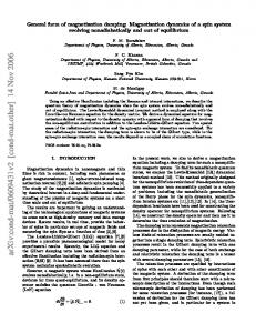
Figure 3. Simulated dependence of the oscillation frequency on the spin torque amplitude aJ with frequency jumps shown as dashed lines and spatial maps of the oscillation power (light means high oscillation power) showing different localization patterns of observed non-linear modes.
amplitude for this geometry is the qualitative analysis based on the expression f ∝ [H (H + 4πMeq )]1/2 for the in-plane oscillation frequency. Here the magnetization projection on the equilibrium direction of the magnetization Meq decreases with increasing oscillation amplitude (because the magnetization magnitude is conserved), thus leading to the frequency decrease. A remarkable feature of the nanopillar device studied in [19] is a very rapid frequency decrease with current after the oscillation onset, which shows that the oscillation amplitude (determined by the balance between the spin torque and damping) grows very fast with current at the initial stage. This rapid frequency decrease is reproduced very well by our simulations without any adjustable parameters, employing only the geometry and magnetic material properties measured independently. Frequency jumps in the f (I )-dependence are a much more intriguing feature. Macrospin model predicts that such jumps can occur in some situations [9] when the ‘smallangle’ elliptical precession orbit (linear regime) transforms into a ‘clam-shell’-like magnetization trajectory corresponding to strongly non-linear oscillations. However, on the one hand, micromagnetic simulations for the same geometry (see section 3.2) have shown that the macrospin approximation breaks down well before this transition should take place. Another argument against such a simple interpretation in our case is that already the first frequency jump (not to mention the second one) occurs in the deeply non-linear oscillation regime. Our simulations have demonstrated that these jumps are due to the transitions (mode hopping) between non-linear modes with different localization types. Up to the current corresponding to the first frequency jump magnetization oscillations are delocalized, i.e. magnetization everywhere within the nanoelement precesses with nearly the same amplitude (see figure 3). The first frequency jump manifests the transition to the mode which is localized in the direction along the long axis of the elliptical nanoelement, as it can be clearly seen from grey-scale maps in figure 3—oscillation amplitude of the 2nd mode near the ‘longitudinal’ element 6
J. Phys. D: Appl. Phys. 41 (2008) 164013
D V Berkov and N L Gorn
0.5
8
Sint
(a)
f, GHz
(b)
0.4
6
simulations 0.3 experiment
4 0.2 2
0.1 I, mA
0
I, mA
0.0 0
2
4
6
8
10
0
2
4
6
8
10
Figure 4. Comparison of the experimentally measured (�) and simulated (◦) current dependences of the oscillation frequency (a) and integrated rms-amplitude spectral density Sint (b).
in computational time corresponding to a given physical time interval. For these reasons we could provide only a semiquantitative comparison of our spectral linewidth ‘measurements’ with actual experimental data. First of all, we could confirm that the observed very small linewidth for all current values is due to the absence of quasichaotic dynamics for the geometry under consideration—magnetization oscillations remain regular up to the highest currents used experimentally. The reason for this behaviour is explained in the introduction to this section. Next, we were able to explain the non-monotonic linewidth dependence on the current. For currents only slightly above the oscillation onset threshold, thermal fluctuations play a relatively important role and lead to a significant broadening of spectral lines in the linear oscillation regime. When the current increases, the spin torque forces a rapid increase in the oscillation amplitude, whereas the contribution of thermal fluctuations grows much slower (only due to an approximately linear growth of the nanopillar temperature with current caused by the Joule heating). This leads to a decrease in the linewidth defined as a full width at half maximum (FWHM). By further increase in the current we approach the value for the first frequency jump, where the non-linear mode mixing (see above) leads to a less coherent magnetization configuration and thus—to an increase in the linewidth, which reaches its local maximum in the jump region. After the first frequency jump the linewidth decreases again when the first localized mode completely dominates the oscillations. For the same reason as for the first jump the linewidth increases again, approaching the current value for the 2nd inter-mode transition. After the 2nd transition the linewidth decreases for the same reason as for beyond the 1st jump, and finally increases because for the largest currents studied here the quasichaotic oscillations start to establish themselves. Detailed discussion of these issues is provided in [20]. As mentioned above, we could achieve a good quantitative agreement between simulated and measured frequencies (figure 4(a)), especially for small and moderate currents, where they nearly coincide (for large currents measured frequencies are systematically slightly lower than simulated ones; we shall return to this problem below). For this reason it is especially surprising that we observe a qualitative disagreement by comparing simulated and
measured oscillation powers (figure 4(b)): the measured power grows monotonically with current (except narrow current regions near the frequency jumps) and simulated power grows initially with current much faster than in a real experimental reaches its maximum for moderate current values and then slowly decreases. Taking into account that both power and frequency (for non-linear oscillations) are unambiguously related to the oscillation amplitude, the quantitative agreement for one of these quantities (frequency) and the qualitative disagreement for another one (power) is highly non-trivial. A possible explanation for such a situation could be that due to the imperfections of the specific nanopillar under study not the whole, but only a part of the free layer is oscillating for small currents, leading to a lower oscillation power than expected assuming the oscillations of the whole element. This could explain the slower initial increase in the power with current observed experimentally. Gradual oscillation onset of further parts of the free nanoellipse could account for a monotonic increase in the experimental power when the current is increased further. However, it is not clear at present, which sample imperfections could cause such behaviour. Another interesting discrepancy arises when one tries to include the effect of the dipolar interlayer interaction field, which in our case is not much smaller than the external field. In particular, Miltat has demonstrated (see results presented in [14]) that the inclusion of this interaction makes the agreement of the simulated frequency with experimental data worse. The reason for this behaviour is also not clear; to ‘rescue’ the good agreement achieved by the single-layer simulations presented above, one has to provide, e.g., good reasons why the dipolar interaction field is in practice much smaller then computed from the nominal experimental geometry. One of the reasons could be the imperfection of the element side border due to the patterning process; this process may not only introduce geometrical imperfections, but also decrease the magnetization near the border regions due to some oxidation. Further experiments on carefully characterized samples are obviously necessary to clarify this question. 3.2. Co/Cu/Co nanopillars in a longitudinal field Historically the paper of the Cornell group [9] devoted to the SPC-induced dynamics of a Co/Cu/Co multilayer structure 7
f, GHz
D V Berkov and N L Gorn
f, GHz
J. Phys. D: Appl. Phys. 41 (2008) 164013
Ms= 1400 G
Ms= 800 G
aJ
aJ (a)
(b)
Figure 5. Comparison of simulated magnetoresistance power spectra for elliptical nanoelements with different saturation magnetization values MS = 1400 G ((a) panel) and MS = 800 G ((b) panel). Other parameters: element thickness h = 3 nm, lateral size 130 × 70 nm2 , exchange stiffness constant A = 2 × 10⁻⁶ erg cm−1 , Gilbert damping parameter λ = 0.04. External field H0 = (Hx , Hy , Hz ) = (2000; 20; 100) Oe is directed approximately along the long ellipse axis which is chosen as x-axis.
was the first study where reliable data in the frequency domain concerning the steady-state microwave oscillations on a nanopillar device were reported. The structure used in [9] consisted of a ‘thick’ (40 nm) continuous Co layer separated by a 10 nm Cu spacer from a 3 nm thick elliptical Co nanoelement with nominal lateral size 130 × 70 nm2 . For the current direction corresponding to the electron flow from the upper (free) Co nanoelement to the lower (fixed) Co layer the authors of [9] could for the first time quantitatively study a steadystate magnetization precession (of a Co nanoellipse) detected as magnetoresistance oscillations in the GHz spectral band. All measurements have been done for the external field H0 directed approximately (but not exactly, what is important for the understanding of results) along the long axis of the free Co nanoellipse. Measuring the dependence of the oscillation frequency on the current strength, Kiselev et al have found very peculiar behaviour of the microwave spectrum of their Co/Cu/Co nanodevice. Namely, after the oscillation onset at I ≈ 1.8 mA a small-amplitude peak with a relatively large width and nearly constant frequency (fsm ≈ 16.5 GHz at H0 = 2 kOe) persisted up to I ≈ 2.4 mA, after which the frequency suddenly made a huge jump down to flr ≈ 4.5 GHz and the oscillation power increased by more than two orders of magnitude (large-amplitude regime). When the current was increased further, the central frequency of this huge broad peak with the linewidth ∼1 GHz slowly decreased until the signal disappeared at I ≈ 6 mA.
nanoellipse HK and the electron spin polarization degree P as fitting parameters, Kiselev et al succeeded in reproducing semiquantitatively both the small-amplitude signal with nearly constant frequency and the frequency jump from 16 to 4 GHz for current Ijump ≈ 1.14Ith , where Ith is the oscillation onset threshold. In this macrospin model the frequency of the small-amplitude oscillations is independent of current, because these oscillations correspond to the linear oscillation regime, where the frequency does not depend on the amplitude. The huge downward frequency jump corresponds to the transition between the small-angle elliptical magnetization orbit and the large-angle ‘clam-shell’-like orbits. Unfortunately, our full-scale micromagnetic simulations performed for various system parameters did not confirm this simple picture. Simulations of the experimental setup studied in [9] turned out to be laborious, because main parameters of the free magnetic layer were not known exactly and had to be determined by comparing simulation results with measurements. First of all, the saturation magnetization of Co within the (Cu/Co)n sandwich containing many 3 nm thick Co layers was measured as MS ≈ 800 G [9], which is much lower than the standard value MS (Co) ≈ 1400 G. The authors of [9] attributed this decrease to the influence of the surface anisotropy; however, such a drastic reduction of the saturation magnetization in a magnetic layer which is much thicker than the interatomic distance due to the surface anisotropy alone is quite unusual. Another possible reason for a smaller MS could be the nanoelement oxidation. Anyway, the exact value of the saturation magnetization of the oscillating layer was not known, so we have performed a separate study in order to find the influence of this parameter on the SPC-induced magnetization dynamics. One of our results on this behalf is shown in figure 5, where the oscillation spectra versus the spin torque amplitude aJ (which is proportional to the current strength I ) are shown for two different MS -values—standard MS (Co) ≈ 1400 G and the value MS ≈ 800 G reported in [9]. It can be seen that for currents (aJ values) just above sim ≈ 17 GHz the oscillation onset threshold the frequency fsm of simulated spectral peaks for MS ≈ 1400 G (figure 5(a))
3.2.1. Possible explanations for the origin and magnitude of the initial frequency jump. Although this non-trivial behaviour was not observed for all samples and the ‘smallangle’ signal frequency varied substantially from sample to sample [24], the understanding of this phenomenon was in the next few years the main subject of several theoretical studies, including both analytical theories and numerical simulations. The first attempt was made already by the Cornell group itself [9], who tried to fit the measured f (I ) dependence using macrospin simulations. Using the saturation magnetization MS and Gilbert damping λ of Co, anisotropy field of the 8
J. Phys. D: Appl. Phys. 41 (2008) 164013
D V Berkov and N L Gorn
uniaxial anis.
f, GHz
f, GHz
cubic anis.
aJ
aJ
(a)
(b)
Figure 6. Comparison of simulated magnetoresistance power spectra for elliptical polycrystalline nanoelements with average lateral grain size Dav = 10 nm ‘made of’ different crystalline modifications of Co: fcc Co with cubic magnetocrystalline anisotropy Kcub = 6 × 10⁵ erg cm−3 ((a) panel) and hcp Co with uniaxial magnetocrystalline anisotropy Kun = 4.5 × 10⁶ erg cm−3 ((b) panel). Magnetization MS = 800 G, exchange stiffness constant A = 3 × 10⁻⁶ erg cm−1 , other parameters as in figure 5. Grain anisotropy axes are randomly oriented in 3D.
reproduce quite well the experimental frequency of the ‘smallangle’ regime fsm ≈ 16.5 GHz. This is not surprising taking into account that this regime should correspond to the coherent magnetization oscillations of the whole nanoellipse and the basic FMR frequency for a thin Co layer with standard MS placed into the external field H0 = 2 kOe is fFMR ≈ 17.5 GHz. However, this is the only satisfactory agreement between simulations and experiment for MS ≈ 1400 G. Further increase in the current leads to a rapid loss of the magnetization coherence within the excited nanoelement, which results in a transition to quasichaotic oscillations accompanied by only a small downward frequency jump to fch ≈ 15 GHz, which is more than 3 times higher compared with the experimentally measured value of the ‘large-angle’ regime flr ≈ 4.5 GHz. Simulated oscillations for MS ≈ 800 G start at a lower sim frequency fsm ≈ 13.5 GHz due to the smaller saturation magnetization and jump to fch ≈ 10 GHz after transition to the quasichaotic regime, which is much closer to the experimentally observed value (still, the disagreement is too large to accept this result as a satisfactory one). Another important circumstance due to which we have finally adopted the value MS ≈ 800 G in our subsequent simulations is the relation of the current Iterm where detectable magnetization oscillations die off to the oscillations onset current Ith : in the real experiment (Iterm /Ith )exp ≈ 3, simulated value for MS ≈ 1400 G is (Iterm /Ith ) = (aterm /ath ) ≈ 6 and for MS ≈ 800 G we obtain (aterm /ath ) ≈ 4 (see figure 5). The reason why magnetization oscillations persist up to higher currents for the system with larger saturation magnetization is the stabilizing influence of the external field which prevents the magnetization of a nanoelement with higher MS from switching (or, as in our case, from a transition to the out-of-plane regime) up to larger current values. All in all, simulation results for MS ≈ 800 G reproduce the experimental picture definitely closer than those for MS ≈ 1400 G. Studying the influence of various material parameters on the magnetization dynamics, we have found a possible reason for the experimentally observed huge frequency jump. The reason proposed by us [11] is related to the existence of two crystallographic modifications of Co—fcc and hcp
structures, which can coexist in thin Co layers. The corresponding magnetocrystalline anisotropy of the cubic fcc Co (Kcub ≈ 6 × 10⁵ erg cm−3 ) is nearly an order of magnitude smaller than the uniaxial anisotropy of the hcp phase (Kun ≈ 4 × 10⁶ erg cm−3 ). Hence the influence of a random polycrystalline structure of a Co nanoellipse for the hcp material can be much stronger than for the fcc modification. To study this influence quantitatively, we have performed simulations of the SPC-induced dynamics for various nanoelement Co ‘samples’ with identical macroscopic parameters, but different realizations of their random polycrystalline structures with the same average grain size Dav = 10 nm. Indeed, we have found that for different random grain structures of the fcc Co oscillating spectra are quantitatively very similar (a typical example is shown in figure 6(a)). But for various ‘samples’ of the hcp Co the observed power phase diagrams on the (f –I )-plane were qualitatively different, as shown in figure 6 in our paper [11]. One example of the corresponding spectral plot is shown in figure 6(b), where several narrow spectral bands with large frequency jumps between them can be clearly seen for currents slightly above the oscillation onset threshold. These jumps correspond to the ‘migration’ of the oscillation power between different crystallites, where strongly different anisotropy fields lead to large differences in the oscillation frequency. Estimations given in [11] clearly show that a suitable realization of a random grain structure could be the reason for the huge frequency jump observed on a specific sample studied in figure 1 from [9]. This paradigm can also explain the large growth of the oscillation power after this jump found in [9]. Namely, we can assume that small MR-oscillations before the jump were due to the magnetization oscillations of one specific crystal grain only, whereas quasichaotic strong oscillations after the transition involve the magnetization of the whole or most of the nanoellipse. Our findings show once more that a careful and accurate characterization of the crystallographic structure of the samples under study is crucially important when dealing with SPC-induced oscillations, especially when dealing with 9
J. Phys. D: Appl. Phys. 41 (2008) 164013
D V Berkov and N L Gorn
value q1 = 1 the effect of the non-linearity should be really strong: the region of currents where the small-angle oscillations exist is strongly expanded and the subsequent frequency jump should be of the same order of magnitude as observed in [9] (we note in passing that by comparing their results to experimental data from [9] the authors of [27] have mistaken the second harmonic shown in figure 1(d) in [9] for the basic signal frequency). If they took the correct value from [9], the agreement between their simulations and experiment would become even better. To test this prediction of the non-linear damping model we have performed corresponding full-scale micromagnetic simu2 lations, including the first term λnl = λlin (1 + q1 (dm/dt)2 /ωM ) of a general non-linear damping (see above) in the LLGequation of motion (1). To keep the comparison with the macrospin model as ‘fair’ as possible we have included in our simulation neither the Oersted field nor the effect of the random crystal grain anisotropy, nor thermal fluctuations, thus simulating the ‘minimal’ micromagnetic model in the sense defined in [11, 20]. Corresponding results are presented in figure 7. Our results show that on the one hand, as expected, the current region (aJ in our simulations) where the linear oscillation regime exists after the oscillation onset and thus the oscillation frequency is current-independent, indeed expands with increasing non-linear dissipation parameter q1 . On the other hand, as can be seen from figure 7, full-scale micromagnetic simulations do not confirm the prediction of the macrospin model concerning the large magnitude of the frequency jump by the transition from ‘small angle’ (linear) to ‘large angle’ (non-linear) regime [27]. The oscillation frequency decreases indeed quite rapidly when the non-linear regime starts to establish itself. But due to the gradual loss of coherence of the magnetization configuration by increasing current the abrupt frequency jump for the studied q1 values is absent, and at the beginning of the quasichaotic regime the frequency is only about 10% smaller than the linear oscillation frequency. Oscillation power for this ‘minimal’ micromagnetic model demonstrates a very fast growth after the oscillation onset threshold, reaching its maximum when the transition from the linear to the regular (non-linear) largeangle oscillation regime is completed (compare figures 8(b) and (c)). When current increases further, the power falls off also very fast when the regular non-linear regime transforms into quasichaotic oscillations and then slowly decreases further (figure 8(a)). A very interesting feature of the observed non-linear magnetization dynamics is the emergence of the second oscillation mode by the transition from the linear to the nonlinear regular regime (seen as the upper frequency band in all plots in figure 7). The fraction of the oscillation power concentrated in this second mode grows rapidly with increasing non-linearity q1 , until for q1 = 2 this mode contains the major fraction of the oscillation power during the transition from the linear to the non-linear regime. Micromagnetic analysis reveals that this mode is localized in the central region of the nanoelement (upper grey-scale plot in the rightmost panel in figure 7), which explains why its frequency is higher than the frequency ‘basic’ mode which for the transition current
materials with a strong magnetocrystalline anisotropy such as Co or CoFe. A third explanation of the frequency jump was suggested by Montigny and Miltat [25] who have also performed fullscale micromagnetic simulations for a SPC-induced dynamics of s somewhat smaller (114 × 70 × 2.5 nm3 ) elliptical element. They have found that the mode arising first by the oscillations onset is localized near the ellipse edges and thus corresponds to the ‘edge mode’ discussed in [26]. The frequency of this mode was found to be nearly current independent, which is due to the fact that such an ‘edge mode’ is localized near the element edges where the demagnetizing field is especially large. When the current increases, the oscillation amplitude increases also, and the demagnetizing field decreases, because the average magnetization projection along the long ellipse axis (perpendicular to the edges where the mode is localized) becomes smaller. Thus the total field (Htot = Hext + Hdem ) acting on the magnetization near these edges increases, so that the frequency remains approximately constant despite the increasing oscillation amplitude. When the current increases further, a new mode arises according to simulations presented in [25], which is localized in the inner region of the ellipse and whose frequency decreases monotonically with current. The microwave power corresponding to this mode is significantly higher than for the edge mode, because the localization area of this ‘volume’ mode is much larger. So simulation results obtained in [25] could in principle also explain (at least qualitatively) experimental findings from [9]. However, we note that simulations in [25] have been performed for the exchange constant A = 1 × 10⁻⁶ erg cm−1 (a value typical for Py), which is 2–3 times smaller than exchange constants measured for Co (see our paper [11] for corresponding discussion). Such a relatively low exchange obviously assists the formation of the edge mode, allowing significant magnetization inhomogeneties already for small current values. In our simulations, where we have used the exchange A = (2–3) × 10−6 erg cm−1 , the first mode arising by the oscillation onset was always the homogeneous mode. Still, the explanation proposed in [25] cannot be excluded until reliable measurements of the exchange stiffness in thin Co films become available. The next possibility to explain the relatively wide region of currents where the small-angle oscillations exist and the subsequent frequency jump was suggested by Tiberkevich and Slavin [27], who have expanded the standard linear Gilbert model in order to account for the non-linear damping effects which must be present in real systems for magnetization oscillations with large magnetization change rate dm/dt or for large oscillation amplitudes. According to the theoretical analysis done in [27], non-linear effects can be taken into account by adding to the Gilbert damping λlin terms proportional to even powers of dm/dt, i.e. the non-linear damping, can be expressed 2 4 + q2 (dm/dt)4 /ωM + . . .), as λnl = λlin (1 + q1 (dm/dt)2 /ωM where ωM = 4π γ MS is the characteristic frequency. Phenomenological constants q1 , q2 , etc should be calculated from the microscopic theory for each specific damping mechanism. The macrospin model used in [27] to analyse the effect of these non-linear terms has shown that already for a moderate 10
J. Phys. D: Appl. Phys. 41 (2008) 164013
D V Berkov and N L Gorn
0.25
(a)
18 16
0.20
f , GHz
Figure 7. Simulated microwave spectra for linear (q1 = 0) and non-linear damping with various non-linearity parameters (q1 = 1 and q1 = 2). For the largest non-linearity q1 = 2 spatial distribution of the oscillation power (light contrast means high power) for two observed modes is shown.
(b)
14
q1 = 1
12 0 0.12
q1 = 2
0.10
0.2
0.05
aJ 0.14
0.16
0.18
P(mZ )
q1 = 0
P(mZ)
0.15
0.20
(c)
0.1
log(aJ)
0.00 0.1
1
0.0 0.12
aJ 0.14
0.16
0.18
0.20
Figure 8. Oscillation power as a function of the spin torque magnitude aJ for various non-linear damping parameters q1 as indicated in the legend. Panels (b) and (c), where the oscillation frequency and power for aJ values slightly above the excitation threshold are shown, demonstrate the correspondence between the transition from the linear to the regular non-linear regime and the maximal value of the oscillation power.
region is localized near the element edges: the demagnetizing field in the central region is lower, so that the total field (Htot = Hext + Hdem ) is higher, leading to the larger frequency of the ‘centred’ mode. The reason why the contribution of this second mode grows with the degree of non-linearity (q1 -value) is not completely clear. The ‘handwaving’ line of reasoning could be that the non-linear dissipation increase requires an opening of additional dissipation channels, and the mode under discussion can dissipate the energy more efficiently than the ‘basic’ mode due to its higher frequency. However, a rigorous analytical theory is required for a complete understanding of this phenomenon.
3 times higher than the experimental one (see figure 5(a)). Even when we adopt the much lower value MS = 800 G as suggested in [9], the discrepancy between simulations and experiment is by no means satisfactory (compare figure 5(b) with figure 1(f ) from [9]). This discrepancy is also unlikely to disappear if we assume that the Co samples studied experimentally had the hcp crystalline structure: we have simulated Nconf = 6 random realizations of the grain structure of Co nanoellipses (4 typical (f –I ) plots are shown in figure 6 in [11]) and the frequency at the beginning of the quasichaotic regime was never lower than fchsim ≈ 8 GHz, still being much exp higher than fch ≈ 4.5 GHz observed experimentally. We would like to point out that such a systematic difference between simulated and measured frequencies for large current values seems to be a robust feature: for exchange biased Py/Cu/Py nanopillar analysed in section 3.1, one can see from figure 4(a) that initially (for small currents) very good agreement between simulated and measured frequencies becomes systematically worse when the current increases. The agreement is also not getting better when one takes into account
3.2.2. Frequency of magnetization oscillations in the quasichaotic regime. A much more important question is the large disagreement between simulated and measured frequencies in the quasichaotic regime. We have already pointed out above that for the standard value of the Co magnetization (1400 G) the simulated frequency is more than 11
J. Phys. D: Appl. Phys. 41 (2008) 164013
D V Berkov and N L Gorn
the magnetodipolar interaction between the biased and free layers (see detailed analysis of this case in [14]). At the current state of the art, we can propose two explanations of this phenomenon. The first possibility is the systematic decrease in the saturation magnetization with increasing current due to the interaction of the spin-polarized electrons with the FM magnetization. Fundamental aspects of this inelastic spin torque are discussed from various points of view in [28, 29]. Such a decrease in MS , being proportional to the current strength, would nicely explain both the systematically higher simulated frequency and the growth of the difference between simulated and measured frequencies with increasing current. The second possibility would be the decrease in the exchange stiffness constant A with increasing current strength. Such a decrease would lead after the transition to the quasichaotic regime to a more inhomogeneous magnetization configuration than obtained in micromagnetic simulations where the current-independent exchange is used. For such more inhomogeneous magnetization states the observed average precession frequency would be lower for reasons discussed in section 3.1 of [11]. On this behalf we would like to draw the reader’s attention to the simulation results from the already cited paper [25], where simulations of the SPC-induced dynamics were performed for the nanoellipse with MS = 800 G (as in our paper [11]), but A = 1.0 × 10⁻⁶ erg cm−1 , which is much lower than the commonly accepted value for Co A = (2–3) × 10−6 erg cm−1 used by us. Simulated frequency at the beginning of a largeangle (probably quasichaotic) regime in [25] is ≈6 GHz, which is quite close to the value experimentally measured in [9].
coefficient D can be calculated for the known magnetic parameters very precisely [30]. For the point contact with the nominal diameter dc = 40 nm attached to the 5 nm thick Py thin film with the magnetization 4π MS = 8 kG (MS = 640 G), exchange stiffness A = 1.0 × 10⁻⁶ erg cm−1 placed into the in-plane external field H0 = 1000 Oe used in [31], one obtains analytically for the oscillation frequency fan = 2π ω0 ≈ 12 GHz, whereas the experimental value was fexp ≈ 7.7 GHz. The qualitative problem was that this measured frequency was well below even the basic (homogeneous) resonance frequency f0 ≈ 8.4 GHz, so that the measured magnetic excitations could not correspond to any kind of propagating wave. Numerical simulations of a point contact setup, where the extended thin film around the area flooded by a point contact is exchange coupled to the region under the contact and is thus an inherent part of the system to be simulated, are much more sophisticated than modelling of the nanopillar devices. The major difficulty here is due to the fact that the lateral size of a complete device (∼10–20 µm) is far above the size region accessible for numerical simulations on non-supercomputers, especially taking into account that discretization due to small sizes of the point contact itself should be fairly fine. Hence the simulated area should be restricted to the lateral sizes ∼1 × 1 µm2 , which for the small damping constants for commonly used magnetic material (λ ∼ 10−2 ) is insufficient to absorb the wave emitted by the under-contact region. For this reason this wave will be either reflected from (for open boundary conditions) or transmitted through (periodic BC) the borders of the simulated area, causing artificial interference effects with the primary wave, which are especially strong because these secondary waves have the same frequency. Additional difficulty arises if the border of the current-flooded area is cut off sharply, and a similar problem is caused by the calculation of the Oersted field. Methodical tricks to overcome these difficulties are explained in detail in [32], so now we turn to the further discussion of analytical and numerical progress in studying the magnetization dynamics in this geometry. The results of the first numerical simulation attempts, reported by us [33], were also in contradiction with the experiments of the NIST group [31]. Simulating magnetization dynamics by increasing current for a system with parameters adjusted to mimic the experimental setup of [31], we have found two steady-state oscillation modes (in contrast to only one mode observed in [31]). The simulated mode which appeared in our simulations [33] first by increasing the current strength was definitely the standard ‘linear’ mode predicted by Slonczewski [30], with the oscillation frequency being far above the measured one. When the current was increased above the second critical value, the under-contact area magnetization switched and started to precess around the direction opposite to the applied field. This second mode was localized and its frequency (not reported in [33]) was indeed below the basic FMR value for the system under study, being quite close to the measured value. However, neither the important contradiction with the experiment concerning the existence of the Slonczewski mode in our simulation could be resolved, nor was the nature of this localized mode understood in these first attempts.
4. Precession modes in the point contact geometry 4.1. Dynamics in a high external field Although a first theoretical study of the SPC-induced magnetization dynamics in the point contact setup was done by Slonzcewski already in 1999 [30], the first quantitative experimental results were obtained (to our knowledge) only five years later [31]. It was realized very quickly that experimental observations from [31] are in qualitative contradiction to theoretical predictions from [30]. The problem was not only that the critical current for the magnetic excitations threshold measured in [31] was substantially lower than predicted by Slonzcewski [30]; the estimation for this threshold contains some adjustable parameters and thus is in principle subject to debate. The much more serious disagreement was found between the predicted and observed frequencies of the magnetization oscillations. Namely, the oscillation mode predicted by Slonzcewski for the in-plane directed external field was a ‘normal’ propagating wave with the wavelength λ comparable to the point contact diameter dc = 2Rc , namely kc ≈ 1.2/Rc [30], where kc is the critical wave number. The corresponding oscillation frequency can then be calculated as ω =√ ω0 + Dkc2 , where both the basic FMR frequency ω0 = γ H0 (H0 + 4πMS ) and the spin-wave dispersion 12
J. Phys. D: Appl. Phys. 41 (2008) 164013
D V Berkov and N L Gorn
Important progress on this behalf was achieved by Slavin and Tiberkevich in [34], where they have shown that the mode observed in [31] corresponds to the so-called standing ‘bullet’, which is a non-linear self-localized excitation with a finite (and large!) oscillation amplitude already at the excitation threshold. This non-linearity causes a frequency shift towards lower frequencies, leading to the formation of the oscillation mode with frequency smaller than the basic FMR value f0 , which corresponds to the spatially localized excitation. This localization means that the radiation losses (which carry away most of the energy generated within the point contact area for the Slonczewski mode) are absent for this kind of mode. Hence its threshold excitation current Ithnl is smaller than for the Slonczewski mode, despite the initial ‘bullet’ oscillation amplitude being already large for I = Ithnl [34]. In numerical simulations (performed at T = 0) the ‘bullet mode’ for increasing current appeared, however, always after the linear Slonczewski mode, so that the prediction concerning its lower excitation threshold was still questionable. To resolve this difficulty, Consolo et al have studied the system behaviour by decreasing current [35]. Indeed, they have found that for this situation the ‘bullet’ mode persisted for currents below the critical current for the Slonczewski mode, thus confirming the analytical prediction from [34] about the ‘bullet’ excitation threshold. Essentially the same result was obtained in our paper [36], where we have found that when the current is increased, then at the current Itrans corresponding to the transition from the linear to the ‘bullet’ mode the average energy of the ‘bullet’ mode is significantly smaller than the energy of the linear Slonczewski mode. Hence we have suggested that already for currents significantly smaller than Itrans the linear mode is only metastable and that the ‘bullet’ mode is not observed for these smaller currents only due to the finite energy barrier, which must be surmounted to generate it. In a real experimental situation the energy required to overcome this barrier could be supplied by thermal fluctuations (we recall that measurements in [31] were performed at room temperature). Our numerical simulations have also revealed that the magnetization dynamics for the point contact geometry contains significantly more than a linear and one non-linear ‘bullet’ mode. Already for a very small point contact size dc = 40 nm used in [31] at currents much larger than the above mentioned value Itrans ≡ I (W → L1 ) for the transition from the linear propagating wave mode (W -mode) to the first localized mode (‘bullet’ or L1 -mode) we have detected another frequency jump (see figure 9(a)). This 2nd jump marks the transition from the ‘bullet’ mode to another type of a localized mode (L2 ), with a complicated core magnetization structure. Whereas the magnetization within the ‘bullet’ mode core is approximately homogeneous, the core dynamics of the 2nd localized mode is governed by the creation and annihilation of two vortex–antivortex pairs; corresponding grey-scale snapshots of the magnetization component perpendicular to the layer plane are shown in figure 9(a). Details of these non-trivial core structures together with the energy emission patterns of both localized modes (which are highly anisotropic) are discussed in [36].
Frequency f(mz), GHz
(a)
7.4 7.3
12
f, GHz
16
aJ
7.2
W
8
4.5
5.0
5.5
6.0
4
aJ
L1 0 0
4
6
7
L2
0.5
(b) Power
0.4 0.3 0.2 0.1
aJ
0.0 0
4
5
6
7
Figure 9. Oscillation frequency and power as functions of the spin torque magnitude aJ for the point contacts setup with parameters chosen to mimic the experiment from [31]: 5 nm thick Py thin film, MS = 640 G, A = 1.0 × 10⁻⁶ erg cm−1 , in-plane external field H0 = 1000 Oe.
We have also studied the system behaviour for increasing and decreasing currents (in our simulations this corresponds to increasing and decreasing spin torque amplitudes aJ ) for different values of the maximal current. Simulations were performed in the following way: for increasing current, the system was equilibrated at aJ = 0 and then the spin torque with the desired amplitude aJ (>0) was switched on instantaneously. This procedure was repeated for all aJ values to be studied; resulting frequencies and oscillation power as functions of aJ are shown in figures 10 and 11 as lines with open triangles (increasing aJ branches). For decreasing aJ values (decreasing current), after the initial system equilibration at aJ = 0 we have instantaneously increased aJ up to its maximal value aJmax (for the choice of this maximal value) see below and have allowed the steady state precession for this maximal current to establish itself, continuing dynamical simulations at aJ = aJmax for the time �t much larger than a precession period at aJmax , in our case—for �t = 5 ns. Then we have instantaneously decreased the spin torque amplitude down to the desired aJ value. Again, this procedure was repeated for all aJ values of interest; results are shown in figures 10 and 11 as lines with open circles. As can be seen, resulting dependences fincr (aJ ), Pincr (aJ ) and fdecr (aJ ), Pdecr (aJ ) all demonstrate a significant hysteresis, i.e. the dynamic behaviour of the system for increasing and decreasing currents is very different. Even more, this behaviour is qualitatively different depending on the maximal current value aJmax used for the rightmost point of the computed hysteresis loops. If we choose this maximal value aJmax smaller than the value aJ (L1 → L2 ) for the transition from the first (L1 ) to 13
J. Phys. D: Appl. Phys. 41 (2008) 164013
D V Berkov and N L Gorn
16
0.5 decr. aJ
(a)
14
(b)
incr. aJ
f, GHz
12 10 8
P, r.u.
0.4
0.3 0.2
6 4
0.1
2
aJ
aJ
0.0
0 2
3
4
5
6
2
7
3
4
5
6
7
Figure 10. Hysteretic behaviour of the oscillation frequency and power as functions of the spin torque magnitude aJ for the point contacts setup, when the maximal aJ value corresponds to the region where at increasing current the 1st localized mode still exists. 16
10 8
(b)
incr. aJ
0.4 0.3
P, r.u.
12
0.5 decr. aJ
(a)
f, GHz
14
0.2
6 4
0.1
2
aJ
0 3
4
5
6
aJ
0.0 3
7
4
5
6
7
Figure 11. The same as in figure 10 for the case when the maximal aJ value is chosen from the region where by increasing current the 2nd localized mode is generated.
onset (Ith ≈ 4 mA) and disappearance (Idp ≈ 8.5 mA) of magnetization oscillations found in [31]. Namely, we assume that the oscillation onset corresponds to the smallest value aJ,th ≈ 2.6 where the L1 -mode can exist (see the decreasing branch in figure 10) and the oscillation disappearance is due to the transition L1 → L2 at aJ,dp ≈ 6.25. Then the ratio of the upper and lower boundaries for the current region where the ‘bullet’ mode exists is aJ,dp /aJ,th ≈ 2.4. This value is surprisingly close to the experimental ratio Idp /Ith ≈ 2.1, taking into account that our simulations for this system do not include several important aspects of the real experimental situations (e.g. influence of the underlayer and presence of the Oersted field) and that several important parameters of the real system (e.g. the point contact diameter) are not known exactly. The hysteretic behaviour is also completely different when we increase the maximal current value up to aJmax = 7.0, thus including the existence region of the 2nd localized mode into the hysteresis loop (see figure 11). In this case when we decrease the current, the 1st localized mode is not observed at all. Instead, the L2 mode continues to exist well below the transition point L1 → L2 and even below the transition value aJ (W → L1 ) for the increasing current, occupying a significant current region where the linear Slonczewski mode exists on the increasing current branch. Only for a spin torque magnitude slightly above the excitation threshold for the linear mode, does the inverse transition L2 → W from the 2nd localized mode to the linear mode accompanied by the corresponding frequency jump take place as shown in 11(a). By further decreasing the current, this linear mode dies out in exactly the same manner as when the current is increasing.
the second (L2 ) localized modes at increasing current branch (in our case aJ (L1 → L2 ) ≈ 6.25), then the hysteresis looks as shown in figure 10, where we have chosen aJmax = 6.0. When the current increases from 0 to aJmax , the dependences fincr (aJ ) and Pincr (aJ ) reproduce, of course, corresponding curves already shown in figure 9 with the transition from the linear W to the 1st localized mode L1 at aJ (W → L1 ) ≈ 4.45. When the current is then decreased from its maximal value aJmax = 6.0, then the 1st localized mode is observed not only in the region where for the increasing branch the W -mode was present, but down to current values aJ significantly lower lin , in accordance than the linear mode excitation threshold aJ,th with the analytical prediction from [34] (as mentioned above, an analogous result was obtained for a system with another parameter in [35]). The presence of the 2nd localized mode, however, changes the behaviour of our system qualitatively. One important point is that the transition L1 → L2 allows us to explain the disappearance of magnetization oscillations observed in [31] for currents approximately twice the excitation threshold: if the mode detected in [31] was indeed the 1st localized (‘bullet’) mode found in our simulations, then the transition L1 → L2 to the 2nd localized mode could be interpreted experimentally as the disappearance of magnetization oscillations, because due to the highly inhomogeneous magnetization configurations of the L2 -mode core, the oscillation power of the 2nd mode P (L2 ) (averaged over the point contact area) is nearly an order of magnitude smaller than P (L1 ). Hence this mode could probably not be detected experimentally. We also note that combining the results shown in figures 9 and 10, we could reproduce quite well the relation between the currents for the 14
J. Phys. D: Appl. Phys. 41 (2008) 164013
D V Berkov and N L Gorn
However, a careful examination of this last transition L2 → W reveals that it is not accompanied by the jump in the oscillation power (figure 11(b)). This means that the position and even the very existence of this transition should be quite sensitive to the details of how the inverse hysteresis branch (decreasing current) is simulated. Indeed, we have found that when we decrease the spin torque magnitude from its maximal value aJmax = 7.0 to the specific value aJ under study, not instantaneously, but linearly with time, the current value where the inverse transition L2 → W occurs depends on the time interval used to decrease aJ . We note that in a real physical situation the time which passes between two subsequent current values used for magnetization oscillation measurements when current is decreased, is normally macroscopically large. For this reason further numerical studies in order to minimize the simulation time (still obtaining reliable and physically meaningful results!) are required.
(1)
(2)
(3)
(4)
Figure 12. Simulated spectral power versus current for the point contact geometry with a large contact diameter (dc = 80 nm) in a low external field H0 = 30 Oe. Arrows indicate the current values for which magnetization dynamics is shown in detail in figures 13–16.
4.2. Dynamics in a low external field Another interesting problem is the magnetization dynamics in a point contact setup in low external fields. In the absence of the stabilizing influence of a relatively large (∼1–10 kOe) applied field used in most experiments, one would expect, first of all, a larger variety of non-linear oscillation modes. Several interesting experimental results for such a situation have been reported very recently in [37], where magnetoresistance measurements in devices with the point contact diameters dc = 60–80 nm attached to a multilayer stack Co90 Fe10 (20 nm)/Cu(4 nm)/Ni80 Fe20 (5 nm) were performed. Applied field used in [37] was less than H0 < 50 Oe, which led to a qualitatively different dynamics compared with the previous high-field experiments of the same group [31]. The main result for the field-in-plane geometry was the discovery of an extremely low-frequency mode with f ≈ 200 MHz and several clearly visible harmonics. Experiments presented in [37] are even more challenging for numerical simulations than those considered above, because studying oscillations of such a low frequency requires simulations for long physical times. A further complication is the larger diameter of a point contact used in [37]. It results in a larger wavelength of the excited spin wave (compared with those studied in [31,32,36]), thus requiring a larger simulation area. Luckily, this increase in the point contact diameter simultaneously allows us to use larger discretization cells. We performed extensive numerical simulations of the experimental situation studied in [37], investigating the influence of the stray field of a ‘hard’ magnetic underlayer, the effect of its polycrystalline structure and the role of the Oersted field. Here we present only our preliminary results obtained for the simplest system consisting of a single Py layer only and neglecting the Oersted field effect. We are fully aware that the latter should play an important role especially in this case where the external field is weak, but the study of the ‘Oersted-field-free’ system is still a necessary first step to understand the system properties. Detailed simulation results including all the factors mentioned above will be presented elsewhere.
(a)
1.0
(c)
mX
0.5 0.0 -0.5
t, ns
-1.0 2.0
2.5
3.0
3.5
4.0
(b)
1.0
mZ
0.5 0.0 -0.5 -1.0 2.0
t, ns 2.5
3.0
3.5
4.0
Figure 13. Time dependences for in-plane magnetization projections mx (a), mz (b) and typical snapshots (c) of magnetization configurations (mz grey-scale maps) for the current value marked with the arrow (1) in figure 12.
Simulation results presented below are obtained on a single layer with the thickness h = 5 nm, to which a point contact with the diameter dc = 80 nm is attached. The lateral size of the simulation area is 2 × 2 µm2 , discretized laterally into 400 × 400 cells. Magnetic parameters are chosen as for the Py layer described in [37]: MS = 640 G, exchange stiffness A = 1×10⁻⁶ erg cm−1 , magnetocrystalline anisotropy of Py is neglected. Applied field H0 = 30 Oe is directed along the horizontal axis (with respect to the images shown in figures 13–16), chosen as the x-axis. The y-axis is perpendicular to the layer plane. The overall spectral power plot of mz -oscillations (in-plane magnetization projection perpendicular to the external field) versus current strength for the parameters given above is shown in figure 12. To calculate the absolute current 15
J. Phys. D: Appl. Phys. 41 (2008) 164013
D V Berkov and N L Gorn
(c) 1.0
(a)
mX
0.5
0.0
-0.5
t, ns -1.0 10
11
12
13
14
15
16
1.0
(b)
mZ
0.5
0.0
-0.5
t, ns
-1.0 10
11
12
13
14
15
16
Figure 14. Magnetization dynamics presented in the same way as in figure 13 for the current value marked with the arrow (2) in figure 12(c). Magnetization snapshots are shown as maps where the colour (online) or greyscale (print) gives the in-plane magnetization direction according to the direction wheel shown on the right-hand side.
the ‘bullet’ mode). Instead, the dynamics of the 1st localized mode is governed by the rotation of one vortex–antivortex pair clearly seen in figure 14(c). The energy is emitted out of the contact area by creation and subsequent annihilation of another small vortex–antivortex dipole, as shown in the last three colour maps in figure 14(c). Further current increase leads to the appearance of an extremely complicated dynamical regime, whose quasiperiodic magnetization time dependences are shown in figure 15. In this case the mode core consists alternately of one or two vortex–antivortex pairs, and the energy is emitted after the annihilation of one of these pairs in the form of different solitons (see figure 15(c)). Finally, for the largest currents studied here (from ≈43 mA upwards), the mode with the lowest frequency f ≈ 300 MHz and a relatively simple dynamics is found: two vortex– antivortex pairs are created and annihilated simultaneously, emitting two solitons in opposite directions (figure 16(c)). The large oscillation period results from the slow process of the vortex–antivortex pair rotation, accompanied by the change in the vortex–antivortex distance and finally—their mutual annihilation. Due to a strongly simplified model and highly complicated dynamics only a qualitative discussion of the relation between our preliminary data and experimental results from [37] is possible. We would like to emphasize, first, that we observe magnetization dynamics at much higher currents (Isim ∼ 10–50 mA) than those reported in [37] (Iexp ∼ 5–15 mA). This is partially due to the neglect of the underlayer influence—we have found that inclusion of the hard magnetic layer into a simulated model can make the oscillation
strength from the spin torque magnitude aJ we have used the standard expression aJ = h ¯ · I · P /(2|e|MS2 · h · (π rc2 )) [7, 8], assuming the electron polarization degree P = 0.4. It can immediately be seen that the magnetization dynamics already for this simplified model is much more complicated than that for the large field case. We could observe at least four dynamic regimes, one of which corresponds to the propagating Slonczewski mode and another three—to various localized modes. Below we show the time dependences for both in-plane magnetization projections and typical snapshots of magnetization configurations for all four cases. The Slonczewski mode is again excited first, starting approximately at Ith ≈ 10 mA. An interesting feature of this mode in its deeply non-linear regime is the existence of strong higher harmonics, clearly visible in figure 13(c) as a modulation of the propagating wave amplitude (greyscale contrast) by excitations with smaller wavelength. The anisotropy of the wave velocity is also pronounced significantly stronger than for the small contact diameter (see the map for the W -mode in figure 9) due to a larger wavelength for the system under study. When the current is increased to ≈22 mA, a large frequency jump from ≈4.5 GHz down to ≈1.3 GHz occurs, signalling the excitation of the 1st localized mode. In contrast to the case studied in section 4.1, the ‘bullet’ mode with its approximately collinear magnetization core structure is not observed at all for the system simulated here. The absence of the ‘bullet’ mode is probably due to the larger contact diameter and lower field value compared with that used in section 4.1, because small contact diameter and large field should strongly ‘assist’ to form a homogeneous core magnetization state (as in 16
J. Phys. D: Appl. Phys. 41 (2008) 164013 1.0
D V Berkov and N L Gorn
the point contact is relatively large and the external field very small, the current-induced magnetic field (Oersted field) plays a qualitatively important role, completely changing the excitation spectrum, as we have found in our simulations (results not shown here). For this reason the inclusion and proper calculation of this field for the specific experimental setup is crucially important for understanding the SPC-induced magnetization dynamics under these conditions.
(c)
(a)
mX
0.5 0.0 -0.5
t, ns
-1.0 6
8
10
12
14
16
18
20
5. Conclusion 1.0
(b)
Our extensive full-scale micromagnetic simulations have shown that in the framework of the Slonczewski model one can explain, at least qualitatively, major important features of the SPC-induced magnetization dynamics in nanopillars, including frequency jumps and very different line widths for various oscillation regimes. Still, several important problems, first of all—a systematic difference between simulated and measured frequencies for this geometry—require further extensive study. For the point contact setup the situation is much more complicated, because the generation and interplay between various possible non-linear localized and delocalized oscillation modes is not understood satisfactorily even on the qualitative level. From the experimental side, precise characterization of each sample under study (or at least detailed reports about the material properties and sample to sample variation of results) together with the exact calculation of the Oersted field for each specific experimental setup are necessary to enable further progress.
mZ
0.5 0.0 -0.5 -1.0
t, ns 6
8
10
12
14
16
18
20
Figure 15. The same as in figure 14 for the current marked with the arrow (3) in figure 12(c). (c) 1.0
(a)
mX
0.5 0.0 -0.5
Acknowledgment t, ns
-1.0 11
12
13
14
15
The authors thank the German Research Society for its support in framework of the SPP 1133 ‘Ultrafast magnetization dynamics’ (project BE 2464/4).
16
1.0
(b) 0.5
mZ
References 0.0
[1] Slonczewski J C 1996 Current-driven excitation of magnetic multilayers J. Magn. Magn. Mater. 159 L1–7 [2] Berger L 1996 Emission of spin waves by a magnetic multilayer traversed by a current Phys. Rev. B 54 9353 [3] Kronm¨uller H and Parkin S (ed) 2007 Handbook of Magnetism vol 2 (New York: Wiley) [4] Waintal X et al 2000 Role of spin-dependent interface scattering in generating current-induced torques in magnetic multilayers Phys. Rev B 62 12317 Stiles M D and Zangwill A 2002 Anatomy of spin-transfer torque Phys. Rev. B 66 014407 Slonczewski J C 2002 Currents and torques in metallic magnetic multilayers J. Magn. Magn. Mater. 247 324 Xiao J, Zangwill A and Stiles M D 2004 Boltzmann test of Slonczewski’s theory of spin-transfer torque Phys. Rev. B 70 172405 Berger L 2005 Relation between giant magnetoresistance and critical current for spin precession in magnetic multilayers Phys. Rev. B 72 R-100402 Kim J-V 2006 Stochastic theory of spin-transfer oscillator linewidths Phys. Rev. B 73 174412 [5] Kiselev S I, Sankey J C, Krivorotov I N, Emley N C, Schoelkopf R J, Buhrman R A and Ralph D C 2003
-0.5
t, ns
-1.0 11
12
13
14
15
16
Figure 16. Magnetization dynamics for the high-current (arrow (4) in figure 12(c)) steady-state precession regime presented in the same way as in figure 14.
onset threshold up to 2 times smaller. Further reduction in the onset current may be due to the inhomogeneities of the hard layer stray field due to its random grain structure. Corresponding results shall be discussed in detail elsewhere. Second, we have shown that the extremely low (for the SPCinduced dynamics, of course) frequency observed in [37] may be due to the rotation and creation–annihilation process of the vortex–antivortex pairs. And the last important point is that for the situation under study, where the diameter of 17
J. Phys. D: Appl. Phys. 41 (2008) 164013
[6] [7] [8] [9]
[10] [11] [12] [13] [14] [15] [16] [17]
[18]
[19]
D V Berkov and N L Gorn
[20] Krivorotov I N, Berkov D V, Gorn N L, Emley N C, Sankey J C, Ralph D C and Buhrman R A 2007 Large-amplitude coherent spin waves excited by spin-polarized current in nanoscale spin valves Phys. Rev. B 76 024418 [21] Slavin A N and Kabos P 2005 Approximate theory of microwave generation in a current-driven magnetic nanocontact magnetized in an arbitrary direction IEEE Trans. Magn. MAG-41 1264 [22] Brown W F 1963 Thermal fluctuations of a single-domain particle Phys. Rev. 130 1677 [23] Kloeden P E and Platen E 1995 Numerical Solution of Stochastic Differential Equations (Berlin: Springer) [24] Kiselev S 2005 private communication [25] Montigny B and Miltat J 2005 Micromagnetic simulations of current-induced microwave excitations J. Appl. Phys. 97 10C708 [26] Bayer C et al 2005 Spin-wave excitations in finite rectangular elements of Ni80Fe20 Phys. Rev. B 72 064427 [27] Tiberkevich V and Slavin A 2007 Nonlinear phenomenological model of magnetic dissipation for large precession angles: generalization of the Gilbert model Phys. Rev. B 75 014440 [28] de Loubens G, Naletov V V and Klein O 2005 Reduction of the spin-wave damping induced by nonlinear effects Phys. Rev. B 71 180411(R) [29] Takacs A F, Balashov T, Dane M, Ernst A, Bruno P and Wulfhekel W On the relation of the inelastic spin torque and the spin polarisation Phys. Rev. Lett. submitted [30] Slonczewski J C 1999 Excitation of spin waves by an electric current J. Magn. Magn. Mater. 195 L261 [31] Rippard W H, Pufall M R, Kaka S, Russek S E and Silva T J 2004 Direct-current induced dynamics in Co90 Fe10 /Ni80 Fe20 point contacts Phys. Rev. Lett. 92 027201 [32] Berkov D V and Gorn N L 2006 Micromagnetic simulations of the magnetization precession induced by a spin polarized current in a point contact geometry J. Appl. Phys. 99 08Q701 [33] Berkov D V and Gorn N L 2004 Invited talk 053-HP Joint European Magnetic Symp. (Dresden, Germany, September 2004) Berkov D V and Gorn N L 2005 Invited talk 28TL-D-6 Moscow Int. Symp. on Magnetism (Moscow, Russia, June 2005) Berkov D V 2006 Micromagnetic simulations of the magnetization dynamics in nanostructures with special applications to spin injection J. Magn. Magn. Mater. 300 159 [34] Slavin A and Tiberkevich V 2005 Spin wave mode excited by spin-polarized current in a magnetic nanocontact is a standing self-localized wave bullet Phys. Rev. Lett. 95 237201 [35] Consolo G, Azzerboni B, Gerhart G, Melkov G A, Tiberkevich V and Slavin A N 2007 Excitation of self-localized spin-wave ‘bullets’ by spin-polarized current in in-plane magnetized magnetic nano-contacts: a micromagnetic study Phys. Rev. B 76 144410 [36] Berkov D V and Gorn N L 2007 Magnetization oscillations induced by a spin-polarized current in a point-contact geometry: mode hopping and non-linear damping effects Phys. Rev. B 76 144414 [37] Pufall M R, Rippard W H, Schneider M L and Russek S E 2007 Low-field current-hysteretic oscillations in spin-transfer nanocontacts Phys. Rev. B 75 140404(R)
Microwave oscillations of a nanomagnet driven by a spin polarized current Nature 425 380 Kiselev S I, Sankey J C, Krivorotov I N, Emley N C, Garcia A G F, Buhrman R A and Ralph D C 2005 Spin-transfer excitations of permalloy nanopillars for large applied currents Phys. Rev. B 72 064430 Krivorotov I N, Emley N C, Sankey J C, Kiselev S I, Ralph D C and Buhrman R A 2005 Science 307 228 Mistral Q, Kim J-V, Devolder T, Crozat P, Chappert C, Katine J A, Carey M J and Ito K 2006 Current-driven microwave oscillations in current perpendicular-to-plane spin-valve nanopillars Appl. Phys. Lett. 88 192507 Acremann Y, Strachan J P, Chembrolu V, Andrews S D, Tyliszczak T, Katine J A, Carey M J, Clemens B M, Siegmann H C and St¨ohr J 2006 Time-resolved imaging of spin transfer switching: beyond the macrospin concept Phys. Rev. Lett. 96 217202 Sankey J C, Braganca P M, Garcia A G F, Krivorotov I N, Buhrman R A and Ralph D C 2006 Spin-transfer-driven ferromagnetic resonance of individual nanomagnet Phys. Rev. Lett. 96 227601 Tserkovnyak Y, Brataas A, Bauer G E W and Halperin B I 2005 Nonlocal magnetization dynamics in ferromagnetic heterostructures Rev. Mod. Phys. 77 1375 Stiles M D and Miltat J 2006 Spin Transfer Torque and Dynamics Spin Dynamics in Confined Magnetic Structures III ed B Hillebrands and A Thiaville (Berlin: Springer) Xiao J, Zangwill A and Stiles M D 2005 Macrospin models of spin transfer dynamics Phys. Rev. B 72 014446 Kiselev S I, Sankey J C, Krivorotov I N, Emley N C, Schoelkopf R J, Buhrman R A and Ralph D C 2003 Microwave oscillations of a nanomagnet driven by a spin polarized current Nature 425 380 Sun J Z 2000 Spin-current interaction with a monodomain magnetic body: a model study Phys. Rev. B 62 570 Berkov D V and Gorn N L 2005 Magnetization precession due to a spin-polarized current in a thin nanoelement: numerical simulation study Phys. Rev. B 72 094401 Li Z and Zhang S 2003 Magnetization dynamics with a spin-transfer torque Phys. Rev. B 68 024404 Hubert A and Sch¨afer R 1998 Magnetic Domains: The Analysis of Magnetic Microstructures (Heidelberg: Springer) Berkov D V and Miltat J 2008 Spin-torque driven magnetization dynamics: micromagnetic modelling J. Magn. Magn. Mater. 320 1238 Katine J A et al 2000 Current-driven magnetization reversal and spin-wave excitations in Co/Cu/Co pillars Phys. Rev. Lett. 84 3149 Grollier J et al 2001 Spin-polarized current induced switching in Co/Cu/Co pillars Appl. Phys. Lett. 78 3663 Acremann Y, Strachan J P, Chembrolu V, Andrews S D, Tyliszczak T, Katine J A, Carey M J, Clemens B M, Siegmann H C and St¨ohr J 2006 Time-resolved imaging of spin transfer switching: beyond the macrospin concept Phys. Rev. Lett. 96 217202 Berkov D V and Gorn N L 2005 Transition from the macrospin to chaotic behavior by a spin-torque driven magnetization precession of a square nanoelement Phys. Rev. B 71 052403 Krivorotov I N, Emley N C, Sankey J C, Kiselev S I, Ralph D C and Buhrman R A 2005 Science 307 228
18