non-negative matrix factorization and classifiers - ee.oulu.fi
Recommend Documents
Suppose one wants to model moustaches and beards of a database of human faces with. 4 parameters. The first parameter represents the top of the moustache ...
ristretto, written in Python, which allows the reproduction of all results (GIT .... decomposition of Y is used to form a matrix Q â RmÃk with orthogonal ...... database of handwritten digits, which comprises 60,000 training and 10,000 ... Table 4
ABSTRACT. We address the problem of blind audio source separation in the under-determined and convolutive case. The cont
Nov 5, 2014 - are from Wallflower [40]. The first row image sequences are from [21]. include each image frame as a rank and thus it cause dense basis matrix ...
perimental results on real-world datasets show that our method has strong perfor- ..... other hand, some other methods can find more accurate results but require .... 11K. 0.80. 0.82. 0.80. 0.77. 0.80 0.86. 0.82. 0.52. 0.80. 0.87. PROTEIN. 18K.
However, most of the existing NMF algorithms do not pro- vide uniqueness of the ..... Second, the Welch's method is applied to calculate the .... (where â and â denote the elementwise multiplication and division, respectively), it is obvious that
Department of Information and Computer Science. â. Aalto University School of Science and Technology. P.O.Box 15400 ... Nonnegative learning based on matrix factorization has received a lot ...... Mathematical Forum, 3:1853â1870, 2008.
Sep 22, 2017 - methods to fuse hyperspectral data and high spatial resolution .... Remote Sens. , vol. 43, pp. 455-465, 2005. N. Yokoya, C. Grohnfeldt, and J. Chanussot, "Hyperspectral and ... Geoscience and Remote Sensing Magazine, vol.
Exploratory Multi-way Data Analysis and Blind Source Separation,. Wiley, 09 ..... Proc. of the 8th IEEE Int. Conf. on Data Mining (ICDM), pp. 353-362, 2008.
... HUT, Finland. E-mail: {zhijian.yuan, zhirong.yang, erkki.oja}@hut.fi ... The close relation of NMF to clustering has been shown by Ding et al [4]. For recent ...
value decomposition and nonnegative matrix factorization for the purpose of ... topic that has been used. Nirmal Thapa is with Department of Computer Science, University of .... Mathematical derivation for update formula. Let,. Q = A â HW2. F.
This work was supported in part by the National Science Foundation. ... Nonnegative Matrix Factorization: Algorithms and Applications ... Math, Georgia Tech.
iments on 5 real-life datasets show relations between NMF and PLSI ... (physical) representation of the given data set;
[email protected]. School of Computational Science and Engineering. Georgia Institute of Technology .... Other rank-1 downdating based algorithms (Vavasis,..) C. Ding, T. Li, ...... Georgia Tech. Prof. Tao Li CS, Florida International Univ.
imaging (CSI), hierarchical decomposition, magnetic resonance. (MR), magnetic ... lege of New York, New York, NY 10031 USA (e-mail: [email protected]).
Feb 10, 2010 - Representation of convolutive mixing system and formulation of Multichannel NMF problem. ...... vibrato). The EM and MU algorithms were run for 500 itera- ... guitar) is recorded with several microphones placed close to.
Abstract+An activeSperiodSaware supervised nonnegative maS trix factorization (NMF) approach for music transcription is proposed. supervised NMF relies on ...
Therefore, data-driven dictionary is introduced into sparse representation [22]. Dictionary learning ... Multi-task learning is a type of machine learning that learns.
Sep 19, 2016 - Facebook ..... OF GTNMF CO MPAR ED TO S EVE RA L NMF APP ROAC HES . ..... ternational ACM SIGIR conference on Research and development in .... [21] U. Von Luxburg, âA tutorial on spectral clustering,â Statistics and.
SSNMF can use the (partial) class label explicitly, serving as semi-supervised feature .... 1) Document Data Matrix: In the vector-space model of text data, each ... the power spectral density (PSD) in the band 8â30 Hz every. 62.5 ms, (i.e., 16 ...
Nov 3, 2011 - (MC)jSj Ti (MR)i = M ...... Say a row Mj is a loner if (ignoring other rows that are copies of Mj) it is .... For a row M j, we call it a robust-loner if upon.
and Saul, 2000] [Niyogi, 2003]. Yet NMF does not exploit ..... J. H. Friedman. ... Saul. Nonlinear dimensionality reduction by locally lin- ear embedding. Science ...
non-negative matrix factorization and classifiers - ee.oulu.fi
email: [email protected].fi ..... in Rr. Unlike JAFFE16, it is hard to say here when NMF could be used ... and hard to classify: accuracies achieved in [10] with Ker-.
NON-NEGATIVE MATRIX FACTORIZATION AND CLASSIFIERS: EXPERIMENTAL STUDY Oleg G. Okun Machine Vision Group Infotech Oulu and Department of Electrical and Information Engineering P.O.Box 4500, FIN-90014 University of Oulu, FINLAND email: [email protected] ABSTRACT Non-negative matrix factorization (NMF) is one of the recently emerged dimensionality reduction methods. Unlike other methods, NMF is based on non-negative constraints, which allow to learn parts from objects. In this paper, we combine NMF with four classifiers (nearest neighbor, kernel nearest neighbor, k-local hyperplane distance nearest neighbor and support vector machine) in order to investigate the influence of dimensionality reduction performed by NMF on the accuracy rate of the classifiers and establish when NMF is useless. Experiments were conducted on three real-world datasets (Japanese Female Facial Expression, UCI Sonar and UCI BUPA liver disorder). The first dataset contains face images as patterns whereas patterns in two others are composed of numerical measurements not constituting any real physical objects when assembled together. The preliminary conclusion is that while NMF turned out to be useful for lowering a dimensionality of face images, it caused a degradation in classification accuracy when applied to other two datasets. It indicates that NMF may not be good for datasets where patterns cannot be decomposed into meaningful parts, though this thought requires further, more detailed, exploration. As for classifiers, k-local hyperplane distance nearest neighbor demonstrated a very good performance, often outperforming other tested classifiers. KEY WORDS Dimensionality reduction, pattern classification, machine learning.
1 Introduction Pattern classification is one of the final operations in the object interpretation and recognition process. Operations preceding to it influence on classification results and therefore selection of appropriate preprocessing techniques is of great importance. An almost unavoidable choice for a preprocessing operation includes dimensionality reduction, since it can reduce the negative effect known as curse of dimensionality. Though it seems that dimensionality reduction followed by classification has been studied for various combinations, we selected a relatively new technique called
non-negative matrix factorization [1] and combine it with four advanced classifiers (nearest neighbor, kernel nearest neighbor, k-local hyperplane distance nearest neighbor and support vector machine) in order to find out how NMF influences on the classification error rate. Since its first appearance, NMF and its modifications were studied in a number of works [2, 3, 4, 5, 6, 7, 8], where NMF was applied for image retrieval and classification. However, usefulness of NMF for general object classification (when objects are not images, but rather sets of numerical features, e.g. measurements), was not yet verified. In this paper, we therefore explore this aspect in order to find out if NMF can bring improvements to classification accuracy, even if its definition does not suggest such kind of application. Moreover, all (except nearest neighbor) the selected classifiers were not used with NMF to our best knowledge. Thus, we extend research concerning coupling NMF with different classifiers with the goal to determine appropriate ones. The paper has the following structure. Sections 2 and 3 briefly describe the non-negative matrix factorization and four classifiers, respectively. Experiments are presented in Section 4. Finally Section 5 concludes the paper.
2 Non-negative Matrix Factorization (NMF) Non-negative matrix factorization is a linear dimensionality reduction technique which is distinguished from such methods as PCA by its non-negativity constraints. These constraints lead to a part-based representation because they allow only additive, not subtractive, combinations. Given a non-negative n × m matrix V (m vectors, each of n elements), NMF finds a non-negative n×r matrix W and a non-negative matrix r × m matrix H such that V ≈ WH. The value of r is selected according to the rule nm r < n+m in order to obtain dimensionality reduction. Each column of W is a basis vector while each column of H is a reduced representation of the corresponding column of V. In other words, W can be seen as a basis that is optimized for linear approximation of the data in V. NMF provides the following simple learning rule guaranteeing to monotonically converge without the need
for setting any adjustable parameters [1]: Wia ← Wia
X µ
Haµ
Viµ Haµ , (W H)iµ
Wia Wia ← P , j Wja X Viµ . ← Haµ Wia (W H)iµ i
(1)
(2) (3)
The matrices W and H are initialized with positive random values. Equations (1-3) iterate until convergence to a local maximum of the following objective function: F =
n X m X
(Viµ log(W H)iµ − (W H)iµ ) .
(4)
i=1 µ=1
In its original form, NMF can be slow to converge to a local maximum for large V. We found that introducing a parameter tol (0 < tol 1) to decide when to stop iterations significantly speeds up the convergence (from several hours to several minutes) without degrading the approximation quality. This is also in accordance with information retrieval results in [2], where the average precision remained almost the same as the number of iterations increased. After learning the NMF basis functions, i.e. the matrix W, new data are projected into r dimensional space by fixing W, randomly initializing H as described above, and iterating (1-3) until convergence [3].
3 Classifiers 3.1 K Nearest Neighbor (KNN)
only determined by the support vectors which are a subset of the training data so that the solution is often very sparse. Another advantage of SVM is that its solution does not depend on a data dimensionality, unlike that of many other methods, and this makes it an attractive choice for dealing with high dimensional datasets. Given that the data cannot be always linearly separated in an input space, SVM performs their mapping into another, a higher dimensional feature space where the data are supposed to be linearly separated. So called “kernel trick” allows not to calculate this mapping explicitly. Instead, the mapping into the feature space is implicitly defined by a kernel function computing the inner product of two feature vectors corresponding to two inputs. In some cases, if the data are noisy, there can be no linear separation in the feature space. To deal with this obstacle, the following (dual) optimization problem is to be solved1 : maximizeP Pm m W (α) = i=1 αi − 21 i,j=1 yi yj αi αj K(xi , xj ) , subject Pm to i=1 yi αi = 0 , 0 ≤ αi ≤ C, i = 1, . . . , m , (5) where αi are Lagrange multipliers, K(xi , xj ) is a kernel value for inputs xi and xj that correspond to outputs yi and yj , and C is the trade-off between minimizing the number of training errors and maximizing the margin (classifier capacity). Given a test point x, the nonlinear SVM classifier takes the form2: f (x) =
m X
αi yi K(x, xi ) + b ,
i=1
There is no training step and classification of unseen points is simple. K nearest neighbors are sought for each test point among members of the training set and a point in question is assigned to a class of majority neighbors. To avoid ties, K should be odd. Standard values for K are 1, 3 or 5 in order to keep the computational cost low.
3.2 Support Vector Machine (SVM) Unlike many traditional methods which implement the Empirical Risk Minimization Principle which aims at minimizing the training error, SVM implements the Structural Risk Minimization Principle [9] which seeks to minimize an upper bound of the generalization error, which eventually results in better generalization of SVM than that of traditional techniques. Currently, SVM is considered as the most advanced classifier which can outperform various models of neural networks in many practical tasks. The training of SVM is equivalent to solving a linearly constrained convex quadratic programming problem and therefore the solution of SVM is always globally optimal and free from local minima. In fact, the solution is
y(x) = sign(f (x)) ,
(6)
where the scalar b can be chosen so that yi f (xi ) = 1 for any i with 0 < αi < C.
3.3 Kernel Nearest Neighbor (KernelNN) This algorithm is a modification of the standard KNN when applying kernels [10]. When selecting an appropriate kernel, the kernel nearest neighbor algorithm, via a nonlinear mapping to a high dimensional feature space, may be superior over KNN for some sample distributions. The same kernels as in case of SVM are commonly used, but as remarked in [10], only the polynomial kernel with degree p 6= 1 is actually useful, since the polynomial kernel with p = 1 and radial basis kernel degenerate KernelNN to the conventional KNN. 1 We talk here and further in this section about 2-classes problems for simplicity. 2 In fact, since many α = 0, the actual upper summation limit is i (much) less than m. Points for which 0 < αi < C are called support vectors.
The kernel approach to KNN consists of two steps: kernel computation, followed by distance computation in the feature space expressed via a kernel K. After that, a nearest neighbor rule is applied just as in case of KNN. In (7), KernelNN redefines a distance metric for using in the feature space. d(φ(x), φ(y)) =
4 Experiments Four classifiers were applied to the data of the original and reduced dimensionality. The main goal of experiments was to verify the influence of NMF on the error rate of each classifier as well as to compare the classifiers between themselves.
p
K(x, x) − 2K(x, y) + K(y, y) , (7) where K(x, y) = hφ(x), φ(y)i and φ(x) is a mapping of x into the feature space. Similarly to SVM, the problem of choosing the optimal kernel and its parameters influences on the error rate. However, given the optimal kernel, results of KernelNN will be not worse than those of KNN, since KNN is a specific kind of KernelNN.
3.4 K-Local Hyperplane Distance Nearest Neighbor (HKNN) This algorithm was proposed in [11] in order to improve KNN in its competition with SVM. Unlike (nonlinear) SVMs which map the input data into a higher dimensional feature space and build a decision surface (hyperplane maximizing a margin) in this space, an alternative approach exploited in [11] is to construct a nonlinear decision surface directly in the input space. It is often convenient to consider each class as forming a low dimensional manifold embedded in a higher dimensional input space. This low dimensional manifold can be reasonably assumed locally linear. The reason why SVM often outperforms KNN is that in case of a finite number of samples, i.e. when data are relatively sparse, “missing” samples, appearing as “holes”, bring distortions (e.g. complicated nonlinearity leading to overfitting) to the decision surface produced by KNN3 , and this negatively affects generalization performance of KNN. The idea of HKNN is to fantasize the missing points to remedy this drawback. Given a test point, its K nearest neighbors, found among training points belonging to a certain class, approximately form the local hyperplane passing through them. Thus this hyperplane would include all the “missing” points of the manifold representing this class. Having such a hyperplane constructed for each class, a given test point x is assigned to the class whose hyperplane is closest to x. To compute a hyperplane, one needs to solve a small linear system (see [11] for details) so that the overall computational load is still low and comparable to that of KNN. Except K whose value should be typically larger than that in KNN (in order to have enough points for constructing hyperplanes), HKNN needs to set another (regularization) parameter, λ, responsible for tolerance of hyperplane fitting to noise and outliers. 3 However, they do not influence on the decision surface produced by SVM.
4.1 Data 4.1.1 Japanese Female Facial Expression (JAFFE) dataset This dataset4 contains grayscale (256 × 256 pixels) images of 10 Japanese females. The total number of images is 213 with the number of images per female ranging from 20 to 23. Three or four examples of one of the seven facial expressions are demonstrated by each female. Our interest was not to recognize facial expressions, but to distinguish different females, independently of expressions. To lower a data dimensionality, each image was downsampled to 16×16 pixels by using bilinear interpolation. We called a new dataset JAFFE16. No further processing was applied.
4.1.2 UCI Sonar dataset (Sonar) It is one of the UCI datasets5 . There are 217 60 dimensional feature vectors divided into two classes (97 and 111 samples, respectively).
4.1.3 UCI BUPA liver disorder dataset (Liver) It is another UCI dataset6 . It contains 345 6 dimensional feature vectors belonging to two classes (145 and 200 samples, respectively). Unlike two other datasets, the Liver data were normalized by dividing each feature by its mean so as to keep features non-negative7.
4.2 Parameter Values of Algorithms In this section we list parameter values of each algorithm when applied to each dataset. Cross-validation was used in order to determine the optimal values. Since the polynomial kernel can be only used with KernelNN, the same kernel (and the same polynomial degree) was also used with SVM (C-SVM from OSU-SVM toolbox was used8 ). Except for C, other parameters had default values as given in the toolbox, since they did not significantly influence on the results. Parameter r of NMF varied depending on the 4 http://www.mis.atr.co.jp/∼mlyons/jaffe.html 5 ftp://ftp.ics.uci.edu/pub/machine-learning-
original dimensionality. For Liver data, K in KNN and KernelNN and p in KernelNN were all set to 3 in order to keep them identical to those used in [10].
can be used to perform classification with this dataset. It is difficult to compare our results with those of other methods, since this dataset was tested for facial expression, but not for face, recognition.
Table 1. Parameter values used in tests with the JAFFE16 dataset.
K =1 K = 1, p = 3 K = 10, λ = 10 C = 1, p = 3 r = 25, 50, 75, 100, 125, tol = 0.05
16 14 Error rate (%)
KNN KernelNN HKNN SVM NMF
Table 2. Parameter values used in tests with the Sonar dataset. KNN KernelNN HKNN SVM NMF
K =1 K = 1, p = 3 K = 5, λ = 25 C = 100, p = 3 r = 6, 12, 18, 24, 30, tol = 0.05
Table 3. Parameter values used in tests with the Liver dataset. KNN KernelNN HKNN SVM NMF
K =3 K = 3, p = 3 K = 10, λ = 10 C = 1, p = 3 r = 2, 3, 4, 5, tol = 0.05
12 10 8 6 4 2 0
25
125
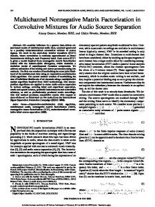
Figure 1. Cross-validation error versus dimensionality of a reduced space for JAFFE16 data. For Sonar cross-validation errors are shown in Fig. 2. Error rates for all methods in Rn were approximately identical and equal to 17.5% in ‘aspect-angle independent’ experiments9 . They were, however, worse (but not always) in Rr . Unlike JAFFE16, it is hard to say here when NMF could be used and for what classifier. 10−fold cross validation error vs. dimensionality 40 KNN KernelNN HKNN SVM NMF+KNN NMF+KernelNN NMF+HKNN NMF+SVM
35
4.3 Classification
30
25 Error rate (%)
In all experiments, 10-fold cross-validation was used in order to compute error rates. Let us assume the dimensionality of the original space is n, whereas that of the space obtained after dimensionality reduction is r with r < n. Cross-validation errors for each value of r are collected in groups of eight bars in figures below. The first four bars are associated with KNN, KernelNN, HKNN, and SVM, respectively, while other bars correspond to these classifiers coupled with NMF. For JAFFE16 KNN and HKNN demonstrated the best performance in Rn , though SVM closely followed it. Cross-validation errors are provided in Fig. 1. It is seen that NMF is useful for KNN and HKNN (the accuracy was sometimes lower in Rr than in Rn ), but not for KernelNN and SVM. We also experimented by applying all the four classifiers without NMF to images of various resolution (32 × 32, 64 × 64, 128 × 128, and 256 × 256 pixels). It turned out that the resolution did not influence on error rate. That is, low resolution images (as low as 16 × 16 pixels)
50 75 100 Dimensionality of a reduced space
20
15
10
5
0
6
12 18 24 Dimensionality of a reduced space
30
Figure 2. Cross-validation error versus dimensionality of a reduced space for Sonar data.
As remarked in [10], Liver data are highly nonlinear 9 This
result closely resembles results obtained by other researchers on this dataset.
Sammon stress vs. dimensionality 0.88
0.86
0.84 Sammon stress
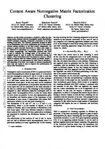
and hard to classify: accuracies achieved in [10] with KernelNN (K = 3, p = 3) and SVM (p = 3) are 71% and 68%, respectively. Thus, this set provides a challenge for classifiers and this is why we selected this dataset despite its low dimensionality. As with two previous examples, cross-validation errors are shown in Fig. 3. Again you can see that the accuracy degraded after dimensionality reduction, but not always dramatically. In fact, the accuracy of ‘NMF+classifier’ mostly lagged behind the results reported in [10].
Figure 4. Sammon-like stress versus dimensionality of a reduced space for JAFFE16 data.
30
Sammon stress vs. dimensionality
20
0.6 0.58
10
0.56
2
3 4 Dimensionality of a reduced space
5
Figure 3. Cross-validation error versus dimensionality of a reduced space for Liver data.
0.54 Sammon stress
0
0.52 0.5 0.48 0.46
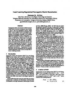
4.4 Topology Preservation In addition to classification error rates we computed a Sammon-like stress [12], E, in (8) measuring topology preservation of the original set after dimensionality reduction. Measurements were done for each dataset for different r’s and results are shown in Figs. 4-6. 1 E = Pm−1 Pm i=1
m−1 X
j=i+1 δij i=1
m X (δij − dij )2 , (8) δij j=i+1
where E ∈ [0, 1] with 0 indicating a lossless mapping Rn 7−→ Rr i.e. the closer E to zero, the better topology of the original space is preserved in a reduced space; dij and δij are the distances between the ith and jth points in Rn and Rr , respectively. All plots naturally indicate that topology is best preserved in higher dimensional than in lower dimensional spaces. However, there are distinctions between datasets. For example, when the dimensionality is reduced by half, the smallest E (≈ 0.23 for r = 3) was attained for Liver data whereas the largest E (slightly over 0.76 for r = 125) for JAFFE16 data. For Sonar data E ≈ 0.44 for r = 30. It
0.44
6
12 18 24 Dimensionality of a reduced space
30
Figure 5. Sammon-like stress versus dimensionality of a reduced space for Sonar data.
means that if one reduces the dimensionality by half by using NMF, the topology is best preserved for Liver data, followed by Sonar and JAFFE16 data. In other words, Liver data allow higher dimensionality reduction than the other two sets. Additional information about acceptable levels for dimensionality reduction can be learned from error rates associated with certain r’s for each classifier individually. Perhaps, a relative decrease of E is more important than its absolute value.
5 Discussion and Conclusion NMF coupled with four classifiers was tested on three realworld datasets with the aim to figure out when it will be
[2] S. Tsuge, M. Shishibori, S. Kuroiwa, & K. Kita, Dimensionality reduction using non-negative matrix factorization for information retrieval, Proc. 2001 IEEE Int. Conf. on Systems, Man, and Cybernetics, Tucson, AZ, 2001, 960-965.
Sammon stress vs. dimensionality 0.32 0.3
Sammon stress
0.28
[3] D. Guillamet, & J. Vitri`a, Discriminant basis for object classification, Proc. 11th Int. Conf. on Image Analysis and Processing, Palermo, Italy, 2001, 256261.
0.26 0.24 0.22
[4] D. Guillamet, & J. Vitri`a, Evaluation of distance metrics for recognition based on non-negative matrix factorization, Pattern Recognition Letters, 24(9-10), 2003, 1599-1605.
0.2 0.18 0.16 2
3 4 Dimensionality of a reduced space
5
Figure 6. Sammon-like stress versus dimensionality of a reduced space for Liver data.
useful. It turned out to be almost useless, except for classifying JAFFE16 data in Rr with KNN and especially with HKNN10 . The reason of this failure can be that NMF is designed to learn parts from objects. Only JAFFE16 is composed of objects - faces, while other two sets just contain numerical features which cannot be considered as “real objects” when combined together. That is, NMF can provide any valuable results only if a dataset includes images of physical objects/subjects, such as those of people, cars, etc. However, the standard NMF, though being claimed to learn parts, in fact, can be holistic, i.e. parts of objects learned by NMF are not necessarily always localized. Local NMF (LNMF) [6, 8] and Weighted NMF (WNMF) [5] both try to remedy this problem and therefore are worthy for consideration instead of NMF. Another deficiency of NMF lowering its practical value is that the standard NMF often produces correlated basis functions, i.e. despite dimensionality reduction the curse of dimensionality may be not totally avoided. In this case, correlated features can still deteriorate the performance of a classifier. It could be an explanation why NMF did not show clear advantages over PCA (it sometimes even lose to PCA) when classifying MNIST characters [4], Corel images [5], and ORL face images [6]. However, further research involving more datasets is definitely necessary before drawing stronger conclusions.
References [1] D.D. Lee, & H.S. Seung, Learning the parts of objects by non-negative matrix facorization, Nature, 401(6755), 1999, 788-791. 10 In fact, HKNN demonstrated an excellent performance in both original and reduced spaces and can be considered as a strong alternative to SVM.
[5] D. Guillamet, J. Vitri`a & B. Schiele, Introducing a weighted non-negative matrix factorization for image classification, Pattern Recognition Letters, 24(14), 2003, 2447-2454. [6] S.Z. Li, X.W. Hou, H.J. Zhang, & Q.S. Cheng, Learning spatially localized, parts-based representation, Proc. 2001 IEEE Conf. on Computer Vision and Pattern Recognition, Kauai, HW, 2001, 207-212. [7] B. Xu, J. Lu, & G. Huang, A constrained non-negative matrix factorization in information retrieval, Proc. 2003 IEEE Int. Conf. on Information Reuse and Integration, Las Vegas, NV, 2003, 273-277. [8] Y. Wang, Y. Jia, C. Hu, & M. Turk, Fisher nonnegative matrix factorization for learning local features, Proc. 6th Asian Conf. on Computer Vision, Jeju Island, Korea, 2004. [9] V. Vapnik, The nature of statistical learning theory (Berlin: Springer-Verlag, 1995). [10] K. Yu, L. Ji, & X. Zhang, Kernel nearest-neighbor algorithm, Neural Processing Letters, 15(2), 2002, 147156. [11] P. Vincent, & Y. Bengio, K-local hyperplane and convex distance nearest neighbor algorithms, in T.G. Dietterich, S. Becker, & Z. Ghahramani (Ed.) Advances in Neural Information Processing Systems, 14, (Cambridge, MA: MIT Press, 2002) 985-992. [12] E. Pe¸kalska, D. de Ridder, R.P.W. Duin, & M.A. Kraaijveld, A new method of generalizing Sammon mapping with application to algorithm speedup, Proc. 5th Annual Conf. of the Advanced School for Computing and Imaging, Heijen, the Netherlands, 1999, 221-228.