Non-Negative Matrix Factorization, Convexity and Isometry

Non-Negative Matrix Factorization, Convexity and Isometry Nikolaos Vasiloglou

Alexander G. Gray

arXiv:0810.2311v2 [cs.AI] 22 Apr 2009

Abstract In this paper we explore avenues for improving the reliability of dimensionality reduction methods such as Non-Negative Matrix Factorization (NMF) as interpretive exploratory data analysis tools. We first explore the difficulties of the optimization problem underlying NMF, showing for the first time that non-trivial NMF solutions always exist and that the optimization problem is actually convex, by using the theory of Completely Positive Factorization. We subsequently explore four novel approaches to finding globallyoptimal NMF solutions using various ideas from convex optimization. We then develop a new method, isometric NMF (isoNMF), which preserves non-negativity while also providing an isometric embedding, simultaneously achieving two properties which are helpful for interpretation. Though it results in a more difficult optimization problem, we show experimentally that the resulting method is scalable and even achieves more compact spectra than standard NMF.

1

Introduction.

In this paper we explore avenues for improving the reliability of dimensionality reduction methods such as NonNegative Matrix Factorization (NMF) [21] as interpretive exploratory data analysis tools, to make them reliable enough for, say, making scientific conclusions from astronomical data. NMF is a dimensionality reduction method of much recent interest which can, for some common kinds of data, sometimes yield results which are more meaningful than those returned by the classical method of Principal Component Analysis (PCA), for example (though it will not in general yield better dimensionality reduction than PCA, as we’ll illustrate later). For data of significant interest such as images (pixel intensities) or text (presence/absence of words) or astronomical spectra (magnitude in various frequencies), where the data values are non-negative, NMF can produce components which can themselves be interpreted as objects of the same type as the data which are added together to produce the observed data. In other words, the components are more likely to be sensible images or documents or spectra. This makes it a potentially very useful inter∗ Supported † Georgia

by Google Grants Institute of Technology

∗

David V. Anderson†

pretive data mining tool for such data. A second important interpretive usage of dimensionality reduction methods is the plot of the data points in the low-dimensional space obtained (2-D or 3-D, generally). Multidimensional scaling methods and recent nonlinear manifold learning methods focus on this usage, typically enforcing that the distances between the points in the original high-dimensional space are preserved in the low-dimensional space (isometry constraints). Then, apparent relationships in the low-D plot (indicating for example cluster structure or outliers) correspond to actual relationships. A plot of the points using components found by standard NMF methods will in general produce misleading results in this regard, as existing methods do not enforce such a constraint. Another major reason that NMF might not yield reliable interpretive results is that current optimization methods [18, 22] might not find the actual optimum, leading to poor performance in terms of both of the above interpretive usages. This is because its objective function is not convex, and so unconstrained optimizers are used. Thus, obtaining a reliably interpretable NMF method requires understanding its optimization problem more deeply – especially if we are going to actually create an additionally difficult optimization problem by adding isometry constraints. 1.1 Paper Organization. In Section 2 we first study at a fundamental level the optimization problem of standard NMF. We relate for the first time the NMF problem to the theory of Completely Positive Factorization, then using that theory, we show that every nonnegative matrix has a non-trivial exact non-negative matrix factorization of the form W=VH, a basic fact which had not been shown until now. Using this theory we also show that a convex formulation of the NMF optimization problem exists, though a practical solution method for this formulation does not yet exist. We then explore four novel formulations of the NMF optimization problem toward achieving a global optimum: convex relaxation using the positive semidefinite cone, approximating the semidefinite cone with smaller ones, convex multi-objective optimization, and generalized geometric programming. We highlight the difficul-

ties encountered by each approach. In order to turn to the question of how to create a new isometric NMF, in Section 3 we give background on two recent successful manifold learning methods, Maximum Variance Unfolding (MVU) [33] and a new variant of it, Maximum Furthest Neighbor Unfolding (MFNU) [25]. It has been shown experimentally [34] that they can recover the intrinsic dimension of a dataset very reliably and effectively, compared to previous well-known methods such as ISOMAP [31], Laplacian Eigen-Maps [2] and Diffusion Maps [6]. In synthetic experiments the above methods manage to decompose data into meaningful dimensions. For example, for a dataset consisting of images of a statue photographed from different horizontal and vertical angles, MVU and MFNU find two dimensions that can be identified as the horizontal and the vertical camera angle. MVU and MFNU contain ideas, particularly concerning the formulation of their optimization problems, upon which isometric NMF will be based. In Section 4 we show a practical algorithm for an isometric NMF (isoNMF for short), representing a new data mining method capable of producing both interpretable components and interpretable plots simultaneously. We use ideas for efficient optimization and efficient neighborhood computation to obtain a practical scalable method. In Section 5 we demonstrate the utility of isoNMF in experiments with datasets used in previous papers. We show that the components it finds are comparable to those found by standard NMF, while it additionally preserves distances much better, and also results in more compact spectra. 2

Convexity in Factorization.

Non

Negative

Matrix

×m Given a non-negative matrix V ∈ ℜN the goal of + ×k NMF is to decompose it in two matrices W ∈ ℜN , + k×m H ∈ ℜ+ such that V = W H. Such a factorization always exists for k ≥ m. The factorization has a trivial solution where W = V and H = Im . Determining the minimum k is a difficult problem and no algorithm exists for finding it. In general we can show that NMF can be cast as a Completely Positive (CP) Factorization problem [3]. ×N Definition 2.1. A matrix A ∈ ℜN is Completely + Positive if it can be factored in the form A = BB T , ×k where B ∈ ℜN . The minimum k for which A = BB T + holds is called the CP rank of A.

Not all matrices admit a completely positive factorization even if they are positive definite and non-negative. Notice though that for every positive definite non-

negative matrix a Cholesky factorization always exists, but there is no guarantee that the Cholesky factors are non-negative too. Up to now there is no algorithm of polynomial complexity that can decide if a given positive matrix is CP. A simple observation can show that A has to be positive definite, but this is a necessary and not a sufficient condition. ×N Theorem 2.1. If A ∈ ℜN is CP then rank(A) ≤ + N (N +1) − 1 cp-rank(A) ≤ 2

The proof can be found in [3]p.156. It is also conjectured 2 that the upper bound can be tighter N4 . ×N Theorem 2.2. if A ∈ ℜN is diagonally dominant1 , + then it is also CP.

The proof of the theorem can be found in [17]. Although CP factorization (A = BB T ) doesn’t exist for every matrix, we prove that non-trivial NMF (A = W H) always exists. ×m Theorem 2.3. Every non-negative matrix V ∈ ℜN + has a non-trivial, non-negative factorization of the form V = W H.

Proof. Consider the following matrix:   D V Z= (2.1) VT E ×k We want to prove that there always exists B ∈ ℜN + such that Z = BB T . If this is true then B can take the form:   W B= (2.2) HT

Notice that if D and E are arbitrary diagonally dominant completely positive matrices, then B always exists. The simplest choice would be to chose them as diagonal matrices where each element is greater or equal to the sum of rows/columns of V. Since they are diagonally dominant according to 2.2 Z is always CP. Since Z is CP then B exists so do W and H.  Although theorem 2.2 also provides an algorithm for constructing the CP-factorization, the cp-rank is usually high. A corollary of theorems 2.1 (cp-rank(A) ≥ rank(A)) and 2.3 (existence of NMF) is that SVD has always a more compact spectrum than NMF. There is no algorithm known yet for computing an exact NMF despite its existence. In practice, scientists try to minimize the norm [12, 22] of the factorization error. (2.3) min ||V − W H||2 W,H

1A

matrix is diagonally dominant if aii ≥

P

j6=i

|ai j|

This is the objective function we use in the experiments for this paper.

2.2 Convex relaxations of the NMF problem. In the following subsections we investigate convex relaxations of the NMF problem with the Positive Semidefi2.1 Solving the optimization problem of NMF. nite Cone [26]. Although in the current literature it is widely believed that NMF is a non-convex problem and only local min- 2.2.1 A simple convex upper bound with Sinima can be found, we will show in the following subsec- gular Value Decomposition. Singular Value Decomtions that a convex formulation does exist. Despite the position (SVD) can decompose a matrix in two factors existence of the convex formulation, we also show that U, V : a formulation of the problem as a generalized geomet- (2.9) A = UV ric program, which is non-convex, could give a better Unfortunately the sign of the SVD components of A ≥ 0 approach for finding the global optimum. cannot be guaranteed to be non-negative except for the first eigenvector [24]. However if we project U, V on 2.1.1 NMF as a convex conic program. the nonnegative orthant (U, V ≥ 0) we get a very good estimate (upper bound) for NMF. We will call it clipped Theorem 2.4. The set of Completely Positive MatriSVD, (CSVD). CSVD was used as a benchmark for the ces KCP is a convex cone. relaxations that follow. It has also been used as an initializer for NMF algorithms [20]. Proof. See [3]p.71. 2.2.2 Relaxation with a positive semidefinite cone. In the minimization problem of eq. 2.2.2 where the cost function is the L2 norm, the nonlinear terms wil hlj appear. A typical way to get these terms [26] would be to generate a large vector z = [W ′ (:); H(: )], where we use the MATLAB notation (H(:) is the   W V column-wise unfolding of a matrix). If Z = zz T min rank (2.4) T V H W,H (rank(Z) = 1) and z > 0 is true, then the terms appearing in ||V − W H||2 are linear in Z. In the subject to: following example eq. 2.10, 2.11 (see next page) where CP W∈K V ∈ ℜ2×3 , W ∈ ℜ2×2 , H ∈ ℜ2×3 we show the structure H ∈ KCP of Z. Terms in bold are the ones we need to express the (2.5) constraint V = W H, i.e v11 = w11 h11 + w12 h21 .   w11 Since minimizing the rank is non-convex, we can use its  w12  convex envelope that according to [28] is the trace of the    w21  matrix. So a convex relaxation of the above problem is:    w22       h11  W V   z= (2.10) (2.6) min Trace( )  VT H  h21  W,H  h12    (2.7) subject to:  h22    W ∈ KCP  h13  h23 H ∈ KCP It is always desirable to find the minimum rank of NMF since we are looking for the most compact representation of the data matrix V . Finding the minimum rank NMF can be cast as the following optimization problem:

(2.8)

Now the optimization problem eq. is equivalent to:

i=N,j=m k After determining W, H, W and H can be recovered X X 2 (Zik+l,N k+jk+l − Vij ) by CP factorization of W, H, which again is not an (2.12) min i=1,j=1 l=1 easy problem. In fact there is no practical barrier function known yet for the CP cone so that Interior subject to: Point Methods can be employed. Finding a practical rank(Z) = 1 description of the CP cone is an open problem. So although the problem is convex, there is no algorithm This is not a convex problem but it can be easily known for solving it. be relaxed to [7]:

2

6 6 6 6 6 6 6 (2.11) Z = 6 6 6 6 6 6 6 4

(2.13)

2 w11 w12 w11 w21 w11 w22 w11 h11 w11 h21 w11 h12 w11 h22 w11 h13 w11 h23 w11

w11 w12 2 w12 w21 w12 w22 w12 h11 w12 h21 w12 h12 w12 h22 w12 h13 w12 h23 w12

w11 w21 w12 w21 2 w21 w22 w21 h11 w21 h21 w21 h12 w21 h22 w21 h13 w21 h23 w21

w11 w22 w12 w22 w21 w22 2 w22 h11 w22 h21 w22 h12 w22 h22 w22 h13 w22 h23 w22

w11 h11 w12 h11 w21 h11 w22 h11 h211 h21 h11 h12 h11 h22 h11 h13 h11 h23 h11

min Trace(Z) subject to: A•Z Z Z Z

= Vij  0  zz T ≥ 0

where A is a matrix that selects the appropriate elements from Z. Here is an example for a matrix A that selects the elements of Z that should sum to the V13 element:   0 0 0 0 1 0    0 0 0 0 0 0 1   0 0 0 0 0 0  (2.14) A13 =    0 0 0 0 0 0  0 0

In the second formulation (2.13) we have relaxed Z = zz T with Z  zz T . The objective function tries to minimize the rank of the matrix, while the constraints try to match the values of the given matrix V . After solving the optimization problem the solution can be found on the first eigenvector of Z. The quality of the relaxation depends on the ratio of the first eigenvalue to sum of the rest. The positivity of Z will guarantee that the first eigenvector will have elements with the same sign according to the Peron Frobenious Theorem [24]. Ideally if the rest of the eigenvectors are positive they can also be included. One of the problems of this method is the complexity. Z is (N +m)k×(N +m)k and +m)k−1) non-negative constraints. there are ((N +m)k)((N 2 Very quickly the problem becomes unsolvable. In practice the problem as posed in 2.12 always gives W and H matrices that are rank one. After testing the method exhaustively with random matrices V that either had a product V = W H representation or not the solution was always rank one on both W and H. This was always the case with any of the convex formulations presented in this paper. This is because there is a

w11 h21 w12 h21 w21 h21 w22 h21 h11 h21 h221 h12 h21 h22 h21 h13 h21 h23 h21

w11 h12 w12 h12 w21 h12 w22 h12 h11 h12 h21 h12 h212 h22 h12 h13 h12 h23 h12

w11 h22 w12 h22 w21 h22 w22 h22 h11 h22 h21 h22 h12 h22 h222 h13 h22 h23 h22

w11 h13 w12 h13 w21 h13 w22 h13 h11 h13 h21 h13 h12 h13 h22 h13 h213 h23 h13

w11 h23 w12 h23 w21 h23 w22 h23 h11 h23 h21 h23 h12 h23 h22 h23 h13 h23 h223

3 7 7 7 7 7 7 7 7 7 7 7 7 7 7 5

missing constraint that will let the energy of the dot products spread among dimensions. This is something that should characterize the spectrum of H. The H matrix is often interpreted as the basis vectors of the factorization and W as the matrix that has the coefficients. It is widely known that in nature spectral analysis is giving spectrum that decays either exponentially e−λf or more slowly 1/f γ . Depending on the problem we can try different spectral functions. In our experiments we chose the exponential one. Of course the decay parameter λ is something that should be set adhoc. We experimented with several values of λ, but we couldn’t come up with a systematic, heuristic and practical rule. In some cases the reconstruction error was low but in some others not. Another relaxation that was necessary for making the optimization tractable was to reduce the the non-negativity constraints only on the elements that are involved in the equality constraints. 2.2.3 Approximating the SDP cone with smaller ones. A different way to deal with the computational complexity of SDP (eq. 2.13) is to approximate the big SDP cone (N + m)k × (N + m)k with smaller ones. Let Wi be the ith row of W and Hj the jth column of H. Now zij = [Wi (:)′ ; Hj (:)] (2k dimensional vector) T and Zij = zij zij (2k × 2k matrix), or   WiT Wi WiT Hj Zij = (2.15) WiT Hj Hj HjT or it is better to think it in the form:   Wi ZW H (2.16) Zij = ZW H Hj and once W, H are found then Wi , Hj can be found from SVD decomposition of W, H and the quality of the relaxation will be judged upon the magnitude of the first eigenvalue compared to the sum of the others. Now the optimization problem becomes: (2.17)

min

N X m X i=1 j=1

Trace(Zij )

Zij Zij

≥ 

0 0

Aij • Zij

=

vij ,

An immediate consequence is that ∀i, j

(2.21)

til

≥ Wil2

(2.22) tjl ≥ Hll2 2 2 2 The above method has N m constraints. In terms of (2.23)(til − Wil )(tjl − Hlj ) ≥ (Vij,l − Wil Hlj ) storage it needs In above that the L2 error PNthePm Pk inequality we see 2 (V − W H ) becomes zeros if til = • (N + m) symmetric positive definite k × k maij,l il lj i=1 j=1 l=1 trices for every row/column of W, H, which is Wil2 , tjl = Hil2 , ∀til , tjl . In general we want to min(N +m)k(k+1) imize t while maximizing ||W ||2 and ||H||2 . L2 norm 2 maximization is not convex, but instead we can max• N m symmetric positive definite k × k matrices for imize P W , P H which are equal to the L norms il lj 1 every Wi Hj product, which is (N m)k(k+1) since everything is positive. This can be cast as convex 2 2 In total the storage complexity is O((N + m + multi-objective problem on the second order cone [4]. " # Pi=N Pk P Pk ) which is significantly smaller by an order N m) k(k+1) 2 til + j=m tlj i=1 l=1 j=1 l=1 +m)k−1) Pi=N Pk Pj=m Pk min of magnitude from O( (N +m)k((N ) which is the 2 − i=1 j=1 l=1 Wil − l=1 Hlj complexity of the previous method. There is also sigsubject to : nificant improvement in the computational part. The (2.24)   til − Wil2 Vij,l − Wil Hlj SDP problem is solved with interior point methods [26] 0 Vij,l − Wil Hlj tjl − Hlj2 that require the inversion of a symmetric positive definite matrix at some point. In the previous method that would require O((N + m)3 k 3 ) steps, while with Unfortunately multi-objective optimization problems, this method we have to invert N m 2k × 2k matrices, even when they are convex, they have local minima that that would cost N m(2k)3 . Because of their special are not global. An interesting direction would be to test structure the actual cost is (N m)k 3 + max(N, m)k 3 = the robustness of existing multi-objective algorithms on NMF. (N m + max(N, m))k 3 . We know that Wi , Hj  0. Since Zij is PSD and 2.2.5 Local solution of the non-convex problem. according to Schur’s complement on eq. 2.16: In the previous sections we gave several convex formu−1 lations and relaxations of the NMF problem that unfor(2.18) Hj − ZW H Wi ZW H  0 tunately are either unsolvable or they give trivial rank So instead of inverting (2.16) that would cost 8k 3 we one solutions that are not useful at all. can invert 2.18. This formulation gives similar results In practice the non-convex formulation of eq. 2.2.2 with the big SDP cone and most of the cases the results (classic NMF objective) along with other like the KL are comparable to the CSVD. distance between V and W H are used in practice [22]. All of them are non-convex and several methods have 2.2.4 NMF as a convex multi-objective prob- been recommended, such as alternating least squares, lem. A different approach would be to find a convex gradient decent or active set methods [18]. In our set in which the solution of the NMF lives and search experiments we used the L-BFGS method that scales for it over there. Pm Assume that we want to match very well for large matrices. Vij = Wi Hj = l=1 Wil Hlj . In this section we show that by controlling the ratio of the L2 /L1 norms of 2.2.6 NMF as a Generalized Geometric ProW, H it is possible to find Pk the solution to NMF. De- gram and it’s Global Optimum. The objective fine Wil Hlj = Vij,l and l=1 Vij,l = Vij . We form the function (eq. 2.2.2) can be written in the following form: following matrix that we require to be PSD: N X m X k X   2 (2.25) ||V − W H|| = (Vij − Wil Hlj ) 2 1 Wil Hlj i=1 j=1 l=1  Wil til Vij,l   0 (2.19) Hlj Vij,l tjl The above function is twice differentiable so according

If we use the Schur complement we have:   Vij,l − Wil Hlj til − Wil2 (2.20) 0 Vij,l − Wil Hlj tjl − Hlj2

to [11] the function can be cast as the difference of convex (d.c.) functions. The problem can be 2 also

known as vector optimization

solved with general off-the-shelf global optimization algorithms. It can also be formulated as a special case of dc programming, the generalized geometric programming. With the following transformation Wil = ˜ ew˜il , Hlj = ehlj the objective becomes: N X m X k  2 X ˜ Vij − ew˜il +hlj

(2.26) ||V − W H||2 =

i=1 j=1 l=1

=

m N X X

Vij2

+

i=1 j=1

i=1 j=1

−2

N X m X

k m N X X X k X

Vij

i=1 j=1

e

e

˜ lj w ˜il +h

l=1

˜ lj w ˜il +h

l=1

!2

!

The first term is constant and it can be ignored for the optimization. The other two terms: ˜ lj ) = (2.27)f (w ˜il , h

N X m X i=1 j=1

˜ lj ) = (2.28) g(w ˜il , h

2

N X m X i=1 j=1

k X

˜

ew˜il +hlj

l=1

Vij

k X l=1

e

!2

˜ lj w ˜il +h

!

are convex functions also known as the exponential form of posynomials 3 [4]. For the global solution of the problem ˜ , H) ˜ − g(W ˜ , H) ˜ (2.29) min f (W ˜ ,H ˜ W

the algorithm proposed in [8] can be employed. The above algorithm uses a branch and bound scheme that is impractical for high dimensional optimization problems as it requires too many iterations to converge. It is worthwhile though to compare it with thelocal nonconvex NMF solver on a small matrix. We tried to do NMF of order 2 on the following random matrix:   0.45 0.434 0.35  0.70 0.64 0.43  0.22 0.01 0.3

After 10000 restarts of the local solver the best error we got was 2.7% while the global optimizer very quickly gave 0.015% error, which is 2 orders of magnitude less than the local optimizer. Another direction that is not investigated in this paper is the recently developed algorithm for Difference Convex problems by Tao [30] that has been applied successfully to other data mining applications such as Multidimensional Scaling. [1]. 3 Posynomial is a product of positive variables exponentiated in any real number

3 Isometric Embedding The key concept in Manifold Learning (ML)is to represent a dataset in a lower dimensional space by preserving the local distances. The differences between methods Isomap [31], Maximum Variance unfolding (MVU) [33], Laplacian EigenMaps [2] and Diffusion Maps [6] is how they treat distances between points that are not in the local neighborhood. For example IsoMap preserves exactly the geodesic distances, while Diffusion Maps preserves distances that are based on the diffusion kernel. Maximum Furthest Neighbor Unfolding (MFNU) [25] that is a variant of Maximum Variance Unfolding, preserves local distance and it tries to maximize the distance between furthest neighbors. In this section we are going to present the MFNU method as it will be the basis for building isoNMF. 3.1 Convex Maximum Furthest Neighbor Unfolding. Weinberger formulated the problem of isometric unfolding as a Semidefinite Programming algorithm [33]4 . In [19] Kulis presented a non-convex formulation of the problem that requires less memory than the Semidefinite one. He also claimed that the non-convex formulation is scalable. The non-convex formulation has the same global optimum with the Semidefinite one as proven in [5]. In [25] Vasiloglou presented experiments where he verified the scalability of this formulation. A variant of MVU the Maximum Furthest Neighbor Unfolding (MFNU) was also presented in the same paper. The latest formulation tends to be more robust and scalable than MVU, this is why we will employ it as the basis of isoNMF. Both methods can be cast as a semidefinite programming problem [32]. Given a set of data X ∈ ℜN ×d , where N is the number of points and d is the dimensionality, the dot product or Gram matrix is defined as G = XX T . The goal is to find a new Gram matrix K such that ˆX ˆT rank(K) < rank(G) in other words K = X N ×d′ ′ ˆ where X ∈ ℜ and d < d. Now the dataset ˆ which has fewer dimensions than is represented by X X. The requirement of isometric unfolding is that the ′ euclidian distances in the ℜd for a given neighborhood around every point have to be the same as in the ℜd . This is expressed in: Kii + Kjj − Kij − Kji = Gii + Gjj − Gij − Gji , ∀i, j ∈ Ii where Ii is the set of the indices of the neighbors of the ith point. From all the K matrices MFNU chooses the one that maximizes the distances between furthest

4A

similar approach to learning metrics is given in [29]

neighbor pairs. So the algorithm is presented as an SDP: max K

N X

−

λij (Aij • RRT − di j)

i=1 ∀j∈Ii

Bi • K

i=1

+

subject to Aij • K K

N X X

= dij  0

∀j ∈ Ii

N σX X (Aij • RRT − dij )2 2 i=1 ∀j∈Ii

Our goal is to minimize the Lagrangian that’s why the objective function is −RRT and not RRT The derivative of the augmented Lagrangian is: where the A • X = Trace(AX T ) is the dot product between matrices. Aij has the following form: N X ∂L   (3.34) Bi • R = −2 1 0 . . . −1 . . . 0 ∂R i=1    0 ... 0 . . . 0 0  N X X    ..  . λij Aij R −2 .. 0 . . . 0   . 0 (3.30)   i=1 ∀j∈Ii  −1 . . . 0  1 ... 0   N X X  .   .. (Aij • RRT − di j)Aij R 2σ 0 ... 0 ... 0  i=1 ∀j∈Ii 0 ... ... 0 ... 0

and (3.31)

dij = Gii + Gjj − Gij − Gji

Gradient descent is a possible way to solve the minimization of the Lagrangian, but it is rather slow. The Newton method is also prohibitive. The Hessian of this problem is a sparse matrix although the cost of the inversion might be high it is worth investigating. In our experiments we used the limited memory BFGS (LBFGS) method [23, 27] that is known to give a good rate for convergence. MFNU in this non-convex formulation behaves much better than MVU. In the experiments presented in [25], MFNU tends to find more often the global optimum, than MVU. The experiments also showed that the method scales well up to 100K points.

Bi has the same structure of Aij and computes the distance of the ith point with its furthest neighbor. The last condition is just a centering constraint for ˆ are the covariance matrix. The new dimensions X the eigenvectors of K. In general MFNU gives Gram matrices that have compact spectrum, at least more compact than traditional linear Principal Component Analysis (PCA). The method behaves equally well with MVU. Both MVU and MFNU are convex so they converge to the global optimum. Unfortunately this method can handle datasets of no more than hundreds of points because of its complexity. In the following 4 Isometric NMF. section a non-convex formulation of the problem that NMF and MFNU are optimization problems. The goal of isoNMF is to combine these optimization problems scales better is presented. in one optimization problem. MFNU has a convex and 3.2 The Non Convex Maximum Furthest a non-convex formulation, while for NMF only a nonNeighbor Unfolding. By replacing the constraint convex formulation that can be solved is known. K  0 [5] with an explicit rank constraint K = RRT the problem becomes non-convex and it is reformulated 4.1 Convex isoNMF. By using the theory presented in section 2.1.1 we can cast isoNMF as a convex to problem: N X T (3.32) max Bi • RR N X i=1 (4.35) Bi • Z max ˜ ,H ˜ W subject to: i=1 subject to: Aij • RRT = dij ˜ = dij Aij • W In [5], Burer proved that the above formulation has the   ˜ W V same global minimum with the convex one. Z= ˜ The above problem can be solved with the augVT H mented Lagrangian method [27]. Z ∈ KCP (3.33) L =

−

N X i=1

Bi • RRT

˜ ∈ KCP W ˜ ∈ KCP H

Then W, H can be found by the completely positive ˜ = WWT,H ˜ = HH T . Again this factorization of W problem although it is convex, there is no polynomial algorithm known for solving it. 4.2 Non-convex formulation of isoNMF. The non convex isoNMF can be cast as the following problem: (4.36)

N X

max

Bi • W W T

i=1

subject to: Aij • W W T = dij WH = V W ≥0 H≥0 The augmented lagrangian with quadratic penalty function is the following: (4.37) L

= −

N X

Bi • W W T

i=1

−

N X X

λij (Aij • W W T − di j)

i=1 ∀j∈Ii

−

N X m X i=1 j=1

+

µij

k X

(Wik Hkj − Vij )

l=1

N σ1 X X (Aij • W W T − dij )2 2 i=1 ∀j∈Ii

+

σ2 2

N X m X k X i=1 j=1 l=1

(Wil Hlj − Vij )2

+2σ2

N X m X k X

(Wil Hlj − Vij )H

i=1 j=1 l=1

(4.39)

N X m X ∂L µij H =− ∂H i=1 j=1

+2σ2

N X m X k X

(Wil Hlj − Vij )W

i=1 j=1 l=1

4.3 Computing the local neighborhoods. As already discussed in previous section MFNU and isoNMF require the computation of all-nearest and all-furthest neighbors. The all-nearest neighbor problem is a special case of a more general class of problems called N-body problems [10]. In the following sections we give a sort description of the nearest neighbor computation. The actual algorithm is a four-way recursion. More details can be found in [10]. 4.3.1 Kd-tree. The kd-tree is a hierarchical partitioning structure for fast nearest neighbor search [9]. Every node is recursively partitioned in two nodes until the points contained are less than a fixed number. This is a leaf. Nearest neighbor search is based on a top down recursion until the query point finds the closest leaf. When the recursion hits a leaf then it searches locally for a candidate nearest neighbor. At this point we have an upper bound for the nearest neighbor distance, meaning that the true neighbor will be at most as far away as the candidate one. As the recursion backtracks it eliminates (prunes) nodes that there are further away than the candidate neighbor. Kd-trees provide on the average nearest neighbor search in O(log N ) time, although for pathological cases the kd-tree performance can asymptotically have linear complexity like the naive method.

The non-negativity constraints are missing from the Lagrangian. This is because we can enforce them through the limited bound BFGS also known as L- 4.3.2 The Dual Tree Algorithm for nearest BFGS-B. The derivative of the augmented Lagrangian neighbor computation. In the single tree algorithm is: the reference points are ordered on a kd-tree. Every nearest neighbor computation requires O(log(N )) comN X ∂L putations. Since there are N query points the total (4.38) Bi W = −2 ∂W cost is O(N log(N )). The dual-tree algorithm [10] ori=1 ders the query points on a tree too. If the query set N X X and the reference set are the same then they can share λij Aij W −2 the same tree. Instead of querying a single point at a i=1 ∀j∈Ii time the dual-tree algorithm always queries a group of N X m X points that live in the same node. So instead of doµij H − ing the top-down recursion individually for every point i=1 j=1 it does it for the whole group at once. Moreover inN X X T stead of computing distances between points and nodes (Aij • W W − di j)Aij W +2σ1 it computes distances between nodes. This is the reai=1 ∀j∈Ii

son why most of the times the dual-tree algorithm can prune larger portions of the tree than the single tree algorithm. The complexity of the dual-tree algorithm is empirically O(N ). If the dataset is pathological then the algorithm can be of quadratic complexity too. The pseudo-code for the algorithm is described in fig. 1. recurse(q : KdTree, r : KdTree) { if (max_nearest_neighbor_distance_in_node(q) < distance(q, r) { /* prune */ } else if (IsLeaf(q)==true and IsLeaf(r)==true) { /* search for every point in q node */ /* its nearest neighbor in the r node */ /* at leaves we must resort to */ /* exhaustive search O(n^2) */ /*update the maximum_neighbor_distance_in_node(q)*/ } else if (IsLeaf(q)==false and IsLeaf(r)=true { /* choose the child that is closer to r */ /* and recurse first */ recurse(closest(r, q.left, q.right), r) recurse(furthest(r, q.left, q.right), r) } else if (IsLeaf(q)==true and IsLeaf(r)==false) { /* choose the child that is closer to q */ /* and recurse first */ recurse(q, closest(q, r.left, r.right)) recurse(q, furthest(q, r.left, r.right)) } else { recurse(q.left,closest(q.left, r.left, r.right)); recurse(q.left,furthest(q.left, r.left, r.right)); recurse(q.right,closest(q.right, r.left, r.right)); recurse(q.right,furthest(q.right, r.left, r.right)); } }

Figure 1: Pseudo-code for the dual-tree all nearest neighbor algorithm

4.3.3 The Dual Tree Algorithm for all furthest neighbor algorithm. Computing the furthest neighbor with the naive computation is also of quadratic complexity. The use of trees can speed up the computations too. It turns out that furthest neighbor search for a single query point is very similar to the nearest neighbor search presented in the original paper of kd-tree [9]. The only difference is that in the top-down recursion the algorithm always chooses the furthest node. Similarly in the bottom up recursion we prune a node only if the maximum distance between the point and the node is smaller than the current furthest distance. The pseudo code is presented in fig. 2.

recurse(q : KdTree, r : KdTree) { if (min_furthest_neighbor_distance_in_node(q) < distance(q, r) { /* prune */ } else if (IsLeaf(q)==true and IsLeaf(r)==true) { /* search for every point in q node its /* furthest neighbor in the r node */ /* at leaves we must resort to */ /* exhaustive search O(n^2) */ /*update the minimum_furthest_distance_in_node(q)*/ } else if (IsLeaf(q)==false and IsLeaf(r)=true { /*choose the child that is furthest to r */ /* and recurse first */ recurse(furthest(r, q.left, q.right), r) recurse(closest(r, q.left, q.right), r) } else if (IsLeaf(q)==true and IsLeaf(r)==false) { /* choose the child that is furthest to q */ /* and recurse first */ recurse(q, furthest(q, r.left, r.right)) recurse(q, closest(q, r.left, r.right)) } else { recurse(q.left,furthest(q.left, r.left, r.right)); recurse(q.left,closest(q.left, r.left, r.right)); recurse(q.right,furthest(q.right, r.left, r.right)); recurse(q.right,closest(q.right, r.left, r.right)); } }

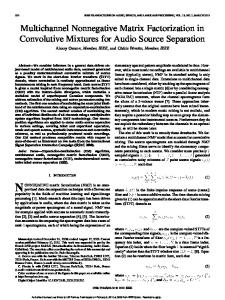
Figure 2: Pseudo-code for the dual-tree all furthest neighbor algorithm 1. The CBCL faces database fig. 3(a,b) [13], used in the experiments of the original paper on NMF [21]. It consists of 2429 grayscale 19 × 19 images that they are hand aligned. The dataset was normalized as in [21]. 2. The isomap statue dataset fig. 3(c) [14] consists of 698 64 × 64 synthetic face photographed from different angles. The data was downsampled to 32 × 32 with the Matlab imresize function (bicubic interpolation). 3. The ORL faces [15] fig. 3(d) presented in [12]. The set consists of 472 19 × 19 gray scale images that are not aligned. For visualization of the results we used the nmfpack code available on the web [16].

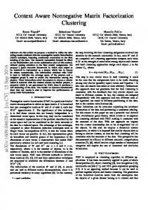
The results for classic NMF and isoNMF with kneighborhood equal to 3 are presented in fig. 4 and tables 1, 2. We observe that classic NMF gives always lower reconstruction error rates that are not that far away from the isoNMF. Classic NMF fails to preserve distances contrary to isoNMF that always does a good 5 Experimental Results job in preserving distances. Another observation is In order to evaluate and compare the performance of that isoNMF gives more sparse solution than classic isoNMF with traditional NMF we picked 3 benchmark NMF. The only case where NMF has a big difference datasets that have been tested in the literature: in reconstruction error is in the CBCL-face database

when it is being preprocessed. This is mainly because the preprocessing distorts the images and spoils the manifold structure. If we don’t do the preprocessing fig. 4(f), the reconstruction error of NMF and isoNMF are almost the same. We would also like to point that isoNMF scales equally well with the classic NMF. Moreover they are seem to show the same sensitivity to the initial conditions. In fig. 6 we see a comparison of the energy spectrums of classic NMF and isoNMF. We define the spectrum as PN 2 l=1 Wli si = qP M 2 l=1 Hil

classic NMF rec. error sparsity dist. error

cbcl norm. 22.01% 63.23% 92.10%

cbcl 9.20% 29.06% 98.61%

statue 13.62% 48.36% 97.30%

orl 8.46% 46.80% 90.79%

Table 1: Classic NMF, the relative root mean square error, sparsity and distance error for the four different datasets (cbcl normalized and plain, statue and orl) isoNMF rec error sparsity dist. error

cbcl norm. 33.34% 77.69% 4.19%

cbcl 10.16% 43.98% 3.07%

statue 16.81% 53.84% 0.03%

orl 11.77% 54.86% 0.01%

Table 2: isoNMF, the relative root mean square error, sparsity and distance error for the four different datasets This represents the energy of the component normalized (cbcl normalized and plain, statue and orl) by the energy of the prototype image generated by NMF/isoNMF. Although the results show that isoNMF 6 Conclusion is much more compact than NMF, it is not a reasonable metric. This is because the prototypes (rows of the In this paper we presented a deep study of the optimization problem of NMF, showing some fundamental H matrix Pk are not orthogonal PN Pm to each2 other. So in existence theorems for the first time as well as various reality i=1 si < i=1 j=1 (W H)ij and actually much smaller. This is because the dot product between advanced optimization approaches – convex and nonconvex, global and local. We believe that this study the rows is not zero. has the capability to open doors for further advances in NMF-like methods as well as other machine learning problems. We also developed and experimentally demonstrated a new method, isoNMF, which preserves both non-negativity and isometry, simultaneously providing two types of interpretability. With the added reliability and scalability stemming from an effective optimization algorithm, we believe that this method represents a potentially valuable practical new tool for the exploratory analysis of common data such as images, text, and spectra. (a) (b) References

(c)

(d)

Figure 3: (a)Some images from the cbcl face database (b)The same images after variance normalization, mean set to 0.25 and thresholding in the interval [0,1] (c)The synthetic statue dataset from the isomap website [14] (d)472 images from the orl faces database [15]

[1] L.T.H. An and P.D. Tao. DC Programming Approach and Solution Algorithm to the Multidimensional Scaling Problem. From Local to Global Optimization, pages 231–276, 2001. [2] M. Belkin and P. Niyogi. Laplacian Eigenmaps for Dimensionality Reduction and Data Representation, 2003. [3] A. Berman and N. Shaked-Monderer. Completely Positive Matrices. World Scientific, 2003. [4] S.P. Boyd and L. Vandenberghe. Convex Optimization. Cambridge University Press, 2004. [5] S. Burer and R.D.C. Monteiro. A nonlinear programming algorithm for solving semidefinite programs via low-rank factorization. Mathematical Programming, 95(2):329–357, 2003.

(a)

(b)

(c)

(d)

(e)

(f)

(g)

(h)

Figure 4: Top row: 49 Classic NMF prototype images. Bottom row: 49 isoNMF prototype images (a, e) CBCL-face database with mean variance normalization and thresholding, (b, f ) CBCL face database without preprocessing, (c, g) Statue dataset (d, h)ORL face database [6] R.R. Coifman and S. Lafon. Diffusion maps. Applied and Computational Harmonic Analysis, 21(1):5–30, 2006. [7] M. Fazel, H. Hindi, and SP Boyd. A rank minimization heuristic with application to minimum ordersystem approximation. American Control Conference, 2001. Proceedings of the 2001, 6, 2001. [8] C.A. Floudas. Deterministic Global Optimization: Theory, Methods and Applications. Kluwer Academic Pub, 2000. [9] J.H. Friedman, J.L. Bentley, and R.A. Finkel. An Algorithm for Finding Best Matches in Logarithmic Expected Time. ACM Transactions on Mathematical Software, 3(3):209–226, 1977. [10] A. Gray and A.W. Moore. N-Body problems in statistical learning. Advances in Neural Information Processing Systems, 13, 2001. [11] R. Horst and H. Tuy. Global Optimization: Deterministic Approaches. Springer, 1996. [12] P.O. Hoyer. Non-negative Matrix Factorization with Sparseness Constraints. The Journal of Machine Learning Research, 5:1457–1469, 2004. [13] http://cbcl.mit.edu/cbcl/softwaredatasets/FaceData2.html. [14] http://isomap.stanford.edu/face data.mat.Z. [15] http://www.cl.cam.ac.uk/research/dtg/ attarchive/facedatabase.html. [16] http://www.cs.helsinki.fi/u/phoyer/software.html. [17] M. Kaykobad. On nonnegative factorization of matrices. Linear Algebra and its Applications, 96:27–33, 1987.

[18] H. Kim and H. Park. Non-Negative Matrix Factorization Based on Alternating Non-Negativity Constrained Least Squares and Active Set Method. [19] B. Kulis, A.C. Surendran, and J.C. Platt. Fast LowRank Semidefinite Programming for Embedding and Clustering. In Eleventh International Conference on Artifical Intelligence and Statistics, AISTATS 2007, 2007. [20] A.N. Langville, C.D. Meyer, and R. Albright. Initializations for the nonnegative matrix factorization. Proc. of the 12 ACM SIGKDD International Conference on Knowledge Discovery and Data Mining, 2006. [21] D.D. Lee and H.S. Seung. Learning the parts of objects by non-negative matrix factorization. Nature, 401(6755):788–791, 1999. [22] D.D. Lee and H.S. Seung. Algorithms for Non-negative Matrix Factorization. ADVANCES IN NEURAL INFORMATION PROCESSING SYSTEMS, pages 556– 562, 2001. [23] D.C. Liu and J. Nocedal. On the limited memory BFGS method for large scale optimization. Mathematical Programming, 45(1):503–528, 1989. [24] H. Minc. Nonnegative matrices. Wiley New York, 1988. [25] D. Anderson N. Vasiloglou, A. Gray. Scalable Semidefnite Manifold Learning. IEEE Machine Learning in Signal Processing, 2008. [26] Nemirovski A. Lectures on Modern Convex Optimization. [27] J. Nocedal and S.J. Wright. Numerical Optimization. Springer, 1999.

normalized energy

0.8 0.6 0.4

1

1

0.8

0.8 normalized energy

1

0.6 0.4 0.2

0.2 0 0

(a)

(a) 0.2

0.4

0.6

0.8

0 0

0.6 0.4 0.2

10

20 30 NMF dimension

1

40

50

(b)

0 0

10

20 30 NMF dimension

40

1

1 normalized energy

0.8

0.8

0.6

0.6 0.4 0.2

0.4

(c)

0.2

(b)

0 0

0.2

0.4

0.6

0.8

1

1 0.8 0.6 0.4

0 0

10

20 30 NMF dimension

40

50

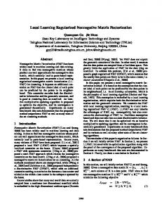
Figure 6: In this set of figures we show the spectrum of classic NMF (solid line) and Isometric NMF (dashed line) for the three datasets (a)cbcl face (b)isomap statue (c)orl faces. Although isoNMF gives much more compact spectrum we have to point that the basis functions are not orthogonal, so this figure is not comparable to SVD type spectrums

0.2

(c)

0 0

0.2

0.4

0.6

0.8

1

Figure 5: Scatter plots of two largest components of classic NMF(in blue) and Isometric NMF(in red) for (a)cbcl faces (b)isomap faces (c)orl faces

[28] B. Recht, M. Fazel, and P.A. Parrilo. Guaranteed Minimum-Rank Solutions of Linear Matrix Equations via Nuclear Norm Minimization. Arxiv preprint arXiv:0706.4138, 2007. [29] R. Rosales and G. Fung. Learning sparse metrics via linear programming. In Proceedings of the 12th ACM SIGKDD international conference on Knowledge discovery and data mining, pages 367–373. ACM New York, NY, USA, 2006. [30] P.D. Tao and L.T.H. An. Difference of convex functions optimization algorithms (DCA) for globally minimizing nonconvex quadratic forms on Euclidean balls and spheres. Operations Research Letters, 19(5):207– 216, 1996. [31] J.B. Tenenbaum, V. Silva, and J.C. Langford. A Global Geometric Framework for Nonlinear Dimensionality Reduction, 2000. [32] L. Vandenberghe and S. Boyd. Semidefinite Programming. SIAM Review, 38(1):49–95, 1996. [33] K.Q. Weinberger and L.K. Saul. An introduction

to nonlinear dimensionality reduction by maximum variance unfolding. Proceedings of the Twenty First National Conference on Artificial Intelligence (AAAI06), 2006. [34] K.Q. Weinberger, F. Sha, and L.K. Saul. Learning a kernel matrix for nonlinear dimensionality reduction. In Proceedings of the twenty-first international conference on Machine learning. ACM New York, NY, USA, 2004.

50