Non-Uniform Subset Selection for Active Learning in Structured Data

Non-Uniform Subset Selection for Active Learning in Structured Data Sujoy Paul, Jawadul H. Bappy and Amit Roy-Chowdhury Department of Electrical and Computer Engineering, University of California, Riverside, CA 92521 {supaul, mbappy, amitrc}@ece.ucr.edu

Abstract

labeling, without compromising recognition performance.

Several works have shown that relationships between data points (i.e., context) in structured data can be exploited to obtain better recognition performance. In this paper, we explore a different, but related, problem: how can these interrelationships be used to efficiently learn and continuously update a recognition model, with minimal human labeling effort. Towards this goal, we propose an active learning framework to select an optimal subset of data points for manual labeling by exploiting the relationships between them. We construct a graph from the unlabeled data to represent the underlying structure, such that each node represents a data point, and edges represent the inter-relationships between them. Thereafter, considering the flow of beliefs in this graph, we choose those samples for labeling which minimize the joint entropy of the nodes of the graph. This results in significant reduction in manual labeling effort without compromising recognition performance. Our method chooses non-uniform number of samples from each batch of streaming data depending on its information content. Also, the submodular property of our objective function makes it computationally efficient to optimize. The proposed framework is demonstrated in various applications, including document analysis, scene-object recognition, and activity recognition.

1. Introduction Over the years, due to advances in technology, huge amount of unlabeled visual and text data is generated daily. Also, machine learning algorithms are becoming more commonplace in human life. A large proportion of these algorithms are based on supervised learning which requires a large quantity of data to be labeled. Moreover, these models need to be updated over time as new data becomes available in order to dynamically adapt to the concepts of different classes which may drift with time. Manually labeling this continuous flow of data is not only a tedious task for humans but also prone to wrong labeling. Active Learning [39] can be a solution to this problem to reduce the amount of manual 3138

The ability of active learning to reduce manual labeling effort is due to the fact that not all training samples are valuable for building the recognition model [28]. Most active learning approaches formulate a utility score for each unlabeled sample, based on which they are chosen for manual labeling. Classifier uncertainty [31], information density [30], expected change in gradient [39], expected error rate [11, 30], expected model output change [23] and their combinations are some popular techniques for designing the utility score. But, most of these techniques fail to consider the inter-relationships that may occur in data points belonging to the same or different recognition tasks. Several works have shown that in many applications such as activity recognition [49, 46], object recognition [16, 9], text classification [36, 40], etc, that relationships between data points can be exploited to get better recognition performance. These relationships may also be exploited in active learning to significantly reduce the effort of manual labeling. Although there have been some works which consider relationships between data points in active learning [4, 32, 18, 20], they do not consider flow of beliefs between samples to have a better joint understanding of the samples, which may be helpful for choosing the most informative ones. Moreover, most of them are problem-specific algorithms and deal with active learning of a single recognition task. A general approach for active learning that considers the inter-relationships between data samples, and which can be used across a variety of application domains, is lacking. Joint learning of tasks such as scene-object [50, 45] or activity-object [21, 24] classification can be actively learned to reduce the manual labeling effort. In such scenarios, it is challenging to choose the informative samples for manual labeling as they may belong to different recognition tasks. In this paper, we propose a generalized active learning framework, which has the ability to determine the optimal number of informative samples and thus choose them for both single, as well as multiple, recognition tasks learned jointly, by exploiting the structure of the data, i.e., the relationships between the samples. The relationship information can not only help to update the beliefs of the classifier for

1

Small set of Labeled Data

Feature Extraction

Relationship Model (R)

Build R

Update R

Build C Feature Extraction Unlabeled batch of data

2

Classification Model (C)

A

S

A

O

Inference

Choose Informative Samples

Loopy Belief Propagation

Submodular Minimization

O

Data converted to graph

Query Human for Labeling

Labeled Samples

Update C

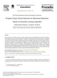
Figure 1: This figure presents the flow of the proposed framework. 1. A small set of labeled data is used to obtain the initial relationship (R) and classification model (C). 2. As new unlabeled batch of data becomes available sequentially over time, we first extract features from the raw data. Then the current C and R models are used to construct a graph from the data to represent the relationships between the data points. Then inference on the graph is used to obtain the node and edge probabilities, which are used to choose the informative samples for manual labeling. The newly labeled instances are then used to update the models C and R. each data point, but also plays an important role in selecting a small subset of informative samples, which when labeled can help the other unlabeled samples to have a better understanding of their labels. Framework Overview. The flow of the proposed method is pictorially presented in Fig.1. The proposed method starts with a small set of labeled data and uses it to build the classification (C) and relationship (R) models. R represents the underlying structure in the data. It may be noted that the classification models may contain multiple classifiers for multiple recognition tasks. After learning the initial models, given a batch of unlabeled samples, the goal is to select a subset of informative samples for manual labeling which can be used to update the current classification and relationship models. As new batch of data becomes available, they are separated into different sets based on the recognition task to which they belong and their features are extracted. Using the current classifiers, a probability mass function over the possible classes is obtained for each unlabeled sample. It is used along with R to construct a graph whose nodes represent the samples. A message passing algorithm is used to infer on the graph to obtain the beliefs of each node and the edges of the graphs. An informative theoretic objective function is derived, which utilizes the beliefs to select the informative nodes for manual labeling. The submodular nature of this optimization function allows us to achieve this in a computationally efficient manner. The newly labeled nodes are used to update the models C and R. It may be noted that the number of samples selected per batch is non-uniform, dependent on the information content of each batch. Main Contributions. The main contributions are the following. • We propose a novel generalized active learning framework which exploits the relationships in data to reduce the manual labeling effort. It can be used for both single as well 3139

as multiple inter-related recognition tasks jointly. • Our framework chooses non-uniform number of samples for manual labeling from each batch of data, which is helpful as the amount of information contained in a batch of data varies and it may not be useful to select the same number of samples from each batch. • Unlike other batch mode subset selection algorithms which exploit relationships in data points, the optimization problem in our framework can be proved to be submodular minimization which makes it easy to obtain optimal solutions in polynomial time.

2. Related Works An overview of the approaches which form the core of most active learning (AL) algorithms may be found at [38]. Most AL algorithms involve the uncertainty of the classifier for choosing the informative samples, best vs. second best [29], entropy [30], classifier margin [44] being commonly used measures for classifier uncertainty. Along with classifier uncertainty, diversification in the chosen samples is introduced by using k-means [29] or sparse representative subset selection [13]. The scalability issue in terms of the number of classes was addressed in [22] by asking binary questions to the human. They selected samples from the unlabeled set based on expected misclassification risk and extracted a probabilistically similar image from the labeled set to ask whether they match. Another important concept used in AL is expected model change [6, 43, 23]. Most of the above mentioned works do not consider the relationships between the data points which may be exploited to reduce the amount of manual labeling. In [5], an AL algorithm was proposed which involves uncertainty, committeebased ensembles and community based clustering of networked data. A network based utility score for each sample was proposed in [27] involving neighborhood information

of the networked data. In [41], maximum uncertainty as well as maximum impact on other unlabeled instances was used, where the link information enhances the feature based similarity measure used to capture the impact of a sample. In [31], a hierarchical model for AL was proposed for scene classification where they also query the objects whenever there is a mismatch between the scene label provided by the classifier and human. An AL algorithm for scene and object classification is presented in [2]. Relationship in the feature space was exploited in [32] for AL. The concept of typicality in information theory is exploited in [3] to choose the optimal subset of samples. Recently, in [7], an algorithm for batch mode AL was proposed which uses entropy and Kullback Leibler divergence to select informative and diverse samples. However, these algorithms do not incorporate the propagation of confidence from one sample to the other. Recently, an AL algorithm is presented in [18] for activity recognition. They proposed an objective function based on intuition and provided a greedy solution to optimize it. Our algorithm on the other hand is not only mathematically validated, but also experimentally supported on different applications (beyond activity recognition), including multiple inter-related tasks. Moreover, our AL algorithm is computationally efficient due to the submodularity property and can be applied in scenarios involving joint learning of multiple recognition models. Also, unlike this method, we do not select a fixed number of samples from each batch; rather the number of samples is non-uniform based on the information content of each batch.

3. Data Representation The proposed method for informative sample selection is based on the assumption that the unlabeled data points have an underlying structure, i.e., have relationships among them. We build a graph whose nodes represent the unlabeled samples in order to exploit the relationships between them. The two important measures which represent the graph are node and edge potentials. Our active learning framework can select samples for single as well as multiple joint classification tasks simultaneously if the instances share relationship, e.g., scene-object, object-object, activity-object classification, etc. In order to generalize, let us consider that we have m tasks in hand which share relationships in data. Let us consider that we have a set of baseline classifiers C = {C1 , . . . , Cm } for these m interrelated tasks. The node and edge potentials in the format we use are discussed below. Node Potential. We represent each data point as a node. Consider that we have total n classes {c1 , . . . , cn } for these m classification problems. Consider an indicator function I(.) which takes as input a class name c and provides as output a unit standard basis vector, i.e., I(c = c1 ) = [1, 0 . . . , 0]T . If F j is the feature of node j, 3140

then its node (unary) potential can be expressed as, φj =

m X n X

Cp (F j , ci )I(c = ci )

(1)

p=1 i=1

where Cp (F j , ci ) represents the probability of node j to belong to class ci . Thus, Cp (F j , ci ) = 0 if the training data of Cp does not contain data of class ci . Edge Potential. The edge (pair-wise) potential represents the relationships between the classes. The relationship model R contains the edge potential matrix ψ whose i,j location is the co-occurence frequency [16] of data point of class ci with data point of class cj . Co-occurrence, and thus edge potential, depends on the application and will be discussed in Section 5. The node and edge potentials play an important role in our framework as we use it to construct a graph to represent the relationships between the data points. It may be noted that our framework can be applied to any dataset containing relationships which can be modeled as edge potentials. Graph Construction. Let us consider that we have a set of labeled data instances L. We learn the baseline classification model C and a relationship model R with these labeled data L. Now, consider that a new unlabeled set U of data becomes available with features {F j }N j=1 , N being the size of the set U. Instead of manually labeling this entire unlabeled set, our goal is to reduce the labeling effort by choosing an informative subset of U for manual labeling, such that it helps to improve the current models C and R. We start by constructing a graph G = (V, E) with the instances in U using the current models C and R. Each node in V = {v1 , . . . , vN } represents each data point. The edges E = {(i, j)|vi and vj are linked} represent the relationships between the data points. The link information between the nodes depends on the application and is discussed in Section 5. The nodes are assigned the corresponding node potentials φi and the edges are assigned the edge potential ψ. A message passing algorithm can be used to obtain the node and edge beliefs. In this paper, we use Loopy Belief Propagation (LBP) [35] to accomplish this task. After inference, we obtain the marginal node probabilities and the pair-wise joint distribution of the edges.

4. Selection of Informative Samples In this section, we discuss how we choose the informative samples based on the graphical model constructed from a batch of data. Using the node and edge probabilities, the goal is to choose a small set V l∗ ⊂ V for manual labeling, which will improve the current models C and R. We wish to select a subset of the nodes such that the joint entropy of all the nodes H(V ) is minimized. Below we derive an expression for the joint entropy of the graph G.

Joint Entropy of Nodes. The entropy of each node and the mutual information between a pair of nodes can be expressed  as H(vi ) = E[− log2 pi ] and I(vi , vj ) = E[log2 pij pi pj ] and pi , pj and pij are the node and edge probabilities respectively. The joint entropy of the nodes of the graph G can be expressed as follows, N X (a) H(V ) = H(v1 ) + H(vi |v1 , . . . , vi−1 )

by optimizing an objective function. The main motivation is that the classifier is either confident or will become confident about the set V nl if we gain information about the subset V l . Here l means Labeled and nl means Not Labeled. Let us define the two subgraphs of G as follows: Gl = l (V , E l ) be the subgraph whose nodes will be labeled and Gnl = (V nl , E nl ) be the subgraph which will not be labeled. For the sake of clarity, the following are defined: E l = {(i, j)|(i, j) ∈ E, vi , vj ∈ V l }, E nl = {(i, j)|(i, j) ∈ E, vi , vj ∈ V nl }. Following the above partition, the joint entropy H(V ) can be partitioned as follows, h X i X H(V ) = H(vi ) − I(vj ; vi ) +

i=2 (b)

=H(v1 ) +

N h X

H(vi ) − I(v1 , . . . , vi−1 ; vi )

i

i=2 (c)

= H(v1 ) +

N h i i X X H(vi ) − I(vj ; vi |v1 , . . . , vj−1 ) i=2

=

N X

H(vi ) −

i=1 (d)

≈

X vi ∈V

vi ∈V l

h X

j=1 N X i X

H(vi ) −

X

H(vi ) −

I(vj ; vi |v1 , . . . , vj−1 )

= H(V l ) + H(V nl ) − I(vj ; vi )

i I(vj ; vi ) −

(i,j)∈E nl

vi ∈V nl

i=2 j=1

(i,j)∈E l

X

(2)

X

I(vj ; vi )

(i,j)∈E vi ∈V l ,vj ∈V nl

X

I(vj ; vi )

(3)

(i,j)∈E vi ∈V l ,vj ∈V nl

(i,j)∈E

(a) Joint entropy chain rule [10] I(v1 , . . . , vj−1 ; vj ) = H(vj ) − (b) Using H(vj |v1 , . . . , vj−1 ), where, I(.; .) represents the mutual information between the set of random variables separated by ’;’. (c) Mutual information chain rule [10] (d) Computing the conditional mutual information I(vj ; vi |v1 , . . . , vj−1 ) becomes computationally intractable as the number of nodes on which it is conditioned increases. Moreover, in this paper, we construct our graph using just unary (node) and pair-wise (edge) potentials and ignoring higher order potentials. Thus, we approximate the conditional mutual information as I(vj ; vi |v1 , . . . , vj−1 ) ≈ I(vj ; vi ). Furthermore, we consider two nodes to be independent if there exist no link between them. It is also known that the mutual information between two random variables is zero, if they are independent. The expression in Eqn 2 is similar to the expression of joint entropy using Bethe Approximation [47]. Moreover, this expression is exact for an acyclic graph but an approximation in case of graphs containing cycles. We use this expression to derive an objective function to be optimized in order to obtain the most informative nodes for manual labeling. Objective Function Derivation. Our goal is to choose a subset of nodes from V , the size of which may vary across each batch of data, such that the joint entropy H(V ) in Eqn. 2 is minimized after inferring on the graph G conditioned on the obtained labels of the chosen nodes. The set V can be partitioned into two sets, V l which will be selected for manual labeling and V nl which will not be manually labeled. We need to find the optimal partition of V into these two sets 3141

Once the nodes in V l are manually labeled and we run inference on the graph conditioned on the acquired labels, the first and last term of the above expression becomes zero (see supplementary material). Most active learning algorithms assume that for each batch of unlabeled data, there is a fixed budget, i.e., number of samples for manual labeling. If the budget for manual labeling is K(≤ N ), then the optimal subset V l∗ which minimizes the joint entropy of the node can be expressed as,h i X V l∗ = arg max H(V l ) − I(vj ; vi ) (4) Vl s.t.|V l |=K

(i,j)∈E vi ∈V l ,vj ∈V nl

However, each batch of data may contain non-uniform amount of information and choosing the same number of budget constrained samples (i.e., K) from each batch may not be a good idea. Instead, the number of samples could be determined based on the information content of each batch. This motivates us to modify the above objective function, such that we choose non-uniform number of informative samples from different batch of data. We rewrite Eqn. 4 as an unconstrained minimization problem as follows: h i X V l∗ = arg min I(vj ; vi ) − H(V l ) + λ|V l | Vl

(i,j)∈E vi ∈V l ,vj ∈V nl

(5) where λ is a positive trade-off parameter between maximizing the objective function in Eqn. 4 and minimizing the number of nodes chosen for manual labeling. The choice of λ is discussed at the end of this section. The optimization problem can be represented in vector and matrix notations. In order to do so, we define the following. Consider a vector x of length N with elements being 1

or 0, where 1 represents the node is selected to be in the set V l and 0 represents the opposite. We need to find the optimal x which solves the optimization problem in Eqn. 5. Let us define a N × 1 vector h of node entropies and a N × N matrix M of pairwise mutual informations as follows, h , [H(v1 ), H(v2 ) . . . H(vN )]T ( I(vi ; vj ), if (i, j) ∈ E M (i, j) , 0, otherwise

1 x = arg min xT Qx + xT f + λxT 1 2 x

v4

v5

v6 X

v8

S

v v7

Algorithm 1 Proposed Framework

(6)

where Q , −M and f , M 1 − h and where 1 = [1 1 . . . 1]T of size N × 1. The objective function in Eqn. 6 can be proved to be submodular which makes the optimization problem simpler compared to Eqn. 4. Details of the optimization is discussed next. Proof of Submodularity. A submodular function is a set function f : P(S) → R where P(S) is the power set of a finite set S, if it satisfies the following, f (X ∪ {v}) − f (X) ≥ f (Y ∪ {v}) − f (Y )

v1

Y

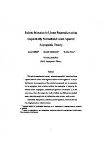
Figure 2: This figure is an example illustration of the sets S, X, Y and the element v involved in proving that the proposed objective function is submodular.

where i, j ∈ {1, . . . , N }. The objective function in Eqn. 5 can be represented as (see supplementary material) ∗

v3

v2

(7)

where X ⊆ Y ⊆ S and v ∈ S − Y . The sets are represented in Fig. 2. Let us consider two vectors x and y representing the two sets X and Y , i.e., if a node exists in a set, the corresponding element of the vector will be 1 else 0. Consider a vector v which represents the node v of Eqn. 7, i.e., v is a vector of all zeros and one at the v th element location. Consider the objective function in Eqn. 6 be f . Then, h1 f (X ∪ {v}) − f (X) = (x + v)T Q(x + v)+ 2 i h1 i T T (x + v) f + λ(x + v) 1 − xT Qx + xT f + λxT 1 2 1 T T T = v Qv + x Qv + v f + λ (8) 2 Also, f (Y ∪ {v}) − f (Y ) = 12 v T Qv + y T Qv + v T f + λ {f (X∪{v})−f (X)}−{f (Y ∪{v})−f (Y )} = (x−y)T Qv (9) Now, as X ⊆ Y , y contains 1 at least in the positions where x contains 1. Thus, the entries of the vector x − y are either 0 or −1. Also, the entries of Q are non-positive as Q = −M and mutual information is always non-negative. Also, v is a vector of 1 at a single element and 0 otherwise. Thus, (x − y)T Qv ≥ 0 and Eqn. 7 is satisfied, which makes the objective function in Eqn. 6 submodular and the optimization problem is submodular minimization. Optimization Procedure. Submodular Function Minimization (SFM) often arises in fields of machine learning, 3142

Input: Sequential Batch of Unlabeled Data {U1 , U2 , . . . }. Output: Classification C and Relationship R models after processing every batch of data. Variable L: Labeled Set, k: batch number 1. L ← U1 : Ask human to label the first batch U1 . 2. Construct the models C and R using L. k←2
while New batch of data Uk available do 3. Construct graph G = (V, E) based on Uk 4. Use the current model C and R to assign the node and edge potentials to the graph 5. Run inference on the graph to obtain the node (pi ) and edge (pij ) probabilities 6. Compute the entropy and mutual information and construct the vector h and matrix M respectively. 7. Find λ using Eqn. 10 8. Obtain x∗ Eqn. 6 using Fujishige-Wolfe Min Norm Point algorithm 9. Use x∗ to select the samples for query to human lets denote it by V l∗ . Then, L ← L ∪ V l∗ 10. Inference conditioned on the acquired labels and L ← L ∪ {Highly confident instances} (weak teacher) 11. Use L to update the models C and R k ←k+1 end while

game theory, information theory, etc. Detailed description may be found here [33]. There exists some algorithms which can be used to solve SFM in polynomial time. We use the Fujishige-Wolfe Min Norm Point algorithm [15] in the Submodular Function Optimization (SFO) [25] toolbox to solve the submodular minimization problem in Eqn. 6. It is one of the most well-known algorithms to solve SFM. Parameter. The parameter λ in Eqn. 6 is a trade-off between the two objectives as discussed previously. If f (x) is the objective function in Eqn. 6, then λ can be expressed as, minx f (x)|λ=0 − 0 λ=α (10) 0 − maxx xT 1 where α is a scalar parameter. In Eqn. 10, a fraction is

obtained using the range of values of the two objective functions, such that the scaling between the two objective functions using λ is appropriate. λ now depends on α, which can be kept close to 1 for all applications due to the scaling done in Eqn. 10 between the two objective functions. Model Update After the chosen samples are labeled by a human, we perform inference on the graph conditioned on the acquired labels to update the beliefs of the nodes and then we apply the concept of weak teacher [51], which does not involve the human. We choose those nodes having confidence of classification > , with the corresponding label, to be in the labeled set L.  should be high enough to avoid wrong labeling. The classification model C is updated by retraining the classifier using L. Model R is comprised of only the co-occurrence matrix ψ and it is incremented using the new labeled instances. An overview of the entire framework is presented in Algorithm 1. Special Case of Archived Data. The proposed method can also be used in cases where the entire dataset is available at the outset (see supplementary material). A small set of samples is randomly selected from the unlabeled dataset and their labels are obtained. These labeled samples are used to construct the initial models C and R. These models are used to choose the informative samples from the rest of the unlabeled pool of samples and then the models are updated after acquiring the labels. This process continues until the joint entropy of the remaining subset < threshold.

5. Experiments In this section, we present experimental analysis of our proposed active learning framework for three distinct applications - joint scene-object classification, activity recognition, and document classification. These applications are chosen as they have data which share relationships among them. For each application, we perform the following experiments. • We compare the proposed method with commonly used and state-of-the-art active learning methods namely Batch Rank [7], BvSB [29], Entropy [39, 19], Density Based Sampling (DENS) [39], Expected Gradient Length (GRL) [40] and Random Sampling. We also compare with CAAL [18] for activity recognition. • We compare the results of our algorithm with other stateof-the-art methods which use the entire dataset for training, details of which is mentioned subsequently. • We perform sensitivity analysis of the proposed method on the parameter α in Eqn. 10. We use Support Vector Machine (SVM) [8] as a baseline classifier for our proposed method as well as for all the active learning methods with which we compare, to have a fair comparison. We use the Undirected Graphical Model (UGM) toolbox [35] to perform inference on the graph. We will use the following short-notations. “ALL” represents the accuracy

obtained by using the entire dataset for training.“ALL Batch” denotes that the classifier is updated using ALL the instances of the current batch.

5.1. Scene-Object Classification Scene and objects tend to co-occur in images. Although, scene and objects classifiers are separate, their joint understanding can be beneficial [50], which can be exploited in our active learning framework to reduce manual labeling. Dataset. We have used the SUN dataset [9, 48] for our experiments on scene-object classification. We use the portion of the dataset which has both scene and object annotations as we aim to exploit their relationship. In order to represent the scene nodes, we extract CNN features (∈ R4096×1 ) from fc-7 layer of VGG-net [52] pre-trained on the places-205 dataset. We use the pipeline of R-CNN [17] to detect the objects and then extract CNN features from fc-7 layer of Alex-net [26], pre-trained on ImageNet [12]. Experimental Set-up. We perform 5 Fold Cross Validatio0 (FCV)n for this dataset. The training data of 4 folds is divided into 6 batches and fed sequentially to our active learning framework. We consider that the first batch is manually labeled and use it to construct the initial models C and R. We assume that the other batch of data are unlabeled and we choose only the informative samples for manual labeling, which is then used to update the models. It may be noted that this application is an example which depicts that our algorithm can be applied for active learning of different recognition tasks jointly. Each image is represented by a single scene node and multiple object nodes as detected by the detector. The graph for this application is considered to be fully connected and the i, j position of the edge potential matrix is a count of the number of times an object of class i appears in a scene of class j. Results. Fig. 3a and 3d presents the comparison of the proposed method with other state-of-the-art active learning methods. The proposed method performs better than the other methods and reaches the “ALL” mark with only 41% and 62% manual labeling for scene and objects respectively. Fig. 3b and 3e presents the results of the proposed method along with methods which consider that the entire dataset is manually labeled and available for training. We compare with SUN-CNN [52] for scene classification and with RCNN [17] and DPM [14] for object classification. As may be observed, the proposed method requires much lesser number of samples to be manually labeled to obtain the same accuracy as“ALL Batch”. Fig. 3c and 3f present the results of the proposed method for different values of the parameter α in Eqn. 10. It may be noted that α = 1.1 have been used for all the results corresponding to the SUN dataset.

3143

75

75 74

65

60 20

Accuracy

72 Proposed Batch Rank BvSB Entropy DENS GRL Random ALL

Accuracy

Accuracy

70 70

Proposed ALL Batch SUN-CNN 65

30 40 50 Percentage of Manual Labeling

20

40 60 80 Percentage of Manual Labeling

(a)

30

20

50

45

45

40

40

35 30 Proposed ALL Batch R-CNN DPM

20

20 30 40 50 Percentage of Manual Labeling

15

60

20

40 60 80 Percentage of Manual Labeling

(d)

30 40 50 Percentage of Manual Labeling

60

(c)

50

25

20

66

100

Accuracy

Accuracy

Accuracy

40

α=0.5 α=0.7 α=1.1 α=1.3

68

(b)

Proposed Batch Rank BvSB Entropy DENS GRL Random ALL

50

70

35 30 25

α=0.5 α=0.7 α=1.1 α=1.3

20 15

100

20

(e)

30 40 50 60 Percentage of Manual Labeling

70

(f)

Figure 3: This figure presents the results on the SUN dataset for joint scene object classification. The top and bottom row presents plots for scene and object respectively. (a), (d) presents the comparison of the proposed method with other active learning methods. (b), (e) presents the comparison with other methods which use the entire dataset for training. (c), (f) presents the sensitivity of the proposed method to the parameter α. 75

75

Proposed Batch Rank BvSB Entropy DENS GRL Random ALL

65

60 10

20 30 40 Percentage of Manual Labeling

Accuracy

70 Accuracy

Accuracy

70

75

65 Proposed ALL Batch CCND LBC

60 20

40 60 80 Percentage of Manual Labeling

(b)

(a)

70

65 α α α α

60 100

10

= 0.5 = 0.7 = 1.1 = 1.3

20 30 40 50 60 Percentage of Manual Labeling

(c)

Figure 4: This figure presents the results on the CORA dataset for document classification. (a) presents the comparison of the proposed method with other active learning methods. (b) presents the comparison with other methods which use the entire dataset for training. (c) presents the sensitivity of the proposed method to the parameter α.

5.2. Document Classification Documents are generally inter-linked by citations and hyperlinks, which may be exploited using our active learning approach to reduce manual labeling effort. Dataset. We use the CORA dataset [37] for our experiments on document classification. It is a dataset containing 2708 scientific publications divided into seven classes. There are a total of 5429 links (citations) between the publications. The publications are represented using a dictionary of 1433 unique words and the feature vectors F i ∈ {0, 1}1433 indicate the absence or presence of these words. 3144

Experimental Set-up. We perform 10 FCV for this dataset following [37] and follow a similar set-up as discussed previously for scene-object. We construct the graph such that each node is connected to its five nearest neighbor in the feature space. The i, j position of the edge potential matrix is a count of the number of times a publication belonging to class i is related to class j via a citation link. Results. The results of the proposed AL method along with other state-of-the art AL methods is presented in Fig. 4a. It may be observed that the proposed method performs much better than the other algorithms and requires only 42% manual labeling to reach “ALL”.

Proposed CAAL Batch Rank BvSB Entropy DENS GRL Random ALL

65 60 55 50 10

15 20 25 30 35 Percentage of Manual Labeling

40

75

75

70

70 Accuracy

Accuracy

70

Accuracy

75

65 60 Proposed ALL Batch CAAR SPN

55 50 20

40 60 80 Percentage of Manual Labeling

(b)

(a)

100

65 60 α α α α

55 50

10

15 20 25 30 35 Percentage of Manual Labeling

= 0.5 = 0.9 = 1.2 = 1.4 40

(c)

Figure 5: This figure presents the results on the VIRAT dataset for activity classification. (a) presents the comparison of the proposed method with other active learning methods. (b) presents the comparison with other methods which use the entire dataset for training. (c) presents the sensitivity of the proposed method to the parameter α. We also compare our proposed method with other methods which consider that the entire dataset is manually labeled and use it for training. Fig. 4b presents the comparison with two such methods namely CCND [37] and LBC [36] 1 . The proposed method performs much better than “ALL Batch”, which signifies that the proposed method extracts maximum possible information from the unlabeled set, but using much lesser manual labeling. We also present analysis of the parameter α in Eqn. 10 and the plots are presented in Fig. 4c. The results in Fig. 4a and 4b is with α = 1.1. Lower the value of α, lesser will be the penalty for the number of samples chosen per batch (Eqn. 6), thus more samples will be chosen. This is also evident from Fig. 4c. Although, the performance with α = 0.5 is similar to α = 1.1 at the end, the later chooses much lesser number of samples for manual labeling.

5.3. Activity Classification Activities are generally spatially-temporally related which can be exploited to reduce the number of instances chosen for manual labeling. Dataset. We use the VIRAT dataset [34] on human activity for our experiments on activity classification. The dataset consists of 11 videos segmented into 329 activity sequences. We extracted features using the pre-trained model of 3D convolutional networks [42]. We extract the features from 16 frames with a temporal stride of 8 and then apply max pooling to obtain a single vector ∈ R4096 for each activity. Experimental Set-up. We have used the first 176 sequence (761 activities) for training and 153 sequence (661 activities) for testing. We have divided the training set into 20 batches and fed them sequentially to our active learning algorithm. We consider that there exists a link between two activities if they have occurred within a certain spatiotemporal distance. We consider the edge potential to be the spatio-temporal co-occurrence between the two activities.

Results. The results of the proposed active learning algorithm with other state-of-the-art active learning methods is presented in Fig. 5a. It may be observed that the proposed method not only reaches the accuracy of “ALL” in only 18% manual labeling, but also performs better than “ALL”. The fact that an algorithm can perform better than “ALL”, i.e. using the entire dataset for training is discussed in [28]. Although Batch Rank reaches “ALL”, it requires much more manual labeling than required by the proposed method. ”CAAL” remains close to the proposed algorithm initially, but the latter peaks up thereafter. We compare the proposed method in in Fig. 5b with other learning algorithms which consider the entire dataset to be manually labeled and use it for training namely - Context Aware Activity Recognition (CAAR) [53] and Sum Product Network (SPN) [1]. It may be observed that the proposed method peaks much faster than “ALL Batch” which indicates that the former requires lesser manual labeling in each batch to obtain the same accuracy as when the entire batch is manually labeled and used for training. The plots for sensitivity analysis of the parameter α for the VIRAT dataset is presented in Fig. 5c.

1 Please note that the horizontal lines should be points at 100% manual labeling, but for the sake of clarity, we have presented them as it is.

3145

6. Conclusions and Future Work In this paper, we proposed a novel generalized active learning framework for inter-related data. Our framework can be applied for active learning of both single as well as multiple recognition tasks simultaneously by exploiting the inter-relationships in data. Our proposed method selects nonuniform number of samples from each batch depending on the information content. The proposed informative subset selection methodology is not only fast due to its submodular property, but also performs well on a wide range of applications. Future work will consider the scenario where the labels provided by human is not always correct. Acknowledgments. This work was partially supported by ONR contract N00014-15-C-5113 through a sub-contract from Mayachitra Inc.

References [1] M. R. Amer and S. Todorovic. Sum-product networks for modeling activities with stochastic structure. In Computer Vision and Pattern Recognition(CVPR), pages 1314–1321. IEEE, 2012. [2] J. H. Bappy, S. Paul, and A. K. Roy-Chowdhury. Online adaptation for joint scene and object classification. In European Conference on Computer Vision(ECCV), pages 227–243. Springer, 2016. [3] J. H. Bappy, S. Paul, E. Tuncel, and A. K. Roy-Chowdhury. The impact of typicality for informative representative selection. In Computer Vision and Pattern Recognition(CVPR). IEEE, 2017. [4] M. Bilgic and L. Getoor. Link-based active learning. In NIPS Workshop on Analyzing Networks and Learning with Graphs, 2009. [5] M. Bilgic, L. Mihalkova, and L. Getoor. Active learning for networked data. In International Conference on Machine Learning(ICML), pages 79–86, 2010. [6] W. Cai, Y. Zhang, and J. Zhou. Maximizing expected model change for active learning in regression. In International Conference on Data Mining(ICDM), pages 51–60. IEEE, 2013. [7] S. Chakraborty, V. Balasubramanian, Q. Sun, S. Panchanathan, and J. Ye. Active batch selection via convex relaxations with guaranteed solution bounds. Transactions on Pattern Analysis and Machine Intelligence(TPAMI), 37(10):1945– 1958, 2015. [8] C.-C. Chang and C.-J. Lin. Libsvm: a library for support vector machines. Transactions on Intelligent Systems and Technology (TIST), 2(3):27, 2011. [9] M. J. Choi, J. J. Lim, A. Torralba, and A. S. Willsky. Exploiting hierarchical context on a large database of object categories. In Computer vision and pattern recognition (CVPR), pages 129–136. IEEE, 2010. [10] T. M. Cover and J. A. Thomas. Elements of information theory. John Wiley & Sons, 2012. [11] N. V. Cuong, W. S. Lee, N. Ye, K. M. A. Chai, and H. L. Chieu. Active learning for probabilistic hypotheses using the maximum gibbs error criterion. In Advances in Neural Information Processing Systems(NIPS), pages 1457–1465, 2013. [12] J. Deng, W. Dong, R. Socher, L.-J. Li, K. Li, and L. FeiFei. Imagenet: A large-scale hierarchical image database. In Computer Vision and Pattern Recognition (CVPR), pages 248–255. IEEE, 2009. [13] E. Elhamifar, G. Sapiro, A. Yang, and S. Shankar Sasrty. A convex optimization framework for active learning. In International Conference on Computer Vision(ICCV), pages 209–216. IEEE, 2013. [14] P. F. Felzenszwalb, R. B. Girshick, D. McAllester, and D. Ramanan. Object detection with discriminatively trained partbased models. Transactions on Pattern Analysis and Machine Intelligence(TPAMI), 32(9):1627–1645, 2010. [15] S. Fujishige, T. Hayashi, and S. Isotani. The minimum-normpoint algorithm applied to submodular function minimization and linear programming. Citeseer, 2006.

3146

[16] C. Galleguillos, A. Rabinovich, and S. Belongie. Object categorization using co-occurrence, location and appearance. In Computer Vision and Pattern Recognition(CVPR), pages 1–8. IEEE, 2008. [17] R. Girshick, J. Donahue, T. Darrell, and J. Malik. Rich feature hierarchies for accurate object detection and semantic segmentation. In Computer Vision and Pattern Recognition(CVPR), pages 580–587. IEEE, 2014. [18] M. Hasan and A. K. Roy-Chowdhury. Context aware active learning of activity recognition models. In International Conference on Computer Vision(ICCV), pages 4543–4551. IEEE, 2015. [19] A. Holub, P. Perona, and M. C. Burl. Entropy-based active learning for object recognition. In Computer Vision and Pattern Recognition Workshops(CVPRW), pages 1–8. IEEE, 2008. [20] X. Hu, J. Tang, H. Gao, and H. Liu. Actnet: Active learning for networked texts in microblogging. In SIAM International Conference on Data Mining(SDM), pages 306–314. SIAM, 2013. [21] A. Jain, A. R. Zamir, S. Savarese, and A. Saxena. Structuralrnn: Deep learning on spatio-temporal graphs. arXiv preprint arXiv:1511.05298, 2015. [22] A. J. Joshi, F. Porikli, and N. P. Papanikolopoulos. Scalable active learning for multiclass image classification. Transactions on Pattern Analysis and Machine Intelligence(TPAMI), 34(11):2259–2273, 2012. [23] C. K¨ading, A. Freytag, E. Rodner, A. Perino, and J. Denzler. Large-scale active learning with approximations of expected model output changes. In German Conference on Pattern Recognition(GCPR), pages 179–191. Springer, 2016. [24] H. S. Koppula, R. Gupta, and A. Saxena. Learning human activities and object affordances from rgb-d videos. International Journal of Robotics Research (IJRR), 32(8):951–970, 2013. [25] A. Krause. Sfo: A toolbox for submodular function optimization. Journal of Machine Learning Research, 11(Mar):1141– 1144, 2010. [26] A. Krizhevsky, I. Sutskever, and G. E. Hinton. Imagenet classification with deep convolutional neural networks. In Advances in Neural Information Processing Systems(NIPS), pages 1097–1105, 2012. [27] A. Kuwadekar and J. Neville. Relational active learning for joint collective classification models. In International Conference on Machine Learning(ICML), pages 385–392, 2011. [28] A. Lapedriza, H. Pirsiavash, Z. Bylinskii, and A. Torralba. Are all training examples equally valuable? arXiv preprint arXiv:1311.6510, 2013. [29] X. Li, R. Guo, and J. Cheng. Incorporating incremental and active learning for scene classification. In Machine Learning and Applications (ICMLA), volume 1, pages 256–261. IEEE, 2012. [30] X. Li and Y. Guo. Adaptive active learning for image classification. In Computer Vision and Pattern Recognition(CVPR), pages 859–866, 2013.

[31] X. Li and Y. Guo. Multi-level adaptive active learning for scene classification. In European Conference on Computer Vision(ECCV), pages 234–249. Springer, 2014. [32] O. Mac Aodha, N. D. Campbell, J. Kautz, and G. J. Brostow. Hierarchical subquery evaluation for active learning on a graph. In Computer Vision and Pattern Recognition(CVPR), pages 564–571. IEEE, 2014. [33] S. T. McCormick. Submodular function minimization. Handbooks in Operations Research and Management Science, 12:321–391, 2005. [34] S. Oh, A. Hoogs, A. Perera, N. Cuntoor, C.-C. Chen, J. T. Lee, S. Mukherjee, J. Aggarwal, H. Lee, L. Davis, et al. A largescale benchmark dataset for event recognition in surveillance video. In Computer Vision and Pattern Recognition(CVPR), pages 3153–3160. IEEE, 2011. [35] M. Schmidt. Ugm: A matlab toolbox for probabilistic undirected graphical models, 2007. [36] P. Sen and L. Getoor. Link-based classification. 2007. [37] P. Sen, G. Namata, M. Bilgic, L. Getoor, B. Galligher, and T. Eliassi-Rad. Collective classification in network data. AI magazine, 29(3):93, 2008. [38] B. Settles. Active learning literature survey. University of Wisconsin, Madison, 52(55-66):11, 2010. [39] B. Settles. Active learning. Synthesis Lectures on Artificial Intelligence and Machine Learning, 6(1):1–114, 2012. [40] B. Settles and M. Craven. An analysis of active learning strategies for sequence labeling tasks. In Empirical Methods in Natural Language Processing (EMNLP), pages 1070–1079. Association for Computational Linguistics, 2008. [41] L. Shi, Y. Zhao, and J. Tang. Batch mode active learning for networked data. ACM Transactions on Intelligent Systems and Technology (TIST), 3(2):33, 2012. [42] D. Tran, L. Bourdev, R. Fergus, L. Torresani, and M. Paluri. Learning spatiotemporal features with 3d convolutional networks. In International Conference on Computer Vision (ICCV), pages 4489–4497. IEEE, 2015. [43] A. Vezhnevets, J. M. Buhmann, and V. Ferrari. Active learning for semantic segmentation with expected change. In Computer Vision and Pattern Recognition(CVPR), pages 3162– 3169. IEEE, 2012. [44] S. Vijayanarasimhan and K. Grauman. Large-scale live active learning: Training object detectors with crawled data and crowds. International Journal of Computer Vision(IJCV), 108(1-2):97–114, 2014. [45] B. Wang, D. Lin, H. Xiong, and Y. Zheng. Joint inference of objects and scenes with efficient learning of text-object-scene relations. Transactions on Multimedia(TMM), 18(3):507–520, 2016. [46] Z. Wang, Q. Shi, C. Shen, and A. Van Den Hengel. Bilinear programming for human activity recognition with unknown mrf graphs. In Computer Vision and Pattern Recognition(CVPR), pages 1690–1697, 2013. [47] A. Weller, K. Tang, D. Sontag, and T. Jebara. Understanding the bethe approximation: when and how does it go wrong? [48] J. Xiao, J. Hays, K. A. Ehinger, A. Oliva, and A. Torralba. Sun database: Large-scale scene recognition from abbey to zoo. In Computer vision and pattern recognition (CVPR), pages 3485–3492. IEEE, 2010.

3147

[49] B. Yao and L. Fei-Fei. Modeling mutual context of object and human pose in human-object interaction activities. In Computer Vision and Pattern Recognition(CVPR), pages 17– 24. IEEE, 2010. [50] J. Yao, S. Fidler, and R. Urtasun. Describing the scene as a whole: Joint object detection, scene classification and semantic segmentation. In Computer Vision and Pattern Recognition(CVPR), pages 702–709. IEEE, 2012. [51] C. Zhang and K. Chaudhuri. Active learning from weak and strong labelers. In Advances in Neural Information Processing Systems, pages 703–711, 2015. [52] B. Zhou, A. Lapedriza, J. Xiao, A. Torralba, and A. Oliva. Learning deep features for scene recognition using places database. In Advances in Neural Information Processing Systems(NIPS), pages 487–495, 2014. [53] Y. Zhu, N. M. Nayak, and A. K. Roy-Chowdhury. Contextaware modeling and recognition of activities in video. In Computer Vision and Pattern Recognition(CVPR), pages 2491– 2498. IEEE, 2013.