Jan 22, 2014 - X =PSX. (18). The following theorem demonstrates that the noisy d-tilted information exhibits properties similar to ...... IL, Oct. 2000, pp. 368â377 ...
1
Nonasymptotic noisy lossy source coding Victoria Kostina, Sergio Verd´u
arXiv:1401.5125v1 [cs.IT] 20 Jan 2014
Dept. of Electrical Engineering, Princeton University, NJ 08544, USA
Abstract This paper shows new general nonasymptotic achievability and converse bounds and performs their dispersion analysis for the lossy compression problem in which the compressor observes the source through a noisy channel. While this problem is asymptotically equivalent to a noiseless lossy source coding problem with a modified distortion function, nonasymptotically there is a noticeable gap in how fast their minimum achievable coding rates approach the rate-distortion function, providing yet another example in which at finite blocklengths one must put aside traditional asymptotic thinking.
Index Terms Achievability, converse, finite blocklength regime, lossy data compression, noisy source coding, strong converse, dispersion, memoryless sources, Shannon theory.
I. I NTRODUCTION Consider a lossy compression setup in which the encoder has access only to a noise-corrupted version X of a source S, and we are interested in minimizing (in some stochastic sense) the distortion d(S, Z) between the true source S and its rate-constrained representation Z (see Fig. 1). This problem arises if the object to be compressed is the result of an uncoded transmission over a noisy channel, or if it is observed data subject to errors inherent to the measurement system. Examples include speech in a noisy environment and photographs corrupted by noise introduced by the image sensor. Since we are concerned with reproducing the original noiseless This work was supported in part by the National Science Foundation (NSF) under Grant CCF-1016625 and by the Center for Science of Information (CSoI), an NSF Science and Technology Center, under Grant CCF-0939370. This work was presented in part at the 2013 IEEE Information Theory Workshop [1].
January 22, 2014
DRAFT
2
source rather than preserving the noise, the distortion measure is defined with respect to the source. The noisy source coding setting was introduced by Dobrushin and Tsybakov [2], who showed that when the goal is to minimize the average distortion, the noisy source coding problem is asymptotically equivalent to a surrogate noiseless source coding problem. Specifically, for a stationary memoryless source with single-letter distribution PS observed through a stationary memoryless channel with single-input transition probability kernel PX|S , the noisy rate-distortion function under a separable distortion measure is given by R(d) =
=
min
I(X; Z)
(1)
min
I(X; Z)
(2)
PZ|X : E[d(S,Z)]≤d S−X−Z
PZ|X : ¯ E[d(X,Z) ]≤d
where the surrogate per-letter distortion measure is ¯d(a, b) = E [d(S, b)|X = a] .
(3)
Therefore, in the limit of infinite blocklengths, the problem is equivalent to a conventional (noiseless) lossy source coding problem where the distortion measure is the conditional average of the original distortion measure given the noisy observation of the source. Berger [3, p.79] used the surrogate distortion measure (3) to streamline the proof of (2). Witsenhausen [4] explored the capability of distortion measures defined through conditional expectations such as in (3) to treat various so-called indirect rate distortion problems. Sakrison [5] showed that if both the source and its noise-corrupted version take values in a separable Hilbert space and the fidelity criterion is mean-squared error, then asymptotically, an optimal code can be constructed by first obtaining a minimum mean-square estimate of the source sequence based on its noisy observation, and then compressing the estimated sequence as if it were noise-free. Wolf and Ziv [6] showed that Sakrison’s result holds even nonasymptotically, namely, that the minimum average distortion achievable in one-shot noisy compression of the object S can be written as � � � � D ⋆ (M) = E |S − E [S|X] |2 + inf E |c(f(X)) − E [S|X] |2 f,c
(4)
where the infimum is over all encoders f : X 7→ {1, . . . , M} and all decoders c : {1, . . . , M} 7→ c and X and M c are the alphabets of the channel output and the decoder output, respectively. It M,
January 22, 2014
DRAFT
3
is important to note that the choice of the mean-squared error distortion is crucial for the validity of the additive decomposition in (4). For vector quantization of a Gaussian signal corrupted by an additive independent Gaussian noise under weighted squared error distortion measure, Ayanoglu [7] found explicit expressions for the optimum quantization rule. Wolf and Ziv’s result was extended to waveform vector quantization under weighted quadratic distortion measures and to autoregressive vector quantization under the Itakura-Saito distortion measure by Ephraim and Gray [8], and by Fisher, Gibson and Koo [9], who studied a model in which both encoder and decoder have access to the history of their past input and output blocks, allowing exploitation of inter-block dependence. Thus, the cascade of the optimal estimator followed by the optimal compressor achieves the minimum average distortion in those settings as well. Under the logarithmic loss distortion measure [10], the noisy source coding problem reduces to the information bottleneck problem [11]. Indeed, in the information bottleneck method, the goal is to minimize I(X; Z) subject to the constraint that I(S; Y ) exceeds a certain threshold. On the other hand, the noisy rate-distortion function under logarithmic loss is given by (2) in which � � E ¯d(X, Z) is replaced by H(S|Y). The two optimization problems are equivalent. The solution
to the information bottleneck problem thus acquires an operational meaning of the asymptotically minimum achievable noisy source coding rate under logarithmic loss. In this paper, we give new nonasymptotic achievability and converse bounds for the noisy source coding problem, which generalize the noiseless source coding bounds in [12]. We ob-
serve that at finite blocklenghs, the noisy coding problem is, in general, not equivalent to the noiseless coding problem with the surrogate distortion measure. Essentially, the reason is that taking the expectation in (3) dismisses the randomness introduced by the noisy channel, which nonasymptotically cannot be neglected. The additional randomness introduced by the channel slows down the rate of approach to the asymptotic fundamental limit in the noisy source coding problem compared to the asymptotically equivalent noiseless problem. Specifically, for noiseless source coding of stationary memoryless sources with separable distortion measure, we showed previously [12] (see also [13] for an alternative proof in the finite alphabet case) that the minimum number M of representation points compatible with a given probability ǫ of exceeding distortion threshold d can be written as �√ � p −1 k log M (k, d, ǫ) = kR(d) + kV(d)Q (ǫ) + o ⋆
January 22, 2014
(5)
DRAFT
4
100)
{1, . . . , M } X
S Fig. 1.
Y
Noisy source coding.
where V(d) is the rate-dispersion function, explicitly identified in [12], and Q−1 (·) denotes the inverse of the complementary standard Gaussian cdf. In this paper, we show that for noisy source coding of a discrete stationary memoryless source over a discrete stationary memoryless channel under a separable distortion measure, V(d) in (5) is replaced by the noisy rate-dispersion function ˜ V(d), which can be expressed as ˜ V(d) = V(d) + λ⋆2 Var (E [d(S, Z⋆)|S, X] − E [d(S, Z⋆ )|X])
(6)
where λ⋆ = −R′ (d), V(d) is the rate-dispersion function of the surrogate rate-distortion setup,
and Z⋆ denotes the reproduction random variable that achieves the rate-distortion function (2). ˜ The difference between V(d) and V(d) is due to stochastic variability of the channel from S
˜ to X, which nonasymptotically cannot be neglected. Note, also, that V(d) cannot be expressed solely as a function of the source distribution and the surrogate distortion function. The rest of the paper is organized as follows. After introducing the basic definitions in Section
II, we proceed to show new general nonasymptotic converse and achievability bounds in Sections III and IV, respectively, along with their asymptotic analysis in Section V. Finally, the example of a binary source observed through an erasure channel is discussed in Section VI. II. D EFINITIONS Consider the one-shot setup in Fig. 1 where we are given the distribution PS on the alphabet M and the transition probability kernel PX|S : M → X . We are also given the distortion measure c 7→ [0, +∞], where M c is the representation alphabet. An (M, d, ǫ) code is a pair of d: M × M
c such that P [d(S, Z) > d] ≤ ǫ. mappings PU |X : X 7→ {1, . . . , M} and PZ|U : {1, . . . , M} 7→ M Define
RS,X (d) ,
January 22, 2014
inf
PZ|X : d(X,Z)]≤d E[¯
I(X; Z)
(7)
DRAFT
5
c 7→ [0, +∞] is given by where d¯ : X × M
¯ z) , E [d(S, z)|X = x] d(x,
(8)
and, as in [12], assume that the infimum in (7) is achieved by some PZ ⋆ |X such that the constraint is satisfied with equality. Noting that this assumption guarantees differentiability of RS,X (d), denote λ⋆ = −R′S,X (d)
(9)
Furthermore, define, for an arbitrary PZ|X d¯Z (s|x) , E [d(S, Z)|X = x, S = s]
(10)
= E [d(s, Z)|X = x]
(11)
where the expectation is with respect PZ|XS = PZ|X , and (11) follows from S − X − Z. Definition 1 (noisy d-tilted information). For d > dmin, the noisy d-tilted information in s ∈ M given observation x ∈ X is defined as ˜S,X (s, x, d) , D(PZ ⋆ |X=x kPZ ⋆ ) + λ⋆ ¯dZ ⋆ (s|x) − λ⋆ d
(12)
where PZ ⋆ |X achieves the infimum in (7). As we will see, the intuitive meaning of the noisy d-tilted information is the number of bits required to represent s within distortion d given observation x. For the surrogate noiseless source coding problem, we know that almost surely ( [14, Lemma 1.4], [15, Theorem 2.1]) ¯ Z ⋆ ) − λ⋆ d X (x, d) = ıX;Z ⋆ (x; Z ⋆ ) + λ⋆ d(x, � � ¯ Z ⋆ )|X = x − λ⋆ d = D(PZ ⋆ |X=x kPZ ⋆ ) + λ⋆ E d(x,
(13) (14)
¯ where X (x, d) is the d-tilted information in x ∈ X whose intuitive meaning is the number of bits required to represent x within distortion d and which is formally defined in [12, Definition 6]. From (12) and (14), we get � � ˜S,X (s, x, d) = X (x, d) + λ⋆ d¯Z ⋆ (s|x) − λ⋆ E ¯dZ ⋆ (S|x)|X = x January 22, 2014
(15)
DRAFT
6
and RS,X (d) = E [˜ S,X (S, X, d)] = E [X (X, d)]
(16) (17)
If alphabets M and X are finite, for (c, a) ∈ M × X , denote the partial derivatives ˙ S,X (s, x, d) , R
∂ R ¯ ¯ (d) |PS¯X¯ =PSX ∂PS¯X¯ (c, a) S,X
(18)
The following theorem demonstrates that the noisy d-tilted information exhibits properties similar to those of the d-tilted information listed in [15, Theorem 2.2] (reproduced in Theorem 11 in Appendix A). Theorem 1. Assume that M and X are finite sets. Suppose that for all PS¯X¯ in some Euclidean ¯ Z¯ ⋆ ). Then neighborhood of PSX , supp(PZ¯ ⋆ ) = supp(PZ ⋆ ), where RS, ¯X ¯ (d) = I(X; � � ∂ E ˜S, ¯X ¯ (S, X, d) |PS¯X ¯ =PSX = − log e, ∂PS¯X¯ (s, x)
˙ S,X (s, x, d) = ˜S,X (s, x, d) − log e, R � ˙ Var RS,X (S, X, d) = Var (˜ S,X (S, X, d)) . �
(19) (20) (21)
Proof: Appendix B. c and λ > 0 define the transition probability kernel For a given distribution PZ¯ on M � ¯ z) dPZ¯ (z) exp −λd(x, � �� dPZ¯ ⋆ |X=x (z) = ¯ Z) ¯ E exp −λd(x,
(22)
and define the function
where
J˜Z¯ (s, x, λ) , D(PZ¯ ⋆ |X=x kPZ¯ ) + λd¯Z¯ ⋆ (s|x) � � = JZ¯ (x, λ) + λd¯Z¯ ⋆ (s|x) − λE ¯dZ¯ ⋆ (S|x)|X = x JZ¯ (x, λ) , log
1 � �� ¯ E exp −λd(x, Z)
(23) (24)
(25)
where the expectation is with respect to the unconditional distribution of PZ¯ . Similar to [15, (2.26)], we refer to the function J˜Z¯ (s, x, λ) − λd January 22, 2014
(26) DRAFT
7
as the generalized noisy d-tilted information. As in the noiseless case, the generalized d-tilted information turns out to be relevant to the following optimization problem. RS,X;Z¯ (d) ,
inf
PZ|X : ¯ E[d(X,Z) ]≤d
III. C ONVERSE
D(PZ|X kPZ¯ |PX )
(27)
BOUNDS
Our main converse result for the nonasymptotic noisy lossy compression setting is the following lower bound on the excess distortion probability as a function of the code size. Theorem 2 (Converse). Any (M, d, ǫ) code must satisfy � � � � (X; Z) + sup λ(d(S, Z) − d) ≥ log M + γ − exp(−γ) ǫ ≥ inf sup P ıX| ¯ ZkX ¯ PZ|X γ≥0,P ¯ ¯ X|Z
(28)
λ≥0
where (x; z) , log ıX| ¯ ZkX ¯
dPX| ¯ Z=z ¯ (x) dPX
(29)
Proof: Let the encoder and decoder be the random transformations PU |X and PZ|U , where U takes values in {1, . . . , M}. Denote
n o c : d(s, z) ≤ d Bd (s) , z ∈ M
January 22, 2014
(30)
DRAFT
8
We have, for any γ ≥ 0 � � (X; Z) + sup λ(d(S, Z) − d) ≥ log M + γ P ıX| ¯ ZkX ¯ λ≥0
� � (X; Z) + sup λ(d(S, Z) − d) ≥ log M + γ, d(S, Z) > d = P ıX| ¯ ZkX ¯ λ≥0
� � (X; Z) + sup λ(d(S, Z) − d) ≥ log M + γ, d(S, Z) ≤ d + P ıX| ¯ ZkX ¯
(31)
λ≥0
� � (X; Z) ≥ log M + γ, d(S, Z) ≤ d = P [d(S, Z) > d] + P ıX| ¯ ZkX ¯ � � (X; Z) ≥ log M + γ ≤ ǫ + P ıX| ¯ ZkX ¯
�� exp(−γ) � (X; Z) E exp ıX| ¯ ZkX ¯ M M X � exp(−γ) X X ≤ ǫ+ (x; z) PX (x) exp ıX| PZ|U (z|u) ¯ ZkX ¯ M u=1 x∈X ≤ ǫ+
(32) (33) (34) (35)
c z∈M
= ǫ+
M X exp(−γ) X X PZ|U (z|u) PX| ¯ Z ¯ (x|z) M u=1 x∈X
(36)
c z∈M
= ǫ + exp (−γ)
(37)
where •
(32) is by direct solution for the supremum;
•
(34) is by Markov’s inequality;
•
(35) follows by upper-bounding PU |X (u|x) ≤ 1
(38)
for every (x, u) ∈ M × {1, . . . , M}. Finally, (28) follows by choosing γ and PX| ¯ Z ¯ that give the tightest bound and PZ|X that gives the weakest bound in order to obtain a code-independent converse. The following bound reduces the intractable (in high dimensional spaces) infimization over all conditional probability distributions PZ|X in Theorem 2 to infimization over the symbols of the output alphabet.
January 22, 2014
DRAFT
9
Corollary 1. Any (M, d, ǫ) code must satisfy �� � � � � (X; z) + sup λ(d(S, z) − d) ≥ log M + γ|X − exp(−γ) ǫ ≥ sup E inf P ıX| ¯ ZkX ¯ γ≥0,PX| ¯ ¯ Z
c z∈M
λ≥0
(39)
Proof: We weaken (28) using � � (X; Z) + sup λ(d(S, Z) − d) ≥ log M + γ inf P ıX| ¯ ¯ ZkX PZ|X
λ≥0
�� � (X; Z) + sup λ(d(S, Z) − d) ≥ log M + γ|X = E inf P ıX| ¯ ZkX ¯ �
PZ|X
(40)
λ≥0
�� � (X; z) + sup λ(d(S, z) − d) ≥ log M + γ|X = E inf P ıX| ¯ ZkX ¯ �
c z∈M
(41)
λ≥0
where we used S − X − Z. In our asymptotic analysis, we will apply Corollary 1 with suboptimal choices of λ and PX| ¯ Z ¯. ¯ c and PX|S is the identity mapping so that d(S, z) = d(X, z) almost Remark 1. If supp(PZ ⋆ ) = M surely, for every z, then Corollary 1 reduces to the noiseless converse in [12, Theorem 7] by
⋆ using (13) after weakening (39) with PX| ¯ Z ¯ = PX|Z ⋆ and λ = λ .
IV. ACHIEVABILITY
BOUNDS
Theorem 3 (Achievability). There exists an (M, d, ǫ) code with Z 1 � � �� ¯ > t|X dt ǫ ≤ inf E PM π(X, Z) PZ¯
(42)
0
where PX Z¯ = PX PZ¯ , and
π(x, z) = P [d(S, z) > d|X = x]
(43)
Proof: The proof appeals to a random coding argument. Given M codewords (c1 , . . . , cM ), the encoder f and decoder c achieving minimum excess distortion probability attainable with the given codebook operate as follows. Having observed x ∈ X , the optimum encoder chooses i⋆ ∈ arg min π(x, ci ) i
(44)
with ties broken arbitrarily, so f(x) = i⋆ and the decoder simply outputs ci⋆ , so c(f(x)) = ci⋆ . January 22, 2014
DRAFT
10
The excess distortion probability achieved by the scheme is given by P [d(S, c(f(X))) > d] = E [π(X, c(f(X)))] Z 1 = P [π(X, c(f(X))) > t] dt 0 Z 1 = E [P [π(X, c(f(X))) > t|X]] dt
(45) (46) (47)
0
Now, we notice that 1 {π(x, c(f(x))) > t} = 1 =
�
M Y i=1
� min π(x, ci ) > t
i∈1,...,M
1 {π(x, ci ) > t}
(48) (49)
and we average (47) with respect to the codewords Z1 , . . . , ZM drawn i.i.d. from PZ¯ , independently of any other random variable, so that PXZ1 ...ZM = PX × PZ¯ × . . . × PZ¯ , to obtain # Z 1 "Y Z 1 M � � �� ¯ > t|X dt E P [π(X, ZM ) > t|X] dt = E PM π(X, Z) 0
(50)
0
i=1
Since there must exist a codebook achieving excess distortion probability below or equal to the average over codebooks, (42) follows. Remark 2. Notice that we have actually shown that the right-hand side of (42) gives the exact minimum excess distortion probability of random coding, averaged over codebooks drawn i.i.d. from PZ . Remark 3. In the noiseless case, S = X, so almost surely π(X, z) = 1 {d(S, z) > d}
(51)
and the bound in Theorem 3 reduces to the noiseless random coding bound in [12, Theorem 10]. The bound in (42) can be weakened to obtain the following result, which generalizes Shannon’s bound for noiseless lossy compression (see e.g. [12, Theorem 1]). Corollary 2. There exists an (M, d, ǫ) code with � � − exp(γ) ǫ ≤ inf P [d(S, Z) > d] + P [ıX;Z (X; Z) > log M − γ] + e γ≥0, PZ|X
January 22, 2014
(52)
DRAFT
11
where PSXZ = PS PX|S PZ|X . Proof: Fix γ ≥ 0 and transition probability kernel PZ|X . Let PX → PZ|X → PZ (i.e. PZ is the marginal of PX PZ|X ), and let PX Z¯ = PX PZ . We use the nonasymptotic covering lemma [16, Lemma 5] to establish � � �� ¯ > t|X ≤ P [π(X, Z) > t] + P [ıX;Z (X; Z) > log M − γ] + e− exp(γ) E PM π(X, Z)
Applying (53) to (50) and noticing that Z 1 P [π(X, Z) > t] dt = E [π(X, Z)]
(53)
(54)
0
= P [d(S, Z) > d]
(55)
we obtain (52). The following weakening of Theorem 3 is tighter than that in Corollary 2. It uses the generalized d-tilted information and is amenable to an accurate second-order analysis. See [15, Theorem 2.19] for a noiseless lossy compression counterpart. Theorem 4 (Achievability, generalized d-tilted information). Suppose that PZ|X is such that almost surely d(S, Z) = d¯Z (S|X)
(56)
Then there exists an (M, d, ǫ) code with n � n h � E inf P D(PZ|X=x kPZ¯ ) + λd¯Z (S|x) − λ(d − δ) > log γ − log β|X ǫ ≤ inf γ,β,δ,PZ¯
λ>0
� � + P d¯Z (S|X) > d|X o � � + oi M + 1 − βP d − δ ≤ d¯Z (S|X) ≤ d|X | + e− γ
(57)
Note that assumption (56) is satisfied, for example, by any constant composition code PZ k |X k . Proof: The bound in (42) implies that for an arbitrary PZ¯ , there exists an (M, d, ǫ) code
January 22, 2014
DRAFT
12
with
Z
1
� � �� ¯ > t|X dt E PM π(X, Z) 0 � � �� Z Z 1 � � � −M ≤ e γ E min 1, γ P π X, Z¯ ≤ t|X dt +
ǫ≤
0
M
≤ e− γ +
Z
1
0
1
0
h � � i ¯ ≤ t|X dt + E 1 − γP π(X, Z)
h � � i ¯ ≤ t|X dt + E 1 − γP π(X, Z)
(58)
(59)
where to obtain (58) we applied [17]
M
(1 − p)M ≤ e−M p ≤ e− γ min(1, γp) + |1 − γp|+
(60)
The first term in the right side of (58) is upper bounded using the following chain of inequalities. Z ≤ ≤
where •
Z
Z
1 0 1 0 1 0
� � ¯ ≤ t|X = x + 1 − γP π(X, Z)
� � � 1 − γE exp −ıZ|XkZ¯ (x; Z) 1 {π(x, Z) ≤ t} |X = x +
� �� 1 − γ1 {π(x) ≤ t} E exp −ıZ|XkZ¯ (x; Z) +
� �� + = π(x) + (1 − π(x)) 1 − γE exp −ıZ|XkZ¯ (x; Z) � + ≤ π(x) + (1 − π(x)) 1 − γ exp −D(PZ|X=x kPZ¯ ) � � � + ≤ π(x) + 1 − γ exp −D(PZ|X=x kPZ¯ ) P ¯dZ (S|x) ≤ d � � � + ≤ π(x) + 1 − γ exp −D(PZ|X=x kPZ¯ ) P d − δ ≤ ¯dZ (S|x) ≤ d � � + ≤ π(x) + 1 − γE [exp (−g(S, x) − λδ)] P d − δ ≤ d¯Z (S|x) ≤ d � � + ≤ π(x) + P [g(S, x) > log γ − log β − λδ] + 1 − βP d − δ ≤ ¯dZ (S|x) ≤ d
(61) (62) (63) (64) (65) (66) (67) (68)
in (62) we denoted � � π(x) , P d¯Z (S|x) > d
(69)
where the probability is evaluated with respect to PS|X=x , and observed using (56) that almost surely π(X, Z) = π(X) January 22, 2014
(70) DRAFT
13
•
(64) is by Jensen’s inequality;
•
in (64), we denoted g(s, x) = D(PZ|X=xkPZ¯ ) + λd¯Z (S|x) − λd
•
to obtain (68), we bounded γ exp(−g(S, x)) ≥
β 0
if g(S, x) ≤ log γ − log β − λδ
(71)
(72)
otherwise
Taking the expectation of (68) and recalling (58), (57) follows. V. A SYMPTOTIC
ANALYSIS
In this section, we pass from the single shot setup of Sections III and IV to a block setting c = Sˆk , and we study the by letting the alphabets be Cartesian products M = S k , X = Ak , M
second order asymptotics in k of M ⋆ (k, d, ǫ), the minimum achievable number of representation � � points compatible with the excess distortion constraint P d(S k , Z k ) > d ≤ ǫ. We make the following assumptions.
(i) PS k X k = PS PX|S × . . . × PS PX|S and k
1X d(si , zi ) d(s , z ) = k i=1 k
k
(73)
(ii) The alphabets S, A, Sˆ are finite sets.
(iii) The distortion level satisfies dmin < d < dmax , where dmin = inf {d : RS,X (d) < ∞}
(74)
and dmax = inf z∈Sˆ E [d(X, z)], where the expectation is with respect to the unconditional distribution of X. (iv) The function RS,X;Z⋆ (d) (defined in (27)) is twice continuously differentiable in some neighborhood of PX . The following result is obtained via a technical second order analysis of Corollary 1 (Appendix C) and Theorem 4 (Appendix D).
January 22, 2014
DRAFT
14
Theorem 5 (Gaussian approximation). For 0 < ǫ < 1, q �√ � ⋆ −1 ˜ log M (k, d, ǫ) = kR(d) + k V(d)Q (ǫ) + o k ˜ V(d) = Var (˜ S;X(S, X, d))
(75) (76)
Remark 4. The rate-dispersion function of the surrogate noiseless problem is given by (see [12, (83)]) V(d) = Var (X (X, d))
(77)
where X (X, d) is defined in (13). To verify that the decomposition (6) indeed holds, which ˜ implies that V(d) > V(d) unless there is no noise, write �� � ˜ V(d) = Var X (X, d) + λ⋆ d¯Z⋆ (S|X) − λ⋆ E ¯dZ⋆ (S|X)|X �� � = Var (X (X, d)) + λ⋆2 Var d¯Z⋆ (S|X) − E ¯dZ⋆ (S|X)|X �� � + 2λ⋆ Cov X (X, d), ¯dZ⋆ (S|X) − E d¯Z⋆ (S|X)|X
(78)
(79)
where the covariance is zero:
��� � � E (X(X, d) − R(d)) ¯dZ⋆ (S|X) − E ¯dZ⋆ (S|X)|X ��� � � � = E (X(X, d) − R(d)) E ¯dZ⋆ (S|X) − E d¯Z⋆ (S|X)|X
=0
(80) (81)
Remark 5. Generalizing the observation made by Ingber and Kochman [13] in the noiseless lossy compression setting, we note using Theorem 1 that the noisy rate-dispersion function admits the following representation:
� � ˜ V(d) = Var R˙ S,X (S, X, d) VI. E XAMPLE :
(82)
ERASED FAIR COIN FLIPS
A. Erased fair coin flips Let a binary equiprobable source be observed by the encoder through a binary erasure channel with erasure rate δ. The goal is to minimize the bit error rate with respect to the source. For
January 22, 2014
DRAFT
15 δ 2
≤ d ≤ 12 , the rate-distortion function is given by R(d) = (1 − δ) log 2 − h
d − 2δ 1−δ
!!
(83)
where h(·) is the binary entropy function, and (83) is obtained by solving the optimization in (2) which is achieved by achieved by PZ⋆ (0) = PZ⋆ (1) = 21 and 1 − d − δ2 b = a PX|Z⋆ (a|b) = d − δ b 6= a 6=? 2 δ a =?
(84)
where a ∈ {0, 1, ?} and b ∈ {0, 1}, so
˜S,X (S, X, b, d) = ıX;Z⋆ (X; b) + λ⋆ d(S, b) − λ⋆ d 2 log 1+exp(−λ w.p. 1 − δ ⋆) = − λ⋆ d + λ⋆ w.p. 2δ 0 w.p. 2δ
The rate-dispersion function is given by the variance of (86): � ⋆ � δ λ 2 ˜ + λ⋆2 V(d) = δ(1 − δ) log cosh 2 log e 4 λ⋆ = −R′ (d) = log
1 − 2δ − d d − 2δ
(85)
(86)
(87) (88)
Bounds to the minimum achievable rate exploiting the symmetry of the erased coin flips setting were shown in [12]. B. Erased fair coin flips: surrogate rate-distortion problem According to (8), the distortion measure of the surrogate rate-distortion problem is given by
January 22, 2014
¯ 1) = ¯d(0, 0) = 0 d(1,
(89)
¯ 0) = ¯d(0, 1) = 1 d(1,
(90)
¯d(?, 1) = d(?, ¯ 0) = 1 2
(91)
DRAFT
16
The d-tilted information is given by taking the expectation of (86) with respect to S: 2 log w.p. 1 − δ 1+exp(−λ⋆ ) ⋆ X (X, d) = − λ d + λ⋆ w.p. δ 2
(92)
Its variance is equal to
2
V(d) = δ(1 − δ) log cosh δ ˜ = V(d) − λ⋆2 4
�
λ⋆ 2 log e
�
(93) (94)
For convenience, denote
� � X j � � k k = i j i=0 D E D E � with the convention kj = 0 if j < 0 and kj = kk if j > k.
(95)
Achievability and converse bounds for the ternary source with binary representation alphabet
and the distortion measure in (89)–(91) are obtained as follows. Theorem 6 (Converse, surrogate BES). Any (k, M, d, ǫ) code must satisfy � � ��+ ⌊2kd⌋ � � X k k−j −(k−j) j k−j ǫ≥ 1 − M2 δ (1 − δ) ⌊kd − 12 j⌋ j j=0 Proof: Fix a (k, M, d, ǫ) code. While j erased bits contribute
1j 2k
(96)
to the total distortion
regardless of the code, the probability that k − j nonerased bits lie within Hamming distance ℓ of their representation can be upper bounded using [12, Theorem 15]:
We have
� � ¯ k−j , Z k−j ) ≤ ℓ | no erasures in X k−j ≤ M2−k+j P (k − j)d(X
� � P ¯d(X k , Z k ) ≤ d
�
k−j ℓ
�
(97)
X
� � 1 k−j k−j k−j ¯ (98) P[j erasures in X ]P (k − j)d(X , Z ) ≤ kd − j| no erasures in X 2
⌊2kd⌋ �
X
(99)
January 22, 2014
DRAFT
=
⌊2kd⌋ j=0
≤
j=0
k
� � � �� k−j k j k−j −(k−j) δ (1 − δ) min 1, M2 ⌊kd − 12 j⌋ j
17
Theorem 7 (Achievability, surrogate BES). There exists a (k, M, d, ǫ) code such that � ��M � k � � X k−j k j −(k−j) k−j 1−2 δ (1 − δ) ǫ≤ ⌊kd − 12 j⌋ j j=0
(100)
Proof: Consider the ensemble of codes with M codewords drawn i.i.d. from the equiprobable distribution on {0, 1}k . Every erased symbol contributes
1 2k
to the total distortion. The probability
that the Hamming distance between the nonerased symbols and their representation exceeds ℓ, averaged over the code ensemble is found as in [12, Theorem 16]: ��M � � � � k−j k−j k−j k−j −(k−j) ¯ P (k − j)d(X , C(f(X ))) > ℓ| no erasures in X = 1−2 ℓ (101) where C(m), m = 1, . . . , M are i.i.d on {0, 1}k−j . Averaging over the erasure channel, we have � � P d(S k , C(f(X k )))) > d � � k X 1 k−j k k−j k−j = P[j erasures in X ]P (k − j)d(S , C(f(X ))) > kd − j| no erasures in X 2 j=0 (102)
� � ��M k � � X k−j k j −(k−j) k−j 1−2 δ (1 − δ) = ⌊kd − 21 j⌋ j j=0
(103)
Since there must exist at least one code whose excess-distortion probability is no larger than the average over the ensemble, there exists a code satisfying (100). The bounds in [12, Theorem 32], [12, Theorem 33] and the approximation in Theorem 5 (with the remainder term equal to 0 and
log k ), 2k
as well as the bounds in Theorems 6 and 7 for
the surrogate rate-distortion problem together with their Gaussian approximation, are plotted in Fig. 2. Note that: •
The achievability and converse bounds are extremely tight, even at short blocklenghts, as evidenced by Fig. 3 where we magnified the short blocklength region;
•
The dispersion for the original noisy setup and its noiseless surrogate counterpart is small enough that the third-order term matters.
•
Despite the fact that the asymptotically achievable rate in both problems is the same, there is a very noticeable gap between their nonasymptotically achievable rates in the displayed region of blocklengths. For example, at blocklength 1000, the penalty over the rate-distortion function is 9% for erased coin flips and only 4% for the surrogate source coding problem.
January 22, 2014
DRAFT
18
0.84
0.82
0.8
Achievability [12, (207)] R, bits/sample
0.78
Converse [12, (203)] 0.76
Approximation (75) k Approximation (75) + log 2k
0.74
0.72
Achievability (100) Converse (96)
0.7
k Approximation (5) + log 2k
0.68
Approximation (5)
0.66
0.64
R(d) 0
100
200
300
400
500
600
700
800
900
1000
k
Fig. 2. Rate-blocklength tradeoff for the fair binary source observed through an erasure channel, as well as that for the surrogate problem, with δ = 0.1, d = 0.1, ǫ = 0.1.
A PPENDIX A AUXILIARY
RESULTS
In this appendix, we state auxiliary results instrumental in the proof of Theorem 5. Theorem 8 (Berry-Esseen CLT, e.g. [18, Ch. XVI.5 Theorem 2] ). Fix a positive integer k. Let Wi , i = 1, . . . , k be independent. Then, for any real t " k r !# X Bk V k − Q(t) ≤ √ , Wi > k µk + t P k k i=1
January 22, 2014
(104)
DRAFT
19
1
Achievability [12, (207)]
0.95
R, bits/sample
0.9
0.85
Converse [12, (203)] 0.8
Approximation (75) 0.75
0.7
R(d)
0.65
0
20
40
60
80
100
120
140
160
180
200
k
Fig. 3. Rate-blocklength tradeoff for the fair binary source observed through an erasure channel with δ = 0.1, d = 0.1, ǫ = 0.1 at short blocklengths.
where k
µk =
1X E [Wi ] k i=1
(105)
k
1X Var (Wi ) Vk = k i=1
(106)
Tk =
(107)
k
Bk =
� 1X � E |Wi − µi |3 k i=1 c0 Tk
3/2
Vk
(108)
and 0.4097 ≤ c0 ≤ 0.5600 (0.4097 ≤ c0 < 0.4784 for identically distributed Wi ).
January 22, 2014
DRAFT
20
The second result deals with minimization of the cdf of a sum of independent random variables. Let D is a metric space with metric d : D 2 7→ R+ . Define the random variable Z on D. Let Wi , i = 1, . . . , k be independent conditioned on Z. Denote k
µk (z) =
1X E [Wi |Z = z] k i=1
(109)
k
1X Var (Wi |Z = z) Vk (z) = k i=1
(110)
Tk (z) =
(111)
k
� 1X � E |Wi − E [Wi ] |3 |Z = z k i=1
Let ℓ1 , ℓ2 , L1 , F1 , F2 , Vmin and Tmax be positive constants. We assume that there exist z ⋆ ∈ D
and sequences µ⋆k , Vk⋆ such that for all z ∈ D,
µ⋆k − µk (z) ≥ ℓ1 d2 (z, z ⋆ ) − µ⋆k − µk (z ⋆ ) ≤
ℓ2 k
(112)
L1 k
(113)
|Vk (z) − Vk⋆ | ≤ F1 d (z, z ⋆ ) +
F2 k
(114)
Vmin ≤ Vk (z)
(115)
Tk (z) ≤ Tmax
(116)
Theorem 9 ( [15, Theorem A.6.4]). In the setup described above, under assumptions (112)– 1
5
3 2 Vmin F1−2 and all (116), for any A > 0, there exists a K ≥ 0 such that, for all |∆| ≤ A2ℓ1 Tmax
sufficiently large k: min P z∈D
" k X i=1
#
s
Wi ≤ k (µ⋆k − ∆) |Z = z ≥ Q ∆
k Vk⋆
!
K −√ k
(117)
The following two theorems summarize crucial properties of d-tilted information. Theorem 10. [15, Theorem 2.1] Fix d > dmin. For PZ⋆ -almost every z, it holds that ¯ z) − λ⋆ d X (x, d) = ıX;Z ⋆ (x; z) + λ⋆ d(x,
January 22, 2014
(118)
DRAFT
21
where λ⋆ = −R′X (d), and PXZ ⋆ = PX PZ ⋆ |X . Moreover,
� � RX (d) = min E ıX;Z (X; Z) + λ⋆ ¯d(X, Z) − λ⋆ d PZ|X
� � = min E ıX;Z ⋆ (X; Z) + λ⋆ ¯d(X, Z) − λ⋆ d PZ|X
= E [X (X, d)]
c and for all z ∈ M
� � � ¯ E exp λ⋆ d − λ⋆ d(X, z) + X (X, d) ≤ 1
(119) (120) (121)
(122)
with equality for PZ⋆ -almost every z.
For a ∈ A, denote the partial derivatives R˙ X (a) =
∂ ∂PX¯ (a)
RX¯ (d) |PX¯ =PX
(123)
Theorem 11 ( [15, Theorem 2.2]). Assume that X is a finite set. Suppose that for all PX¯ in ¯ Z¯ ⋆ ). Then, some neighborhood of PX , supp(PZ¯ ⋆ ) = supp(PZ ⋆ ), where RX¯ (d) = I(X; ∂ ∂PX¯ (a)
E [X¯ (X, d)] |PX¯ =PX =
∂ ∂PX¯ (a)
E [ıX¯ (X)] |PX¯ =PX
= − log e, ˙ X (a) = X (a, d) − log e, R � � ˙ Var RX (X) = Var (X (X, d)) .
(124) (125) (126) (127)
Remark 6. The equality in (127) was first observed in [19]. Proof: Since by the assumption (118) particularized to PX¯ holds for PZ ⋆ -almost every z, we may write � � ⋆ ′ ⋆ E [X¯ (X, d)] = E ıX; ¯ Z¯ ⋆ (X; Z ) − RX ¯ (d)E [d(X, Z ) − d] � � ⋆ = E ıX; ¯ Z¯ ⋆ (X; Z )
January 22, 2014
(128) (129)
DRAFT
22
Therefore (in nats) ∂ ∂PX¯ (a)
E [X¯ (X, d)]
(130)
PX¯ =PX
� ∂ = − E log PX| E [log PX¯ (X)] ¯ Z ¯ ⋆ (X; Z ) ∂PX¯ (a) ∂PX¯ (a) PX¯ =PX PX ¯ =PX � � � � ⋆ PX| ¯ ⋆ (X; Z ) ¯ Z ∂ 1 ∂ = − E (X) E P ¯ X ∂PX¯ (a) PX|Z ⋆ (X; Z ⋆ ) P ¯ =PX PX (X) ∂PX¯ (a) PX ¯ =PX X ∂ = −1 1 ∂PX¯ (a) PX¯ =PX ∂
�
⋆
= −1
(131) (132) (133) (134)
This proves (125). To show (126), we invoke (125) to write ˙ X (a) = R
∂ ∂PX¯ (a)
� � ¯ d) |P ¯ =P E X¯ (X, X X
= X (a, d) +
∂
∂PX¯ (a)
E [X¯ (X, d)] |PX¯ =PX
= X (a, d) − log e
(135) (136) (137)
Finally, (127) is an immediate corollary to (126). A PPENDIX B P ROOF
OF
T HEOREM 1
¯ = λS, Denote for brevity λ ¯X ¯ . By the assumption (118) particularized to PX = PX ¯ holds for PZ ⋆ -almost every z, so using (15) we have almost surely
Therefore
� � ⋆ ¯ d(S, ¯ ¯ Z ⋆ )|X = x, Z ⋆ − λd ˜S, ¯ Z ¯ ⋆ (x, Z ) + λE ¯X ¯ (s, x, d) = ıX; � � ¯ d¯Z¯ ⋆ (S|x)| ¯ ¯dZ¯ ⋆ (s|x) − λE ¯ X ¯ =x +λ � � � � � � ⋆ ¯ ¯ ¯dZ ⋆ (S|X) ¯ − λd E ˜S, ¯ Z ¯ ⋆ (X, Z ) + λE ¯X ¯ (S, X, d) = E ıX; � � � � ¯ d¯Z¯ ⋆ (S|X) ¯ d¯Z¯ ⋆ (S|X) − λE ¯ + λE
January 22, 2014
(138)
(139)
DRAFT
23
We make note of the following. In nats, � � ∂ ⋆ E ıX; ¯ Z ¯ ⋆ (X, Z ) ∂PS¯X¯ (c, a) PS¯X ¯ =PSX � � ∂ ∂ ⋆ (140) = − E log PX| E [log PX¯ (X)] ¯ Z ¯ ⋆ (S; Z ) ∂PS¯X¯ (c, a) ∂PS¯X¯ (c, a) PS¯X¯ =PSX PS¯X¯ =PSX � � � ⋆ � PX| ¯ ⋆ (X; Z ) ¯ Z ∂ 1 ∂ = − E (X) E P (141) ¯ X ∂PS¯X¯ (c, a) PX|Z ⋆ (X; Z ⋆ ) P ¯ ¯ =PSX PX (X) ∂PS¯X¯ (c, a) PS¯X ¯ =PSX SX ∂ = −1 (142) 1 ∂PS¯X¯ (c, a) PS¯X¯ =PSX = −1
Moreover,
(143)
� � ∂ ¯ ¯ E dZ ⋆ (S|X) ∂PS¯X¯ (c, a) PS¯X¯ =PSX X X ∂ = PZ ⋆ |X (z|x)PX (x) d(s, z) PS| ¯X ¯ (s|x) ∂PS¯X¯ (c, a) P ¯ ¯ =PSX x,z s
(144)
SX
�
= d¯Z ⋆ (c|a) − E ¯dZ ⋆ (S|a)
where we used
Similarly,
�
� 1 {x = a} ∂ = 1 {s = c} − PS|X (s|a) PS| ¯X ¯ (s|x) ∂PS¯X¯ (c, a) PX (a) PS¯X ¯ =PSX
� � ∂ ¯ E d¯Z¯ ⋆ (S|X) − ¯dZ¯ ⋆ (S|X) ∂PS¯X¯ (c, a) PS¯X¯ =PSX
X X � ∂ d(s, z) PS|X (s|x) − PS| P ¯ ⋆ (z|x)PX (x) = ¯X ¯ (s|x) ∂PS¯X¯ (c, a) x,z Z |X s PS¯X ¯ =PSX X X ∂ PS| = − PZ ⋆ |X (z|x)PX (x) d(s, z) ¯X ¯ (s|x) ∂P ¯X ¯ (c, a) S PS¯X ¯ =PSX x,z s � � = E d¯Z ⋆ (S|a) − ¯dZ ⋆ (c|a)
(145)
(146)
(147)
(148) (149)
Assembling (143), (145), (149), it follows that
� � ∂ E ˜S, = − log e ¯X ¯ (S, X, d) ∂PS¯X¯ (c, a) P ¯ ¯ =PSX
(150)
SX
January 22, 2014
DRAFT
24
This proves (125). To show (126), we invoke (125) to write � � ∂ ˙RS,X (a) = ¯ ¯ E ˜S, ¯X ¯ (S, X, d) ∂PS¯X¯ (c, a) PS¯X¯ =PSX
(151)
= S,X (a, d) − log e
(153)
� � ∂ = S,X (c, a, d) + E S, ¯X ¯ (S, X, d) ∂PS¯X¯ (c, a) PS¯X¯ =PSX
(152)
Finally, (127) is an immediate corollary to (126). A PPENDIX C P ROOF
OF THE CONVERSE PART OF
T HEOREM 5
The proof consists of an asymptotic analysis of the bound in Theorem 2 with a careful choice of tunable parameters. The following auxiliary result will be instrumental. Lemma 1. Let X1 , . . . .Xk be independent on A and distributed according to PX . For all k, it holds that
� � 2 log k � |A| k P type X − PX > ≤√ k k
(154)
Proof: By Hoeffding’s inequality, similar to Yu and Speed [20, (2.10)]. Let PZ|X : A 7→ Sˆ be a stochastic matrix whose entries are multiples of k1 . We say that the � conditional type of z k given xk is equal to PZ|X, type z k |xk = PZ|X, if the number of a’s in xk that are mapped to b in z k is equal to the number of a’s in xk times PZ|X(b|a), for all ˆ (a, b) ∈ A × S. Let log M = kR(d) +
q
−1 ˜ k V(d)Q (ǫk ) −
1 log k − log |P[k] | 2
(155)
where ǫk = ǫ + o (1) will be specified in the sequel, and P[k] denotes the set of all conditional k−types Sˆ → A.
January 22, 2014
DRAFT
25
We weaken the bound in (28) by choosing k X Y 1 PX|Z=zi (xi ) PX¯ k |Z¯ k =z k (x ) = |P[k] | P ∈P i=1 k
X|Z
[k]
λ = kλ(xk ) = kR′type γ=
(156)
(x k )
(d)
(157)
1 log k 2
(158)
By virtue of Theorem 2, the excess distortion probability of all (M, d, ǫ) codes where M is that in (155) must satisfy � � � � k k k k k k − exp(−γ) ǫ ≥ E min P ıX¯ k |Z¯k kX k (X ; z ) + kλ(X )(d(S , z ) − d) ≥ log M + γ|X z k ∈Sˆk
(159)
We identify the typical set of channel outputs: � � 2 log k � k k k Tk = x ∈ A : type x − PX ≤ k
(160)
where | · | is the Euclidean norm.
We proceed to evaluate the minimum in in (159) for xk ∈ T k .
For a given pair (xk , z k ), abbreviate
� type xk = PX¯ � type z k |xk = PZ| ¯X ¯
(161) (162)
λ(xk ) = λX¯
(163)
We define PX| ¯Z ¯ through PX ¯ PZ| ¯X ¯ and lower-bound the sum in (156) by the term containing PX| ¯Z ¯, concluding that ¯ Z) ¯ + kD(XkX) ¯ ıX¯ k |Z¯ k kX k (xk ; z k ) + λ(xk )(d(S k , z k ) − d) ≥ kI(X; + λX¯
k X i=1
=
k X i=1
where
d¯Z¯ (Si |xi ) − kd
− log P[k]
¯ Wi + kD(XkX) − log P[k]
¯ Z) ¯ + λX¯ d¯Z¯ (Si |xi ) − d Wi = I(X; January 22, 2014
!
�
(164)
(165)
(166)
DRAFT
26
where PSX¯ Z¯ (s, a, b) = PX¯ (a)PS|X (s|a)PZ| ¯ (b|a). ¯X Conditioned on X k = xk , the random variables Wi are independent with (in the notation of Theorem 9 where z = PZ| ¯X ¯) � � � ¯ Z) ¯ + λX¯ E ¯dZ¯ (S|X) ¯ −d µk (PZ| ¯X ¯ ) = I(X; �� � 2 ¯ X ¯ ¯ ¯ (S|X)| Vk (PZ| ¯ ) = λX ¯X ¯ E Var dZ h � � 3 i 3 ¯ ¯ ¯ ¯ ¯ Tk (PZ| ¯X ¯ ) = λX ¯ (S|X) − E dZ ¯ (S|X)|X ¯ E dZ
(167) (168) (169)
Denote the backward conditional distribution that achieves RX¯ (d) by PX| ¯Z ¯ ⋆ . Write � � � ¯ Z) ¯ + λX¯ E d( ¯ X, ¯ Z) ¯ −d µk (PZ| ¯X ¯ ) = I(X; � � � ¯ X, ¯ Z) ¯ − λX¯ d + D PX| ¯ Z) ¯ + λX¯ d( = E ıX; ¯ ¯Z ¯ ⋆ |PZ ¯Z ¯ kPX| ¯Z ¯ ⋆ (X; � ≥ RX¯ (d) + D PX| ¯ ¯Z ¯ ⋆ |PZ ¯Z ¯ kPX| 2 1 ≥ RX¯ (d) + PX| ¯ log e ¯Z ¯ ⋆ PZ ¯ − PX| ¯Z ¯ PZ 2
(170) (171) (172) (173)
where (172) is by Theorem 10, and (173) is by Pinsker’s inequality. Similar to the proof of [15, (C.50)], we conclude that the conditions of Theorem 9 are satisfied. Denote 1 ¯ log k + log P[k] − kD(XkX) − kRX¯ (d) 2 1 ¯ bk = log M + log k + log P[k] − kD(XkX) − kRX (d) − c log k 2 � � Wi⋆ = X (Xi , d) − RX (d) + λX ¯dZ⋆ (Si |Xi ) − λX E d¯Z⋆ (Si |Xi ) |Xi ak = log M +
(174) (175) (176)
where M is that in (155), and constant c > 0 will be identified later. Weakening (159) further,
January 22, 2014
DRAFT
27
we have "
" k X
# � k 1 ǫ ≥ E min P Wi ≥ kRX¯ (d) + ak |type X = PX¯ 1 X ∈ Tk − √ (177) PZ| ¯X ¯ k i=1 " " ! # # k X � � K +1 (178) ≥ E P λX¯ d¯Z¯ ⋆ (Si |Xi ) − kd ≥ ak |type X k = PX¯ 1 X k ∈ Tk − √ k i=1 " " ! # # k X � � � � ¯ ¯Z⋆ (S|X) ≥ E P λX ≥ ak |type X k = PX¯ 1 X k ∈ Tk d¯Z⋆ (Si |Xi ) − kE d � k
#
i=1
K1 log k + K + 1 √ k " " k # # X � � K1 log k + K + 2B + 1 √ ≥E P Wi⋆ ≥ bk |type X k = PX¯ 1 X k ∈ Tk − k i=1 " k # X � � K1 log k + K + 2B + 1 √ ≥P Wi⋆ ≥ bk − P X k ∈ / Tk − k i=1 " k # X K1 log k + K + 2B + |A| + 1 √ ≥P Wi⋆ ≥ bk − k i=1
−
≥ ǫk −
K1 log k + K + 2B + B ⋆ + |A| + 1 √ k
(179) (180)
(181)
(182) (183)
where •
(178) is by Theorem 9, and K > 0 is defined therein.
•
To show (179), which holds for some K1 > 0, observe that since � � � � ¯ = E ¯d(X, ¯ Z ¯ ⋆) E d¯Z¯ ⋆ (S|X) =d �P
(184) (185)
� k ¯ conditioned on xk , both random variables λX¯ (S |x ) − kd d ⋆ ¯ i i i=1 Z �P �� � k ¯ ¯ ¯ are zero mean. By the Berry-Ess´een theorem and λX i=1 dZ⋆ (Si |xi ) − kE dZ⋆ (S|X)
January 22, 2014
DRAFT
28
and the assumption that all alphabets are finite, there exists B > 0 such that " ! # k X � P λX d¯Z¯ ⋆ (Si |Xi ) − kd ≥ ak |type X k = PX¯ i=1
B ak q � −√ k ¯ X ¯ λX¯ kVar d¯Z¯ ⋆ (S|X)| ! r log k ak B ≥ Q q −√ � 1+a k k λX kVar d¯Z⋆ (S|X)|X log k ak B ≥ Q q � − √ − K1 √ k k λX kVar d¯Z⋆ (S|X)|X ! " # k X � � � ¯ ¯Z⋆ (S|X) ≥ ak |type X k = PX¯ ≥ P λX d¯Z⋆ (Si |Xi ) − kE d
≥ Q
(186)
(187)
(188)
i=1
2B log k − √ − K1 √ k k
(189)
where (187) for some scalar a is obtained by applying a Taylor series expansion to
q
1 ¯¯⋆ (S|X)| ¯ X ¯) Var(d Z
in the neighborhood of typical PX¯ , i.e. those types corresponding to xk ∈ Tk , and (188) invokes (see e.g. [15, (A.32)])
with ξ ∼ •
log √k k
|ξ|+ Q(x + ξ) ≥ Q(x) − √ 2π � √ because ak = O k log k for typical PX¯ .
(180) holds because due to Taylor’s theorem, there exists c > 0 such that X ˙ X (a) − c |PX¯ − PX |2 (PX¯ (a) − PX (a)) R RX¯ (d) ≥ RX (d) +
(190)
(191)
a∈A
h i 1X ˙ ˙ X (X) − c |PX¯ − PX |2 RX (Xi ) − E R k i=1 k
= RX (d) + k
(192)
1X X(Xi , d) − c |PX¯ − PX |2 = k i=1
(193)
≥
(194)
k
1X X (Xi , d) − c log k k i=1
where (193) uses (126), and (194) is by the definition (160) of the typical set of xk ’s. •
(182) is by Lemma 1.
January 22, 2014
DRAFT
29
•
(183) applies the Berry-Ess´een theorem to the sequence of i.i.d. random variables Wi⋆ whose Berry-Ess´een ratio is denoted by B ⋆ .
The result now follows by letting ǫk = ǫ +
K + 2B + B ⋆ + |A| + 1 + K1 log k √ k
(195)
in (155). A PPENDIX D P ROOF
OF THE ACHIEVABILITY PART OF
T HEOREM 5
The proof consists of an asymptotic analysis of the bound in Theorem 4 with a careful choice of auxiliary parameters so that only the first term in (57) survives. Let PZ¯ k = PZ k⋆ = PZ⋆ ×. . .×PZ⋆ , where Z⋆ achieves RX (d), and let PX¯ = PX¯ k = PX¯ ×. . . PX¯ ,
where PX¯ is the measure on X generated by the empirical distribution of xk ∈ X k : k
PX¯ (a) =
1X 1{xi = a} k i=1
(196)
We let T = Tk in (160) so that by Lemma 1
|A| PX k (Tkc ) ≤ √ k
(197)
so we will concern ourselves only with typical xk . Let PZ¯ ⋆ |X¯ be the transition probability kernel that achieves RX,Z ¯ ⋆ (d), and let PZ ⋆k |X k = PZ⋆ |X × . . . × PZ⋆ |X . Let PZ k |X k be uniform on the conditional type which is closest to (in terms of Euclidean distance)
(cf. (22)) where
� ¯ z) PZ⋆ (z) exp −λd(x, �� PZ|X=x (z) = � ¯ Z⋆ ) E exp −λd(x, λ = λX¯ = −R′X,Z ¯ ⋆ (d − ξ) r a log k ξ= k
(198)
(199) (200)
for some 0 < a < 1, so that (56) holds, and
where PX¯ → PZ|X → PZ . January 22, 2014
� � ¯ X, ¯ Z) = d − ξ E d(
(201)
DRAFT
30
It follows by the Berry-Ess´een Theorem that " k # X ¯dZ (Si |Xi = xi ) > kd|X k = xk ≤ √ P i=1
1 B +√ a 2πak log k k
(202)
where where B is the maximum (over xk ∈ Tk ) of the Berry-Ess´een ratios for d¯Z (Si |Xi = xi ), and we used Q(x) < √
x2 1 e− 2 2πx
(203)
Again by the Berry-Ess´een theorem, we have " # k X P kd − τ ≤ d¯Z (Si |Xi = xi ) ≤ kd|X k = xk ≥Q
� √
i=1
τ kξ − √ k
�
−Q
kξ2 2B τ e− 2 − √ 2πk k � � 1 τ √ = √ − 2B k 2πk a b ≥√ k
�√
� 2B kξ − √ k
≥ √
(204) (205) (206) (207)
where (206) holds because for x, y ≥ 0 x2 y Q(x + y) ≥ Q(x) − √ e− 2 2π
and (207) follows by choosing
√ τ = (2B + b) 2πk a
(208)
(209)
for some b > 0, k large enough and some τ > 0. We now proceed to evaluate the first term in (57). ¯ + |A||S| ˆ log(k + 1) (210) D(PZ k kX k =xk kPZ⋆ × . . . × PZ⋆ ) ≤ kD(ZkZ⋆) + kH(Z) − kH(Z|X) ˆ log(k + 1) = kD(PZ|X kPZ⋆ |PX¯ ) + |A||S|
January 22, 2014
(211)
DRAFT
31
where to obtain (220) we used the type counting lemma [21, Lemma 2.6]. Therefore g(sk , xk ) , D(PZ k kX k =xk kPZ⋆ × . . . × PZ⋆ ) + kλX¯ ¯dZ k (sk |xk ) − kλX¯ d k X � � ¯ − kλX¯ d + |A||S| ˆ log(k + 1) = kD(PZ|XkPZ⋆ |PX¯ ) + λX¯ E ¯dZ (si |X)
(212) (213)
i=1
k X � � � � � � ¯ λX¯ ) − kλX¯ d + kλX¯ ¯ + |A||S| ¯ − λX¯ E d¯Z (S|X) ˆ log(k + 1) = E JZ⋆ (X, E ¯dZ (si |X) i=1
(214)
k h i X � � � � ⋆ ⋆ ¯ ¯ − λX¯ E d¯Z (S|X) ¯ ≤ kE JZ⋆ (X, λX,Z E d¯Z (si |X) ¯ ¯ ⋆ ) − kλX,Z ¯ ⋆ d + λX i=1
ˆ log(k + 1) + L log k + |A||S|
(215)
where to show (215) recall that by the assumption RX,Z ¯ ⋆ (d) is twice continuously differentiable, so there exists a > 0 such that ′ ′ λ − λ⋆X,Z ¯ ⋆ = RX,Z ¯ ⋆ (d − ξ) − RX,Z ¯ (d)
≤ aξ
(216) (217)
� � ¯ Since λ⋆X,Z ¯ ⋆ is a maximizer of E JZ⋆ (X, λ) − λd (see e.g. [12, (261)])
� ∂ � ¯ λ) |λ=λ⋆ = d (218) E Z⋆ (X, ¯ ⋆ X,Z ∂λ � � ¯ λ) −λd in the vicinity of λ⋆¯ ⋆ vanishes, the first term in the Taylor series expansion of E Z⋆ (X, X,Z and we conclude that there exists L such that i h � � ⋆ ⋆ 2 ¯ ¯ ⋆ ⋆ E Z (X, λ) − λd ≥ E Z (X, λX,Z ¯ ⋆ ) − λX,Z ¯ ⋆ d − Lξ
(219)
Moreover, according to [12, Lemma 5], there exist C2 , K2 > 0 such that " k # k X � X K2 P X (Xi , d) + C2 log k > 1 − √ JZ⋆ (Xi , λX,Z (220) ¯ ⋆d ≤ ¯ ⋆ ) − λX,Z k i=1 i=1 � �� The cdf of the sum of the zero-mean random variables λX¯ ¯dZ (Si |Xi = xi ) − E d¯Z (S|Xi )|Xi = xi
is bounded for each xk ∈ Tk as in the proof of (179), leading to the conclusion that there exists K1 > 0 such that for k large enough "
P f (S k , X k ) ≤ January 22, 2014
k X i=1
#
˜S,X(Si , Xi , d) + C2 log k > 1 −
K1 log k + K2 + |A| √ k
(221)
DRAFT
32
where f (sk , xk ) ,
k X i=1
JZ⋆ (xi , λX,Z ¯ ¯ d + λX ¯ ) − kλX,Z
It follows using (215) and (221) that
k X i=1
� �� d¯Z (si |xi ) − E d¯Z (S|Xi )|Xi = xi
(222)
" k # X � � P g(S k , X k ) > log γ − log β − kλ0 δ ≤ P ˜S,X (Si , Xi , d) > log γ − ∆k i=1
+
K1 log k + K2 + |A| √ k
(223)
where λ0 = maxxk ∈Tk λX,Z ¯ ⋆ and ˆ log(k + 1) + L log k + C2 log k ∆k = log β + kλ0 δ + |A||S| We now weaken the bound in Theorem 4 by choosing √ k β= b τ δ= k log γ = log M − log loge k + log 2 where b is that in (207) and τ > 0 is that in (207). Letting q −1 ˜ log M = kR(d) + k V(d)Q (ǫk ) + ∆k ǫk = ǫ −
˜ + |A| + 1 K1 log k + K2 + B + B √ k
(224)
(225) (226) (227)
(228) (229)
˜ is the Berry-Ess´een ratio for ˜S,X (Si , Xi , d), and applying (202), (207) and (223), we where B conclude using Theorem 4 that there exists an (M, d, ǫ′ ) code with M in (228) satisfying # " k q X −1 ˜ (ǫk ) ǫ′ ≤ P ˜S,X (Si , Xi , d) > kR(d) + k V(d)Q i=1
+
˜ + |A| + 1 K1 log k + K2 + B + B √ k
≤ǫ
(230) (231)
where (231) is by the Berry-Ess´een bound.
January 22, 2014
DRAFT
33
R EFERENCES [1] V. Kostina and S. Verd´u, “Nonasymptotic noisy lossy source coding,” in Proceedings 2013 IEEE Information Theory Workshop, Seville, Spain, Sep. 2013. [2] R. Dobrushin and B. Tsybakov, “Information transmission with additional noise,” IRE Transactions on Information Theory, vol. 8, no. 5, pp. 293 –304, Sep. 1962. [3] T. Berger, Rate distortion theory.
Prentice-Hall Englewood Cliffs, NJ, 1971.
[4] H. S. Witsenhausen, “Indirect rate distortion problems,” IEEE Transactions on Information Theory, vol. 26, no. 5, pp. 518–521, 1980. [5] D. Sakrison, “Source encoding in the presence of random disturbance,” IEEE Transactions on Information Theory, vol. 14, no. 1, pp. 165–167, 1968. [6] J. Wolf and J. Ziv, “Transmission of noisy information to a noisy receiver with minimum distortion,” IEEE Transactions on Information Theory, vol. 16, no. 4, pp. 406–411, 1970. [7] E. Ayanoglu, “On optimal quantization of noisy sources,” IEEE Transactions on Information Theory, vol. 36, no. 6, pp. 1450–1452, 1990. [8] Y. Ephraim and R. M. Gray, “A unified approach for encoding clean and noisy sources by means of waveform and autoregressive model vector quantization,” IEEE Transactions on Information Theory, vol. 34, no. 4, pp. 826–834, 1988. [9] T. Fischer, J. Gibson, and B. Koo, “Estimation and noisy source coding,” IEEE Transactions on Acoustics, Speech and Signal Processing, vol. 38, no. 1, pp. 23–34, 1990. [10] T. Courtade and R. Wesel, “Multiterminal source coding with an entropy-based distortion measure,” in Proceedings 2011 IEEE International Symposium on Information Theory, Saint-Petersburg, Russia, Aug. 2011, pp. 2040–2044. [11] N. Tishby, F. C. Pereira, and W. Bialek, “The information bottleneck method,” in Proceedings of the 37-th Annual Allerton Conference on Proceedings of the 37-th Annual Allerton Conference on Communication, Control and Computing, Allerton, IL, Oct. 2000, pp. 368–377. [12] V. Kostina and S. Verd´u, “Fixed-length lossy compression in the finite blocklength regime,” IEEE Transactions on Information Theory, vol. 58, no. 6, pp. 3309–3338, June 2012. [13] A. Ingber and Y. Kochman, “The dispersion of lossy source coding,” in Data Compression Conference (DCC), Snowbird, UT, Mar. 2011, pp. 53–62. [14] I. Csisz´ar, “On an extremum problem of information theory,” Studia Scientiarum Mathematicarum Hungarica, vol. 9, no. 1, pp. 57–71, Jan. 1974. [15] V. Kostina, “Lossy data compression: nonasymptotic fundamental limits,” Ph.D. dissertation, Princeton University, Sep. 2013. [16] S. Verd´u, “Non-asymptotic achievability bounds in multiuser information theory,” in 50th Annual Allerton Conference on Communication, Control, and Computing, Allerton, IL, Oct. 2012, pp. 1–8. [17] Y. Polyanskiy, “6.441: Information theory lecture notes,” M.I.T., 2012. [18] W. Feller, An Introduction to Probability Theory and its Applications, 2nd ed.
John Wiley & Sons, 1971, vol. II.
[19] A. Ingber, I. Leibowitz, R. Zamir, and M. Feder, “Distortion lower bounds for finite dimensional joint source-channel coding,” in Proceedings 2008 IEEE International Symposium on Information Theory, Toronto, ON, Canada, July 2008, pp. 1183–1187. [20] B. Yu and T. Speed, “A rate of convergence result for a universal d-semifaithful code,” IEEE Transactions on Information Theory, vol. 39, no. 3, pp. 813–820, 1993.
January 22, 2014
DRAFT
34
[21] I. Csisz´ar and J. K¨orner, Information Theory: Coding Theorems for Discrete Memoryless Systems, 2nd ed.
Cambridge
Univ Press, 2011.
January 22, 2014
DRAFT