Nonconventional ergodic averages and multiple recurrence for von

NONCONVENTIONAL ERGODIC AVERAGES AND MULTIPLE RECURRENCE FOR VON NEUMANN DYNAMICAL SYSTEMS

arXiv:0912.5093v5 [math.OA] 20 Jul 2010

TIM AUSTIN, TANJA EISNER, AND TERENCE TAO

Abstract. The Furstenberg recurrence theorem (or equivalently, Szemer´ edi’s theorem) can be formulated in the language of von Neumann algebras as follows: given an integer k ≥ 2, an abelian finite von Neumann algebra (M, τ ) with an automorphism α : M → M, and a non-negative a ∈ M with 1 PN n (k−1)n (a)) > 0; a τ (a) > 0, one has lim inf N →∞ N n=1 Re τ (aα (a) . . . α subsequent result of Host and Kra shows that this limit exists. In particular, Re τ (aαn (a) . . . α(k−1)n (a)) > 0 for all n in a set of positive density. From the von Neumann algebra perspective, it is thus natural to ask to what extent these results remain true when the abelian hypothesis is dropped. All three claims hold for k = 2, and we show in this paper that all three claims hold for all k when the von Neumann algebra is asymptotically abelian, and that the last two claims hold for k = 3 when the von Neumann algebra is ergodic. However, we show that the first claim can fail for k = 3 even with ergodicity, the second claim can fail for k ≥ 4 even when assuming ergodicity, and the third claim can fail for k = 3 without ergodicity, or k ≥ 5 and odd assuming ergodicity. The second claim remains open for non-ergodic systems with k = 3, and the third claim remains open for ergodic systems with k = 4.

Contents 1.

Introduction

2

1.1.

Multiple recurrence

2

1.2.

Non-commutative analogues

4

1.3.

Positive results

7

1.4.

Negative results

9

Counterexamples

11

2. 2.1.

Non-convergence for k ≥ 4

11

2.2.

Negative averages for k = 3

13

2.3.

Negative trace for k = 5

21

3.

Inclusions of finite von Neumann dynamical systems

23

T.A. is supported by a fellowship from Microsoft Corporation. T.E. is supported by the European Social Fund and by the Ministry of Science, Research and the Arts Baden-W¨ urttemberg. T.T. is supported by NSF grant DMS-0649473 and a grant from the Macarthur Foundation. 1

2


4.

The case of asymptotically abelian systems

28

5.

Triple averages for non-asymptotically-abelian systems

34

6.

Closing remarks

39

Appendix A.

An application of the van der Corput lemma

40

Appendix B.

A group theory construction

43

B.1.

Applications

49

References

52

1. Introduction 1.1. Multiple recurrence. Let (X, X , µ) be a probability space, and let T : X → X be a measure-preserving invertible transformation on X (i.e. T, T −1 are both measurable, and µ(T (A)) = µ(A) for all measurable A). From the mean ergodic thePN orem we know that for any f ∈ L∞ (X), the averages1 N1 n=1 f ◦ T −n converge in PN R (say) L2 (X) norm, which implies in particular that the averages N1 n=1 X f1 (f2 ◦ T −n ) dµ converge for all f1 , Rf2 ∈ L∞ (X). Furthermore, if f1 = f2 = f is nonnegative with positive mean X f dµ > 0, then the Poincaré recurrence theorem impliesR that this latter limit is strictly positive. In particular, this implies that the mean X f (f ◦ T −n ) dµ is positive for all natural numbers n in a set E ⊂ N of positive (lower) density (which means that lim inf N →∞ N1 #{1 ≤ n ≤ N : n ∈ E} > 0). Thanks to a long effort starting with Furstenberg’s groundbreaking new proof [15] of Szemerédi’s theorem on arithmetic progressions [35], it is now known that all of these single recurrence results extend to multiple recurrence: Theorem 1.1 (Abelian multiple recurrence). Let (X, X , µ) be a probability space, let k ≥ 2 be an integer, and let T : X → X be a measure-preserving invertible transformation. • (Convergence in norm) For any f1 , . . . , fk−1 ∈ L∞ (X), the averages N 1 X (f1 ◦ T −n ) . . . (fk−1 ◦ T −(k−1)n ) N n=1

converge in L2 (X) norm as N → ∞. • (Weak convergence) For any f0 , f1 , . . . , fk−1 ∈ L∞ (X), the averages N Z 1 X f0 (f1 ◦ T −n ) . . . (fk−1 ◦ T −(k−1)n ) dµ N n=1 X converge as N → ∞. 1The minus sign here is not of particular significance (other than to conform to some minor notational conventions) and can be ignored in the sequel if desired.

VON NEUMANN NONCONVENTIONAL AVERAGES

(1)

(2)

• (Recurrence on average) For any non-negative f ∈ L∞ (X) with 0, one has N Z 1 X lim inf f (f ◦ T −n ) . . . (f ◦ T −(k−1)n ) dµ > 0. N →∞ N n=1 X

3

R

f dµ >

X

• (Recurrence on a dense set) For any non-negative f ∈ L∞ (X) with 0, one has Z f (f ◦ T −n ) . . . (f ◦ T −(k−1)n ) dµ > c > 0

R X

f dµ >

X

for some c > 0 and all n in a set of natural numbers of positive lower density. We have called this result the “abelian” multiple recurrence theorem to emphasise the abelian nature of the algebra L∞ (X). Remarks 1.1. Clearly, convergence in norm implies weak convergence; also, as the averages (2) are bounded and non-negative, recurrence on average implies recurrence on a dense set. Using the weak convergence result, the limit inferior in (1) can be replaced with a limit, but we have retained the limit inferior in order to keep the two claims logically independent of each other. As mentioned earlier, the k = 2 cases of Theorem 1.1 follow from classical ergodic theorems. Furstenberg [15] established recurrence on average (and hence recurrence on a dense set) for all k, and observed that this result was equivalent (by what is now known as the Furstenberg correspondence principle) to Szemerédi’s famous theorem [35] on arithmetic progressions, thus providing an important new proof of that theorem. Convergence in norm (and hence in mean) was established for k = 3 by Furstenberg [15], for k = 4 by Conze and Lesigne [8], [9], [10] (assuming total ergodicity) and by Host and Kra [22] (in general), for k = 5 in some cases by Ziegler [40], and for all k by Host and Kra [23] (and subsequently also by Ziegler [41]). See [28] for a survey of these results, and their relation to other topics such as dynamics of nilsequences, and arithmetic progressions in number-theoretic sets such as the primes. C There is also a multidimensional generalisation of the above results to multiple commuting shifts: Theorem 1.2 (Abelian multidimensional multiple recurrence). Let (X, X , µ) be a probability space, let k ≥ 2 be an integer, and let T0 , . . . , Tk−1 : X → X be a commuting system of measure-preserving invertible transformations. • (Convergence in norm) For any f1 , . . . , fk−1 ∈ L∞ (X), the averages N 1 X n −n T ((f1 ◦ T1−n ) . . . (fk−1 ◦ Tk−1 )) N n=1 0

converge in L2 (X) norm. • (Weak convergence) For any f0 , f1 , . . . , fk−1 ∈ L∞ (X), the averages N Z 1 X −n (f0 ◦ T0−n )(f1 ◦ T1−n ) . . . (fk−1 ◦ Tk−1 ) dµ N n=1 X

4

(3)

(4)


converge. R • (Recurrence on average) For any non-negative f ∈ L∞ (X) with X f dµ > 0, one has N Z 1 X −n (f ◦ T0−n )(f ◦ T1−n ) . . . (f ◦ Tk−1 lim inf ) dµ > 0. N →∞ N X n=1 R • (Recurrence on a dense set) For any non-negative f ∈ L∞ (X) with X f dµ > 0, one has Z −n (f ◦ T0−n )(f ◦ T1−n ) . . . (f ◦ Tk−1 ) dµ > c > 0 X

for some c > 0 and all n in a set of natural numbers of positive lower density. Of course, Theorem 1.1 is the special case of Theorem 1.2 when Ti := T i . It is often customary to normalise T0 to be the identity transformation (by replacing each of the Ti with T0−1 Ti ). Remarks 1.2. The k = 2 case is again classical. Recurrence on average (and hence on a dense set) in this theorem was established for all k by Furstenberg and Katznelson [16], which by the Furstenberg correspondence principle implies a multidimensional version of Szemerédi’s theorem, a combinatorial proof of which in full generality has only been obtained relatively recently in [30] and [20]. Convergence in norm (and weak convergence) was established for k = 3 in [8], for some special cases of k = 4 in [39], for all k assuming total ergodicity in [14], and for all k unconditionally in [36] (with subsequent proofs at [37], [1], [21]). The results can fail if the shifts T0 , . . . , Tk−1 do not commute [5]. Note that non-commutativity of the shifts should not be confused with the non-commutativity of the underlying algebra, which is the focus of this current paper. C 1.2. Non-commutative analogues. From the perspective of the theory of von Neumann algebras, the space L∞ (X) appearing in the above theoremsR can be interpreted as an abelian von Neumann algebra, with a finite trace τ (f ) := X f dµ, and with an automorphism T : L∞ (X) → L∞ (X) defined by T f := f ◦ T −1 . It is then natural to ask whether the above results can be extended to non-abelian settings. More precisely, we recall the following definitions. Definition 1.3 (Non-commutative systems). A finite von Neumann algebra is a pair (M, τ ), where M is a von Neumann algebra (i.e. an algebra of bounded operators on a separable2 complex Hilbert space that contains the identity 1, is closed under adjoints, and is closed in the weak operator topology), and τ : M → C is a finite faithful trace (i.e. a linear map with τ (a∗ ) = τ (a), τ (ab) = τ (ba), and τ (a∗ a) ≥ 0 for all a, b ∈ M, with τ (a∗ a) = 0 if and only if a = 0 and τ (1) = 1). The operator norm of an element a ∈ M is denoted kak. We say that an element a ∈ M is non-negative if one has a = b∗ b for some b ∈ M. An element a ∈ M is 2In our applications, the hypothesis of separability can be omitted, since one can always pass to the separable subalgebra generated by a finite collection a0 , . . . , ak−1 of elements and their shifts if desired.


5

central if one has ab = ba for all b ∈ M. The set of all central elements is denoted Z(M) and referred to as the centre of M; the algebra M is abelian if Z(M) = M. A shift α on a finite von Neumann algebra (M, τ ) is trace-preserving ∗-automorphism, i.e. α is an algebra isomorphism such that α(a∗ ) = α(a)∗ and τ (α(a)) = τ (a) for all a ∈ M. We say that the shift is ergodic if the invariant algebra {a ∈ M : α(a) = a} consists only of the constants C1. We refer to the triple (M, τ, α) as a von Neumann Z-system, or a von Neumann dynamical system. More generally, if α0 , . . . , αk−1 are k commuting shifts on M , we refer to (M, τ, α0 , . . . , αk−1 ) as a von Neumann Zk -system. It is easy to verify that if (X, R X , µ) is a (classical) probability space with a shift T : X → X, then (L∞ (X), X · dµ, ◦T −1 ) is an (abelian example of a) von Neumann dynamical system, Rand more generally if T0 , . . . , Tk−1 : X → X are commut−1 ing shifts, then (L∞ (X), X · dµ, ◦T0−1 , . . . , ◦Tk−1 ) is an abelian example of a von k Neumann Z -system. In fact, all abelian von Neumann dynamical systems arise (up to isomorphism of the algebras) as such examples; see Kadison and Ringrose [26, Chapter 5]. A finite von Neumann algebra (M, τ ) gives rise to an inner product ha, bi := τ (a∗ b) on M; the properties of the trace ensure that this inner product is positive definite. (We use the convention for a scalar product to be conjugate linear in the first coordinate.) The Hilbert space completion of M with respect to this inner product will be referred to as L2 (τ ). Note that α extends to a unitary transformation on L2 (τ ). In the abelian case when M = L∞ (X, X , µ), then L2 (τ ) can be canonically identified with L2 (X, X , µ). Inspired by Theorems 1.1, 1.2, we now make the following definitions: Definition 1.4 (Non-commutative recurrence and convergence). Let k ≥ 2 be an integer, (M, τ, α) be a von Neumann dynamical system, and (M, τ, α0 , . . . , αk−1 ) be a von Neumann Zk -system. • We say that (M, τ, α) enjoys order k convergence in norm if for any a1 , . . . , ak−1 ∈ M, the averages N 1 X n (α (a1 ))(α2n (a2 )) . . . (α(k−1)n (ak−1 )) N n=1

converge in L2 (τ ) as N → ∞. • We say that (M, τ, α) enjoys order k weak convergence if for any a0 , a1 , . . . , ak−1 ∈ M, the averages N 1 X τ (a0 (αn (a1 ))(α2n (a2 )) . . . (α(k−1)n (ak−1 ))) N n=1

converge as N → ∞. • We say that (M, τ, α) enjoys order k recurrence on average if for any nonnegative a ∈ M with τ (a) > 0 one has (5)

lim inf N →∞

N 1 X Re τ (a(αn (a))(α2n (a)) . . . (α(k−1)n (a))) > 0. N n=1

6


• We say that (M, τ, α) enjoys order k recurrence on a dense set if for any non-negative a ∈ M with τ (a) > 0 one has (6)

Re τ (a(αn (a))(α2n (a)) . . . (α(k−1)n (a))) > c > 0. for some c > 0 and all n in a set of natural numbers of positive lower density. • We say that (M, τ, α0 , . . . , αk−1 ) enjoys convergence in norm if for any a1 , . . . , ak−1 ∈ M, the averages N 1 X −n n n α ((α1 (a1 ))(α2n (a2 )) . . . (αk−1 (ak−1 ))) N n=1 0

converge in L2 (τ ) as N → ∞. • We say that (M, τ, α0 , . . . , αk−1 ) enjoys weak convergence if for any a0 , a1 , . . . , ak−1 ∈ M, the averages N 1 X n τ ((α0n (a0 ))(α1n (a1 ))(α2n (a2 )) . . . (αk−1 (ak−1 ))) N n=1

converge as N → ∞. • We say that (M, τ, α0 , . . . , αk−1 ) enjoys recurrence on average if for any non-negative a ∈ M with τ (a) > 0 one has (7)

lim inf N →∞

N 1 X n Re τ ((α0n (a))(α1n (a)) . . . (αk−1 (a))) > 0. N n=1

• We say that (M, τ, α) enjoys order k recurrence on a dense set if for any non-negative a ∈ M with τ (a) > 0 one has (8)

n Re τ ((α0n (a))(α1n (a)) . . . (αk−1 (a))) > c > 0.

for some c > 0 and all n in a set of natural numbers of positive lower density. Remark 1.1. As before, we may normalise α0 to be the identity. Of course, the first four properties here are nothing more than the specialisations of the last four to the case αi = αi for 0 ≤ i ≤ k − 1. The real part is needed in (5), (6), (7), (8) because there is no necessity for the traces here to be real-valued (the difficulty being that the product of two non-negative elements of a non-abelian von Neumann algebra need not remain non-negative). In the case of (5), one can omit the real part by taking averages from −N to N , since one has the symmetry τ (a(αn (a))(α2n (a)) . . . (α(k−1)n (a))) = τ ((a(αn (a))(α2n (a)) . . . (α(k−1)n (a)))∗ ) = τ ((α(k−1)n (a)) . . . (α2n (a))(αn (a))a) = τ (a(α−n (a)) . . . (α−(k−1)n (a))) for any self-adjoint a. Note however that it is quite possible for the expressions (6), (8) to be negative even when a is non-negative. Because of this, while recurrence on average still implies recurrence on a dense set, the converse is not true; one can have recurrence on a dense set but end up with a zero or even negative average due to the presence


7

of large negative values of (6) or (8). We will see examples of this later in this paper. C Remark 1.2. As mentioned earlier, the Furstenberg correspondence principle equates recurrence results with a combinatorial statements (such as Szemerédi’s theorem) which can be formulated in a purely finitary fashion. However, we do not know whether the same is true for non-commutative recurrence results. Formulating a finitary statement that would imply recurrence results for some non-abelian von Neumann dynamical system probably requires some quite strong approximate embeddability of the system into finite-dimensional matrix algebras with approximate shifts, together with a recurrence assertion for such finite-dimensional systems in which the various parameters may all be chosen independent of the dimension. Since many of the results we prove below in the infinitary setting are negative anyway, we will not pursue this issue here. C The study of these properties (and related topics) for von Neumann dynamical systems has been pursued by Niculescu, Ströh and Zsidó [31], Duvenhage [11], Beyers, Duvenhage and Str¨ oh [6], and Fidaleo [13]. A variant of these questions, in which one averages over a higher-dimensional range of shifts, was also studied in [12]. In this paper we shall develop further positive and negative results regarding these properties, which we now present. 1.3. Positive results. We first remark that when k = 2, all systems enjoy norm and weak convergence, as well as recurrence on average and on a dense set, thanks to the ergodic theorem for von Neumann algebras (see e.g. [29, Section 9.1]). Indeed, from that theorem, we know that for any von Neumann dynamical system PN (M, τ, α) and a ∈ M, the averages N1 n=1 αn (a) converge in L2 (τ ) to the orthogonal projection of a to the invariant space L2 (τ )α := {f ∈ L2 (τ ) : α(f ) = f }, giving the convergence results. If a is non-negative and non-zero, this projection can be verified to have a positive inner product with a, giving the recurrence results. Now we consider the cases k ≥ 3. We have already seen from Theorems 1.1, 1.2 that we have convergence and recurrence in those abelian systems arising from ergodic theory, and have recalled above that in fact these include all examples (up to isomorphism). Proposition 1.5. Let k ≥ 2. If (M, τ, α) is an abelian von Neumann dynamical system, then (M, τ, α) enjoys weak convergence and convergence in norm, and recurrence on average and on a dense set. More generally, if (M, τ, α0 , . . . , αk−1 ) is an abelian von Neumann Zk -system, then this Zk -system enjoys weak convergence and convergence in norm, and recurrence on average and on a dense set. We now generalise these results to the wider class of asymptotically abelian systems. Definition 1.6 (Asymptotic abelianness). A von Neumann dynamical system (M, τ, α) is asymptotically abelian if one has N 1 X k[αn (a), b]kL2 (τ ) = 0 N →∞ N n=1

lim

8


for all a, b ∈ M, where [a, b] := ab − ba is the commutator. Remark 1.3. In previous literature such as [6], a stronger version of asymptotic abelianness is assumed, in which the L2 (τ ) norm is replaced by the operator norm. Variants of this type of “topological asymptotic abelianness”, and their relationship with non-commutative topological weak mixing have also been considered in [27]. C Our work also singles out this case as special, since the assumption of asymptotic abelianness seems to be essential for the correct working of some the chief technical tools taken from the commutative setting (particularly the van der Corput estimate). In the previous works [31], [6], [11], convergence and recurrence were shown for all orders k for asymptotically abelian systems under some additional assumptions such as weak mixing or compactness. Our first main result shows that in fact all asymptotically abelian systems enjoy convergence and recurrence. Theorem 1.7. Let k ≥ 2. If (M, τ, α) is an asymptotically abelian von Neumann dynamical system, then (M, τ, α) enjoys weak convergence and convergence in norm, and recurrence on average and on a dense set. More generally, if (M, τ, α0 , . . . , αk−1 ) is a von Neumann Zk -system, and the αi αj−1 for i 6= j are each individually asymptotically abelian, then this Zk -system enjoys weak convergence and convergence in norm, and recurrence on average and on a dense set. Theorem 1.7 is deduced from the genuinely abelian case (Proposition 1.5) using two results. The first is essentially from [6] or [11], which considered the model case αi = αi ; for the sake of completeness, we present a proof in Appendix A. Theorem 1.8 (Multiple ergodic averages for relatively weakly mixing extensions). Let (M, τ, α0 , . . . , αk−1 ) be a von Neumann Zk -system, and let N be a von Neumann subalgebra of M which is invariant under all of the αi . If for any distinct 0 ≤ i, j ≤ k − 1 the shift αi αj−1 is asymptotically abelian and weakly mixing relative to N , then the associated multiple ergodic averages satisfy N k−1 N k−1

1 X Y 1 X −n Y n

α0−n αin (ai ) − α0 αi (EN (ai )) →0

N n=1 N L2 (τ ) n=1 i=1 i=1

as N → ∞, where EN : M → N is the conditional expectation constructed from τ , and the products are from left to right. We will recall the notions of relative weak mixing and conditional expectation in Section 3. The second result, which is new and may have other applications elsewhere, can be viewed as a partial analogue of the Furstenberg-Zimmer structure theorem [17] for asymptotically abelian systems. Theorem 1.9 (Structure theorem for asymptotically abelian systems). If (M, τ, α) is an asymptotically abelian von Neumann dynamical system, then α is weakly mixing relative to the centre Z(M) ⊂ M.


9

Remark 1.4. In the case when M is a factor (i.e. the centre is trivial), results of this nature (with a slightly different notion of mixing, and of asymptotic abelianness) was established in [7, Example 4.3.24]. These results quickly imply Theorem 1.7. Indeed, when studying (for instance) convergence in norm for a Zk -system, one can use Theorem 1.9 followed by Theorem 1.8 to replace each of the a0 , . . . , ak−1 by their conditional expectations EZ(M) (a0 ), . . . , EZ(M) (ak−1 ) without any affect on the convergence, at which point one can apply Proposition 1.5. (Note that the centre Z(M) does not depend on what shift αi−1 αj one is analysing.) The other claims are similar (using Lemma 3.1 to ensure that if a is non-negative with positive trace, then so is the conditional expectation EZ(M) (a)). Remark 1.5. The above arguments in fact show a more quantitative statement: if a is non-negative with kak ≤ 1 and τ (a) ≥ δ for some 0 ≤ δ ≤ 1, then one has the same lower bound c(k, δ) ≥ 0 for (6) as is given by RSzemerédi’s theorem for (1) for non-negative functions f with kf kL∞ (X) ≤ 1 and X f dµ ≥ δ (in particular, one could insert the bound of Gowers [19]). Similar remarks apply to multiple commuting shifts. We leave the details to the reader. C The proof of Theorem 1.9, given in Section 3 below, rests on non-commutative versions of several of the steps on the way to the Furstenberg-Zimmer Structure Theorem in the commutative world of ergodic theory [15, 43, 42]. In particular, it rests on a version of the dichotomy between relatively weakly mixing inclusions and those containing a relatively isometric subinclusion, well-known in ergodic theory from the work of Furstenberg [15] and Zimmer [43, 42] and already generalized to the non-commutative world by Popa in [32], for applications to the study of superrigidity phenomena. If (M, τ, α) is not asymptotically abelian then matters are rather more complicated, with positive results only obtaining under additional restrictions. For k = 3 and for ergodic shifts, we have a positive result, established in Section 5: Theorem 1.10. If k = 3 and (M, τ, α) is an ergodic von Neumann dynamical system, then one has weak convergence and convergence in norm, as well as recurrence on a dense set. We remark that the weak convergence result was previously established in [13].

1.4. Negative results. Recurrence on average has been omitted from Theorem 1.10. This is because this result fails: Theorem 1.11. Let k = 3, then there exists an ergodic von Neumann dynamical system (M, τ, α) for which recurrence on average fails. (In fact one can make the average (5) strictly negative.) We establish this in Section 2.2. The main tool is a sophisticated version of the Behrend set construction, combined with the crossed product construction.

10


When one drops the ergodicity assumption3, one also loses recurrence on a dense set: Theorem 1.12. Let k = 3, then there exists a von Neumann dynamical system (M, τ, α) for which recurrence on a dense set fails. (In fact one can make the means (6) equal to a negative constant for all non-zero n.) We establish this in Section 2.2 also. This result is simpler to prove than Theorem 1.11, and uses the original Behrend set construction, and crossed product constructions. One also loses recurrence on a dense set for larger k even when ergodicity is assumed: Theorem 1.13. Let k ≥ 5 be odd, then there exists an ergodic von Neumann dynamical system (M, τ, α) for which recurrence on a dense set fails. (In fact one can make the means (6) equal to a negative constant for all non-zero n.) We establish this in Section 2.3. This result uses a counterexample of Bergelson, Host, Kra, and Ruzsa [4], combined with a group theoretic construction. The restriction to odd k is mostly technical and can almost certainly be removed; however, we are unable to decide whether Theorem 1.13 can be extended to the k = 4 case, because it was shown in [4] that the k = 5 counterexample in that paper cannot be replicated for k = 4. For convergence, we have counterexamples for k ≥ 4 even when assuming ergodicity: Theorem 1.14. Let k ≥ 4, then there exists an ergodic von Neumann dynamical system (M, τ, α) for which weak convergence and convergence in norm fail. We establish this in Section 2.1. The main tool is a group theoretic construction. The above counterexamples were for the single shift case, but of course they are also counterexamples to the more general situation of multiple commuting shifts. We summarise the positive and negative results (in the single shift case) in Table 1. We note in particular that the following questions remain open: Problem 1.15. If k = 3, does weak or norm convergence hold for non-ergodic von Neumann dynamical systems (M, τ, α)? Problem 1.16. If k = 3, does weak or norm convergence hold for von Neumann Z3 systems (M, τ, α0 , α1 , α2 ) (possibly after imposing suitable ergodicity hypotheses)? Problem 1.17. If k = 4 (or if k ≥ 6 is even), does recurrence on a dense set hold for ergodic von Neumann dynamical systems (M, τ, α)? We present some remarks on the first two problems in Section 6. 3In the commutative case, an easy application of the ergodic decomposition allows one to recover the non-ergodic case of the recurrence and convergence results from the ergodic case. Unfortunately, in the non-commutative case, the ergodic decomposition is only available when the invariant factor Mτ is central, which is the case in the asymptotically abelian case, but not in general.


11

Table 1. Positive and negative results for non-commutative convergence and recurrence of a single shift for various values of k, and for various assumptions of ergodicity. The entries marked “No?” would be expected to have a negative answer if one adopts the principle that recurrence results which fail for one value of k, should also fail for higher values of k.

k k k k k k k

=2 = 3, = 3, ≥ 4, ≥ 4, ≥ 5, ≥ 5,

Conv. norm? Conv. mean? Recur. avg.? Recur. dense? Yes Yes Yes Yes erg. Yes Yes No Yes non-erg. ??? ??? No No even, erg. No No No? ??? even, non-erg. No No No? No? odd, erg. No No No No odd, non-erg. No No No No

Notational remark. Unfortunately this paper stands between two quite unrelated uses of the word ‘factor’, one from operator algebras and one from ergodic theory. In the hope that it may be of interest to operator algebraists, we have deferred to their usage (even though the true notion of a factor due to Murray and von Neumann is actually not essential to our work), and will refer throughout to inclusions of von Neumann algebras, even in the commutative setting where these can be identified with ergodic-theoretic ‘factors’. C Acknowledgements. Our thanks go to Sorin Popa for several helpful discussions, Francesco Fidaleo and David Kerr for references, and to Ezra Getzler for explaining Grothendieck’s interpretation of a group via its sheaf of flat connections. The authors are indebted to the anonymous referee for careful comments and suggestions. Brown University and Universität T¨ ubingen and University of California, Los Angeles. 2. Counterexamples In this section we construct various counterexamples of von Neumann systems (M, τ, α) which will demonstrate the negative results in Theorems 1.11-1.14. The material in this section is independent of the positive results in the rest of the paper, but may provide some cautionary intuition to keep in mind when reading the proofs of those results. 2.1. Non-convergence for k ≥ 4. We first show that convergence results fail for k ≥ 4, even if one assumes ergodicity. In fact the divergence is so bad that it is essentially arbitrary: Theorem 2.1 (No convergence for k ≥ 4). Let k ≥ 4 be an integer, and let A ⊂ Z be a set. Then there exist an ergodic von Neumann system (M, τ, α) and elements a0 , . . . , ak−1 ∈ M such that τ (a0 αn (a1 ) . . . α(k−1)n (ak−1 )) = 1A (n)

12


for all integers n. It is clear that this implies Theorem 1.14 by choosing A appropriately (and noting that failure of weak convergence implies failure of convergence in norm, by CauchySchwarz applied in the contrapositive). Proof. It will suffice to verify the k = 4 case, as the higher cases follow by setting aj = 1 for j ≥ 4. We will need a group G with four distinguished elements e0 , e1 , e2 , e3 and an automorphism T : G → G such that T k has no fixed points other than the identity for all k 6= 0, and such that e0 (T r e1 )(T 2r e2 )(T 3r e3 ) = id holds for all r ∈ A and fails for all r ∈ Z\A. The construction of such a group is somewhat non-trivial and is deferred to Appendix B, and in particular to Proposition B.8. The group algebra CG of formal finite linear combinations of group elements of G, acts (on the left) on the Hilbert space `2 (G) in the obvious manner (arising from convolution on G), and can thus be viewed as a subspace of the von Neumann algebra B(`2 (G)) (note that all the elements of G become unitary in this perspective). We can place a finite faithful trace τ on CG by declaring the identity element to have trace 1, and all other elements of G to have trace zero. If we then define M to be the closure of CG in the weak operator topology of B(`2 (G)), we obtain a finite von Neumann algebra, known as the group von Neumann algebra LG of G. The shift T leads to an algebra isomorphism α of CG, which then easily extends to a shift α on M = LG. Because none of the powers of T have any non-trivial fixed points, the orbit of any non-zero group element contains no repetitions, and so one can easily establish that αn f converges weakly to τ (f ) as n → ∞ for every f ∈ CG, and hence by approximation that the unitary operator on `2 (G) associated to α has no fixed points outside Cδid . This implies that (M, τ, α) is ergodic, since given a ∈ M for which α(a) = a and τ (a) = 0 it follows that a(δid ) ∈ `2 (G) is a fixed point for the action of T on `2 (G), which must therefore equal τ (a)δid = 0, and hence τ (a∗ a) = ka(δid )k22 = 0 and so a = 0, by the faithfulness of τ . If we now set aj = ej for j = 0, 1, 2, 3 we obtain the claim. Remark 2.1. An inspection of the proofs of Proposition 2.1 and Proposition B.8 shows that the expression a0 αn (a1 )α2n (a2 )α3n (a3 ) can more generally be replaced by αc0 n (a0 )αc1 n (a1 )αc2 n (a2 )αc3 n (a3 ) whenever c0 , c1 , c2 , c3 are integers with ci 6= ci+1 for all i = 0, 1, 2, 3 (with the cyclic convention ci+4 = ci ). Thus for instance one can construct von Neumann systems for which τ (a0 (αn (a1 ))a2 αn (a3 )) = 1A (n) for an arbitrary set A. We omit the details.

C

Remark 2.2. The examples of non-convergence given above are not self-adjoint or positive, and the ai are not equal to each other. However, it is not hard to modify the examples to give an example of a positive ai = a for which the averages PN 1 n 2n 3n n=1 τ (aα (a)α (a)α (a)) do not converge. Indeed, one can repeat the above N


x+2k+h

13

x+2h+2k

x+k x+2h+k

x

x+h

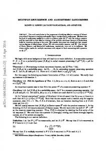
Figure 1. A hexagon. Note the absence of arithmetic progressions of length three. construction with

3

1 X a := id + (ei + e∗i ); 100 i=0 this is easily seen to be positive and self-adjoint, and a modification of the above computations then shows that 2 τ (aαn (a)α2n (a)α3n (a)) = 1 + 1A (n) 1004 for all n, which is enough to ensure divergence by choosing A appropriately. We leave the details to the reader. C Remark 2.3. The group G constructed here can easily be shown to have infinite conjugacy classes (by the same methods used to prove Proposition B.8). This implies that the group algebra LG is a factor. We refer to Kadison, Ringrose [26, Theorem 6.7.5] for details. C 2.2. Negative averages for k = 3. We now show the negativity of various triple averages. The main tool is the following Behrend-type construction of a set which avoids progressions of length three, but contains many “hexagons”: Lemma 2.2 (Behrend-type example). Let ε > 0. Then for all sufficiently large d, there exists a subset F of Z/dZ such that |F | ≥ d1−ε , but F contains no non-trivial arithmetic progressions of length three, thus n, n + r, n + 2r ∈ F can only occur if r = 0. On the other hand, the set {(x, h, k) ∈ Z/dZ : x, x + h, x + k, x + k + 2h, x + 2k + h, x + 2k + 2h ∈ F } of “hexagons” in F has cardinality at least d3−ε . We remark that the first part of the lemma already follows directly from the work of Behrend [2] or the earlier work of Salem and Spencer [33]. The claim about hexagons will be needed in the proof of Theorem 2.6 below, but is not needed for the simpler results in Corollary 2.4 or Theorem 2.5. Proof. Let R be a large multiple of 400 (depending on ε). We claim that for n a large enough multiple of 4 (depending on R), the set {−R, . . . , R}n ⊂ Zn contains

14


a subset E of cardinality |E| ≥ e−O(n) Rn (where the implied constant in the O() notation is absolute), and which contains ≥ e−O(n) R3n hexagons {x, x + h, x + k, x + k + 2h, x + 2k + h, x + 2k + 2h} but contains no arithmetic progressions of length three. Choosing d sufficiently large, letting n be the largest integer such that (10R)n ≤ d and then embedding {−R, . . . , R}n in Z/dZ using base 10R (say), as in the work of Behrend or Salem-Spencer, this claim will imply the lemma (choosing R sufficiently large depending on ε). It remains to establish the claim. From the classical results on the Waring problem (see e.g. [38]), we know that every large integer N has ∼ N (k−2)/2 representations as the sum of k squares for k large enough (one can for instance take k = 5, but for our purposes any fixed k will suffice). Using this, we see that for any 1 1 ), every integer r such that δR2 n ≤ r ≤ 10 R2 n (say) will have fixed δ ∈ (0, 10 n−Cδ ≥ (cδ R) representations as the sum of n squares of integers less than R, where cδ , Cδ > 0 depend only on δ. In other words, the sphere Er := {x ∈ {−R, . . . , R}n : |x|2 = r} has cardinality at least (cδ R)n−Cδ . On the other hand, such spheres have no non-trivial progressions of length three. Thus it will suffice (for n large enough) by the pigeonhole principle to show that there are at least e−O(n) R3n hexagons {x, x + h, x + k, x + k + 2h, x + 2k + h, x + 2k + 2h} in {−R, . . . , R}n such that 1 2 R n (9) |x|2 = |x+h|2 = |x+k|2 = |x+k+2h|2 = |x+2k+h|2 = |x+2k+2h|2 ≤ 10 (note that the case when |x|2 ≤ δR2 n for sufficiently small δ can be eliminated by crude estimates). To count the solutions to (9), we perform some elementary changes of variable to replace the constraints in (9) with simpler constraints. We begin by observing that if a, b, c ∈ {−R/100, . . . , R/100}n are such that (10)

a · b = b · c = c · a = 0;

c · c = 3b · b

then x := a − 2b, h := b + c, k := b − c can be verified to be a solution to (9), with the map (a, b, c) → (x, h, k) being injective, so it suffices to show that there are at least e−O(n) R3n triples (a, b, c) with the above properties. For reasons that will become clearer later, we will initially work in dimension n/4 rather than n. Using the Waring problem results as before, we can find at least e−O(n) R3n/4 triples a, b, c ∈ {−R/400, . . . , R/400}n/4 such that c · c = 3b · b. This is one of the four constraints required for (10). To obtain the remaining constraints, we use a pigeonholing trick followed by a tensor power trick. Firstly, observe that whenever a, b, c ∈ {−R/400, . . . , R/400}n/4 , then a·b, b·c, c·a are of order O(R2 n) ≤ eO(n) . Applying the pigeonhole principle, one can thus find h1 , h2 , h3 = O(R2 n) such that there are e−O(n) R3n/4 triples a, b, c ∈ {−R/400, . . . , R/400}n/4 with (11)

a · b = h1 ;

b · c = h2 ;

c · a = h3 ;

c · c = 3b · b.

This is an inhomogeneous version of (10) (at dimension n/4 rather than n), with the zero coefficients replaced by more general coefficients h1 , h2 , h3 . To eliminate these coefficients we use a tensor power trick. Let S ⊂ {−R/400, . . . , R/400}n/4 × {−R/400, . . . , R/400}n/4 × {−R/400, . . . , R/400}n/4 be the set of all triples (a, b, c)


15

obeying (11). We then observe that if (ai , bi , ci ) ∈ S for i = 1, 2, 3, 4, then the vectors a, b, c ∈ Zn defined by a := (a1 , a2 , a3 , a4 );

b := (b1 , b2 , −b3 , −b4 );

c := (c1 , −c2 , c3 , −c4 )

solve (10). The map from the (ai , bi , ci ) to (a, b, c) is an injection from S 4 to the solution set of (10), and so we obtain at least |S|4 ≥ e−O(n) R3n solutions to (10) as required. This leads to a useful matrix counterexample: Lemma 2.3 (Restricted third moment can be negative). There exists a positive semi-definite Hermitian matrix (A(j, k))1≤j,k≤d for which the quantity X (12) A(n, n + r)A(n + r, n + 2r)A(n + 2r, n) n,r∈Z/dZ

is negative, where we extend A(i, j) periodically in both variables by d. Proof. We will take d to be a multiple of 3, and A(j, k) to take the form A(j, k) := 1E (j)1E (k) + 1E (j)ω −j 1E (k)ω k where E ⊂ Z/dZ is a set to be determined later, and ω := e2πi/3 is a cube root of unity. The matrix (A(j, k))1≤j,k≤d is then the sum of two rank one projections and is thus positive semi-definite and Hermitian. The expression (12) can be expanded as X (1 + ω r )(1 + ω r )(1 + ω −2r ). n,r∈Z/dZ:n,n+r,n+2r∈E

The summand can be computed to equal 8 when r is divisible by 3, and −1 otherwise. Thus, to establish the claim, it suffices to find a set E such that the set {(n, r) ∈ Z/dZ : n, n + r, n + 2r ∈ E; r 6= 0 mod 3} is more than eight times larger than the set {(n, r) ∈ Z/dZ : n, n + r, n + 2r ∈ E; r = 0 mod 3}, thus the length three arithmetic progressions in E with spacing not divisible by 3 need to overwhelm the length three progressions with spacing divisible by 3. To do this, we use Lemma 2.2 to obtain a subset F ⊂ {1, . . . , [d/10]} of cardinality |F | ≥ d0.99 which contains no arithmetic progressions of length three. We then pick three random shifts h0 , h1 , h2 ∈ {1, . . . , d/3} uniformly at random, and consider the set E := {3(f + hi ) + i : i = 0, 1, 2; f ∈ F } consisting of three randomly shifted, dilated copies of F . By construction, the only length three progressions in E with spacing divisible by 3 are the trivial progressions n, n, n with r = 0, so the total number of such progressions is at most d. On the other hand, for any fixed f0 , f1 , f2 ∈ F , the numbers 3(fi + hi ) + i for i = 0, 1, 2 have a probability 3/d of forming an arithmetic progression with spacing not divisible by 3, due to the random nature of the hi . Thus the expected value of the total number of such progressions is at least (d0.99 )3 × 3/d = 3d1.97 . For d large enough, this gives the claim.

16


This already gives a simple example of negative averages for non-ergodic systems: Corollary 2.4 (Negative average for non-ergodic system). There exists a finite von Neumann algebra (M, τ ) with a shift α, and a non-negative element a ∈ M, PN such that 2N1+1 n=−N τ (aαn (a)α2n (a)) converges to a negative number. Proof. Let a = (A(j, k))1≤j,k≤d be as in Lemma 2.3. We let M be the von Neumann algebra of complex d × d matrices with the normalised trace τ , and with the shift α(B(j, k))1≤j,k≤d := (e2πi(j−k)/d B(j, k))1≤j,k≤d . This is easily verified to be a shift. We see that 1 X e2πin(k+l−2j)/d A(j, k)A(k, l)A(l, j). τ (aαn (a)α2n (a)) = d j,k,l∈Z/dZ

This expression is periodic in n with period d, and has average 1 X A(l, l + r)A(l + r, l + 2r)A(l + 2r, l) d l,r∈Z/dZ

and the claim then follows from Lemma 2.3.

This shows that recurrence on average for k = 3 can fail for non-ergodic systems. However, this is not yet enough to establish either Theorem 1.11 or Theorem 1.12. To obtain these stronger results we must introduce the crossed product construction in von Neumann algebras. For a comprehensive introduction to this concept, see [26, Chapter 13]. We shall just recall the key properties of this construction we need here. Suppose we have a finite von Neumann algebra (M, τ ), and an action U of a (discrete) group G on M, thus for each g ∈ G we have a shift U (g) : M → M such that U (g)U (h) = U (gh) for all g, h ∈ G, with U (id) being the identity. Then there exists a crossed product (MoU G, τ ) which contains both the original space (M, τ ) and the group algebra CG as subalgebras. Furthermore, in this crossed product we have U (g)a = gag −1

(13) for all a ∈ M and g ∈ G, and

τ (ga) = τ (ag) = 0 for all a ∈ M and g ∈ G with g not equal to the identity. Finally, the span of the elements ag for a ∈ M and g ∈ G is dense in M oU G. Remark 2.4. The exact construction of the crossed product is not relevant for our applications, but for the convenience of the reader we sketch one such construction here. We first form the Hilbert space M h := `2 (G, L2 (τ )) = L2 (τ ) g∈G

consisting of tuples (xg )g∈G in L2 (τ ). This space has an action of M defined by a(xg )g∈G := ((U (g −1 )a)xg )g∈G


17

for a ∈ M, and an action of G (and hence CG) defined by h(xg )g∈G := (xh−1 g )g∈G . One can verify that these actions combine to an action of the twisted convoluP 1 tion algebra ` (G, M) on h, defined as the space of formal sums ha h with h∈G P ka k < ∞, and subject to the relations (13). We define a trace on such sums h h∈G P by the formula τ ( h∈G hah ) := τ (aid ). One can then show that one can extend this to a finite trace on the weak operator topology closure of `1 (G, M), viewed as a subset of B(h); this closure can then be denoted M oU G. In other words, M oU G is constructed as the von Neumann algebra generated by the action of M and G on h. C Example 2.5. The group von Neumann algebra LG can be viewed as C o G, where G acts trivially on the one-dimensional von Neumann algebra C. C We can now get a stronger version of Corollary 2.4: Theorem 2.5 (Negative trace for non-ergodic system). There exists a von Neumann dynamical system (M, τ, α) and a non-negative element a ∈ M, such that τ (aαn (a)α2n (a)) is negative (and independent of n) for all non-zero n. In particular, Theorem 1.12 holds. Proof. Let (M0 , τ, β) be a von Neumann dynamical system to be chosen later. Using the crossed product construction, we can build an extension M := M0 oU Z2 of M0 generated by M0 and two commuting unitary elements u, m, such that mam−1 = β(a)

(14) and

uau−1 = a for all a ∈ M0 . In particular, the element u is central. It is then easy to see that we can build4 a shift α on M for which α(a) = a;

α(u) = u;

α(m) = mu

0

for all a ∈ M , since the action of the group Z2 generated by m and u on M0 is unchanged when one replaces m by mu. Now let a ∈ M be an element of the form ! !∗ X X i i a= fi m fi m i∈Z

i∈Z

0

where fi ∈ M , and only finitely many of the fi are non-zero. This is clearly non-negative, and can be simplified by (14) to the power series X a= gh mh h∈Z 4 space h := L To build2 α explicitly, we can view M as an algebra of operators on the Hilbert ∗ by the unitary L (τ ) as per Remark 2.4, and let α be the conjugation a → 7 W aW 2 (j,k)∈Z operator W : h → h defined by W (x(j,k) )(j,k)∈Z2 := (x(j,k−j) )(j,k)∈Z2 .

18


where the gh ∈ M0 are the twisted autocorrelations of the fj , X gh = fj+h β h (fj∗ ). j∈Z

Let n be non-zero. The expression τ (aαn (a)α2n (a)) can be expanded as X τ (gh1 mh1 gh2 (mun )h2 gh3 (mu2n )h3 ). h1 ,h2 ,h3 ∈Z

The net power of the central element u here is n(h2 +2h3 ), and the net power of m is h1 +h2 +h3 . Thus we see that the trace vanishes unless h2 +2h3 = h1 +h2 +h3 = 0, or equivalently if (h1 , h2 , h3 ) = (h, −2h, h) for some h. Performing this substitution and using (14), we simplify this expression to X (15) τ (gh β h (g−2h )β −h (gh )). h∈Z

In particular, this expression is now manifestly independent of n 6= 0. We now select M0 to be the commutative von Neumann system L∞ (Z/dZ) with the shift β(f (x)) := f (x + 1) and the normalised trace. Thus the gh and fh are now complex-valued functions on Z/dZ, and the above expression can be expanded explicitly as 1 X X gh (x)g−2h (x + h)gh (x − h). d x∈Z/dZ h∈Z

Meanwhile, the gh (x) by definition can be written as X gh (x) = fj+h (x)fj (x + h). j∈Z

We pick a large number N to be chosen later, and set fj (x) := b(x, x + j)11≤j≤N d where b : Z/dZ × Z/dZ → C is a function periodic in two variables of period d to be chosen later. Then we can compute |h| gh (x) = 1 − N A(x, x + h) + O(1) dN + where (16)

A(x, y) :=

X

b(x, z)b(y, z)

z∈Z/dZ

and O(1) denotes a quantity that can depend on d (and b) but is uniformly bounded in N . The expression (15) can then be computed to be C

N4 d

X

A(x, x + h)A(x + h, x − h)A(x − h, x) + O(N 3 )

x,h∈Z/dZ

where C > 0 is the explicit constant Z C := (1 − |h|)2+ (1 − |2h|)+ dh. R


19

By the substitution x = m + r, h = r, we can re-express this as N4 X (17) C A(m, m + r)A(m + r, m + 2r)A(m + 2r, m) + O(N 3 ). d m,r∈Z/dZ

Now, let d and A(j, k) be as in Lemma 2.3. By the spectral theorem (which in particular allows one to construct self-adjoint square roots of positive definite matrices), we can find b(x, y) so that (16) holds. The summand in (17) is then negative, and the claim follows by choosing N large enough depending on all other parameters. Of course, by Theorem 1.10, one cannot have such a result when the underlying shift α is ergodic. On the other hand, one can extend Corollary 2.4 to the ergodic case: Theorem 2.6. There exists an ergodic von Neumann system (M, τ, α) and a nonPN negative element a ∈ M, such that 2N1+1 n=−N τ (aαn (a)α2n (a)) converges to a negative number. In particular, Theorem 1.11 holds. Proof. Let d be a large odd number, and let u := e2πi/d be a primitive dth root of unity. We will let M be a completion of the non-commutative torus. This is obtained by first forming the C∗ -algebra generated by two unitary generators e1 , e2 obeying the commutation relation e2 e1 = ue1 e2 j k e1 e2 having zero

and with all of the expressions trace unless j = k = 0, in which case the trace is 1; and then completing in the weak operator topology resulting from the Gel’fand-Naimark-Segal representation on L2 (τ ). One can represent this finite von Neumann algebra more explicitly by letting e1 , e2 act on L2 ((R/Z)2 ) by the maps e1 f (x, y) := e2πix f (x, y) and e2 f (x, y) := e2πiy f (x + 1/d, y), with the trace τ given by τ (a) = hΩ, aΩiL2 ((R/Z)2 ) , where Ω ≡ 1 is the identity function on (R/Z)2 . We let θ1 , θ2 ∈ S 1 be generic unit phases, and then define the shift α on M by setting α(e1 ) := θ1 e1 ; α(e2 ) := θ2 e2 . It is easy to see that this is a shift. If θ1 , θ2 are generic (so that θ1j θ2k is not a root of unity for any (j, k) 6= (0, 0)), this shift is easily verified to be ergodic (as one can verify the mean ergodic theorem by hand on the generators ej1 ek2 , and then argue as in the proof of Theorem 2.1 using the faithfulness of τ ). We set a := gg ∗ , where g is an element of the form g :=

M X X

ch eh1 ek2 ,

k=1 h∈Z

M is a large number (much larger than d) to be chosen later, and ch are complex numbers to be chosen later, all but finitely many of which are zero. Clearly a is non-negative. A computation shows that X a= ch,k eh1 ek2 h,k∈Z

20


where (18)

1−

ch,k := M

|k| M

X

cl+h cl ukl .

+ l∈Z

Since αn (a) =

X

ch,k θ1hn θ2kn eh1 ek2 ,

h,k∈Z

some Fourier analysis and the genericity of θ1 , θ2 show that the expression N X 1 τ (aαn (a)α2n (a)) 2N + 1 n=−N

converges as N → ∞ to the expression X ch,k c−2h,−2k ch,k τ (eh1 ek2 e−2h e−2k eh1 ek2 ). 1 2 h,k

The trace here simplifies to u3hk . Inserting (18), we can expand this expression as X (19) M3 φ(k/M )cl1 +h cl1 cl2 −2h cl2 cl3 +h cl3 ukl1 −2kl2 +kl3 +3hk h,k,l1 ,l2 ,l3 ∈Z

where φ(x) := (1 − |x|)2+ (1 − |2x|)+ . By Poisson summation, the expression X φ(k/M )ukl1 −2kl2 +kl3 +3hk k

R

can be computed to be M R φ(x)dx + O(1) if l1 − 2l2 + l3 + 3h is divisible by d, and O(1) otherwise, where O(1) denotes a quantity that can depend on d but is bounded uniformly in M . If we then assume that the ch vanish for h outside of {1, . . . , M } and are bounded uniformly in M , we can thus expand (19) as X CM 4 cl1 +h cl1 cl2 −2h cl2 cl3 +h cl3 + O(M 7 ) h,l1 ,l2 ,l3 ∈Z: d|l1 −2l2 +l3 +3h

for some absolute constant C > 0. If we now set ch := b(h)1[1,M ] (h), where b : Z/dZ → C is a periodic function with period d and independent of M to be chosen later, we can express this as X Cd M 8 b(l1 +h)b(l1 )b(l2 −2h)b(l2 )b(l3 +h)b(l3 )+O(M 7 ) h,l1 ,l2 ,l3 ∈Z/dZ: l1 −2l2 +l3 +3h=0

for some Cd > 0 depending on d but independent of M . Making the substitution l1 = x; l2 = x + k + 2h; l3 = x + 2k + h, we see that we will be done as soon as we are able to find d, b for which the expression X X := b(x)b(x + h)b(x + k)b(x + k + 2h)b(x + 2k + h)b(x + 2k + 2h) x,h,k∈Z/dZ

is negative. To do this, we again appeal to Lemma 2.2 to find a set F ⊂ Z/dZ of size at least d0.99 (assuming d large enough), which contains no arithmetic progressions of length


21

three, but contains at least d2.99 hexagons x, x + h, x + k, x + k + 2h, x + 2k + h, x + 2k + 2h. We then set b(x) := x 1F (x) where the x = ±1 are independent signs, thus X is now the random variable X X= x x+h x+k x+2h+k x+h+2k x+2h+2k . x,h,k:x,x+h,x+k,x+k+2h,x+2k+h,x+2k+2h∈F

We will show (for d large enough) that the standard deviation of X exceeds its expectation, which shows that there exists a choice of signs for which X is negative. We first compute the expectation of X. The only summands with non-zero expectation occur when all the signs cancel, which only occurs when h = 0 or when k = 0, as can be seen by an inspection of the number of ways to collapse the hexagon in Figure 1; here we need the hypothesis that d is odd. But as F contains no non-trivial arithmetic progressions, there are no summands for which only one of the h, k are zero, so we are left only with the h = k = 0 terms, of which there are at most d. Thus the expectation of X is at most d. Now we compute the variance. There are at least d2.99 hexagons in F , and all but O(d2 ) of them are non-degenerate in the sense that the six vertices of the hexagon are all distinct. The summands in X corresponding to non-degenerate hexagons have variance 1, and the correlation between any two summands in X either zero or positive (the latter occurs when two summands are permutations of each other). Thus the variance of X is d2.99 , so the standard deviation is d1.495 , and the claim follows. 2.3. Negative trace for k = 5. Now we show negative traces can occur even in the ergodic case when k = 5. Theorem 2.7. There exists an ergodic von Neumann dynamical system (M, τ, α) and a non-negative element a ∈ M, such that τ (aαn (a)α2n (a)α3n (a)α4n (a)) is negative for every non-zero n. This establishes the k = 5 case of Theorem 1.13. A similar argument holds for all larger odd values of k, which we leave to the interested reader; we restrict here to the case k = 5 simply for ease of notation. To prove this theorem, our starting point is the following result of Bergelson, Host, Kra, and Ruzsa [4]: Theorem 2.8. For any δ > 0, there exists a measure-preserving system (X, X , µ, S) and a measurable set A ⊂ X with 0 < µ(A) < δ such that µ(A ∩ S n (A) ∩ S 2n (A) ∩ S 3n (A) ∩ S 4n (A)) ≤ µ(A)100 (say) and (20)

µ(A ∩ S n (A)) = µ(A)2

for every non-zero integer n. Proof. This follows from [4, Theorem 1.3] (see also the remark immediately below that theorem). The property (20) is not explicitly stated in that theorem, but

22


follows from the construction in [4, Section 2.3] (the system X is a torus (R/Z)2 with the skew shift S : (x, y) 7→ (x + α, y + 2x + α), and the set A has the special form A = (R/Z) × B for some set B). We apply this theorem for some sufficiently small δ (to be chosen later) to obtain X, µ, S, A with the above properties. We will combine this with the group G, the automorphism T , and the elements e0 , e1 , e2 , e3 , e4 arising from Proposition B.9 as follows. G First, we create the product space L∞ (XN , dµG ), whose σ-algebra is generated up to negligible sets by the tensor products g∈G fg , where fg ∈ L∞ (X, dµ) is equal to 1 for all but finitely many g. This product has a unitary, trace-preserving action U of G, defined by O O U (h) fg := fh−1 g . g∈G

g∈G

We can therefore create the crossed product M := L∞ (X G , dµG ) oU G. Note that if we embed L∞ (X, µ) into L∞ (X G , dµG ) by using the identity component of X G , we have O Y (21) fg = U (g)fg g∈G

g∈G

(note that the U (g)fg necessarily commute with each other.) We define a shift α on M by requiring that O O α( fg ) = S(fT −1 g ) g∈G

g∈G

and α(g) = T g; one can check that this is indeed a well-defined shift on M. We claim that α is ergodic. Indeed, if a ∈ M is of the form a = f g for some f ∈ L∞ (X G , dµG ) and g ∈ G not equal to the identity, then as the powers of T have no non-trivial fixed points, the orbit T n g escapes to infinity, and the orbit αn (a) converges weakly to zero. Meanwhile, if g is the identity, then it is classical that the Bernoulli system G L∞ (X G , dµG ) is ergodic, and so the ergodic theorem applies to a in this case. Putting the two facts together and arguing as for the ergodicity in Theorem 2.1 yields the ergodicity of α. Note that 1A lies in L∞ (X, dµ), and can thus be identified with an element of M by the previous embedding. We set a :=

3 X

1A · (2 − ei − e−1 i ) · 1A .

i=0

Clearly a is non-negative. Now let n be non-zero, and consider the expression (22)

τ (aαn (a)α2n (a)α3n (a)α4n (a)).

Expanding out a, we obtain a linear combination of terms of the form τ (1A g0 1A 1S n (A) (T n g1 )1S n (A) 1S 2n (A) (T 2n g2 )1S 2n (A) 1S 3n (A) (T 3n g3 )1S 3n (A) 1S 4n (A) (T 4n g4 )1S 4n (A) )


23

where −1 −1 −1 −1 g0 , g1 , g2 , g3 , g4 ∈ {id, e0 , e1 , e2 , e3 , e4 , e−1 0 , e1 , e2 , e3 , e4 }.

This trace vanishes unless (23)

g0 T n g1 T 2n g2 T 3n g3 T 4n g4 = id.

By Proposition B.9, we conclude that g0 , g1 , g2 , g3 , g4 are either all equal to the iden−1 −1 −1 −1 tity, or are a permutation of e0 , e1 , e2 , e3 , e4 , or are a permutation of e−1 0 , e1 , e2 , e3 , e4 . In the latter two cases, the contribution to (22) is either zero or negative (being negative the trace of the product of several non-negative elements in a commutative von Neumann algebra). Here we are using the fact that 5 is odd. Discarding all of these contributions except the one where gi,0 = ei,0 (which has a non-trivial contribution thanks to Proposition B.9), we conclude that (22) is at most 105 τ (1A 1S n (A) 1S 2n (A) 1S 3n (A) 1S 4n (A) ) − τ (1A e0 1A 1S n (A) e1 1S n (A) 1S 2n (A) e2 1S 2n (A) 1S 3n (A) e3 1S 3n (A) 1S 4n (A) e4 1S 4n (A) ). By Theorem 2.8, the first expression is at most 105 µ(A)100 . Now consider the second expression. By Proposition B.9, we see that the partial products e0 e1 . . . ei for i = 0, 1, 2, 3 are distinct. Using (21), we conclude that the trace here can be computed as µ(S 4n (A)∩A)µ(A∩S n (A))µ(S n (A)∩S 2n (A))µ(S 2n (A)∩S 3n (A))µ(S 3n (A)∩S 4n (A)), which by (20) is equal to µ(A)10 . Thus the expression (22) is at most 215 µ(A)100 − µ(A)10 , which is negative if the upper bound δ for µ(A) is chosen to be sufficiently small. This concludes the proof of Theorem 2.7. Remark 2.6. Given that the counterexample in Theorem 2.8 can be extended to any k ≥ 5, it seems reasonable to expect that Theorem 1.13 can be extended to all k ≥ 5 (not just the odd k), though we have not pursued this issue. On the other hand, the analogue of Theorem 2.8 fails for k = 4, as was shown in [4]. Because of this, the k = 4 case of Theorem 1.13 remains open; the construction given here does not work, but it is possible that some other construction would suffice instead. C 3. Inclusions of finite von Neumann dynamical systems In this section we quickly recall some fairly well-known constructions relating to von Neumann dynamical systems and their basic properties, culminating in a treatment of Popa’s noncommutative version of the Furstenberg-Zimmer dichotomy from [32]. This material will be needed to establish the structure theorem (Theorem 1.9). Let (M, τ ) be a finite von Neumann algebra. As noted in the introduction, we can embed M into a Hilbert space L2 (τ ). In order to distinguish the algebra structure from the Hilbert space structure5, we shall refer in this section to the embedded 5It is tempting to ignore these distinctions and identify M c with M. While this is normally qutie a harmless identification, we will take some care here because we will be studying the bimodule action of M on L2 (τ ), and keeping track of this action can become notationally confusing if the algebra elements are identified with the vectors that they act on.

24


copy of an element a ∈ M of the algebra in L2 (τ ) as b a rather than a, thus for c = {b instance M a : a ∈ M} is a dense subspace of L2 (τ ). Clearly, L2 (τ ) has the structure of an M-bimodule, formed by extending the regular bimodule structure on M by density; the left-representation is, of course, the classical Gel’fand-Naimark-Segal representation associated to τ . When it is necessary to denote the copy of M in B(L2 (τ )) consisting of the members of M acting by multiplication on the left (respectively, right), we will denote this algebra by Mleft (respectively, Mright ). The space L2 (τ ) contains a distinguished vector b 1 – the representative of the multiplicative identity 1 in M – with the property that ab 1=b 1a = b a for all a ∈ M. This vector will play a prominent role in the rest of this section. Now let (N , τ |N ) be a von Neumann subalgebra of (M, τ ) (with the inherited trace). Then we can canonically identify L2 (τ |N ) with the closed subspace 1N {bb : b ∈ N } = N b 1=b of L2 (τ ) in the obvious manner. We will make use of certain well-known properties of these constructs, which we merely recall here. A clear account of all of them can be found in [24, Chapters 1,3]. First, it is important that there is a simple necessary and sufficient condition for a c this is so if and only if the linear vector ξ ∈ L2 (τ ) to lie in the dense subspace M: operator c → L2 (τ ) : x M b 7→ xξ is bounded for the norm k · kL2 (τ ) , and so extends by continuity to a bounded operator L2 (τ ) → L2 (τ ). The necessity of this conclusion is clear, and its sufficiency requires just a little argument using the fact that for a finite von Neumann algebra (M, τ ) we have Mright = M00right and Mleft = M00left ; see [24, Theorem 1.2.4]. A simple application of this condition now shows that the orthogonal projection c into N b , and so defines also a linear eN : L2 (τ ) → N b 1 maps the dense subspace M operator EN : M → N . Indeed, for a ∈ M we need only to show that the map c → L2 (τ ) : x M b 7→ xeN (b a) is bounded for the norm k · kL2 (τ ) . Since N is also a von Neumann algebra and eN (b a) ∈ N b 1∼ = L2 (τ |N ), it actually suffices to check this for x ∈ N . However, since Nb 1 is an (N , N )-sub-bimodule, left multiplication by x commutes with eN , and so we have kxeN (b a)kL2 (τ ) = keN (xb a)kL2 (τ ) ≤ kc xakL2 (τ ) ≤ kakkb xkL2 (τ ) , as required. The linear operator EN is referred to as the conditional expectation of M onto N associated to τ , and it has the following readily-verified properties: Lemma 3.1 (Properties of conditional expectation). For all a ∈ M, the operator EN satisfies:


• • • • •

25

(Idempotence) EN (EN (a)) = EN (a); (Contractivity) kEN (a)k ≤ kak; (Trace-preservation) τ |N (EN (a)) = τ (a); (Positivity) EN (a∗ a) ≥ 0 (as a member of N ); and (Relation with eN ) For all ξ ∈ L2 (τ ), one has eN (a(eN (ξ))) = EN (a)(eN (ξ)) = eN (EN (a)(ξ)).

Example 3.1. If M = L∞ (X, X , µ) for some probability measure µ with the usual trace, and (Y, Y, ν) is a factor space of (X, X , µ) with a measurable factor map π : X → Y that pushes µ forward to ν, then L∞ (Y, Y, ν) can be identified with a subalgebra of M, and the conditional expectation map becomes its classical counterpart from probability theory. C Together with M, the orthogonal projection eN now generates in B(L2 (τ )) a larger von Neumann algebra hM, eN i ⊇ M. In general hM, eN i is no longer a finite von Neumann algebra, but it does contain the dense ∗-subalgebra A := lin(M∪{xeN y : x, y ∈ M}) on which we define the lifted trace τ¯ : A → C by specifying τ¯(xeN y) = τ (xy). By choosing an orthonormal basis for L2 (τ ) relative to the right action of N , and consequently realizing hM, eN i as an amplification of N , this linear map is seen to be non-negative and faithful, and hence defines a semifinite normal faithful [0, +∞]-valued trace (which we still denote by τ¯) on the cone (hM, eN i)+ of nonnegative (and self-adjoint) elements of hM, eN i. This witnesses that the algebra hM, eN i is semifinite (that is, any positive element of it may be approximated from below by finite-¯ τ positive elements). We will not spell out these standard manipulations here (see, for instance, [32, Section 1.5]), but we will invoke a notion of orthonormal basis for right-N -submodules of L2 (τ ) shortly. Remark 3.2. In case N ⊂ M is a finite-index inclusion of finite II1 factors, then we find that hM, eN i is also a finite II1 factor. Writing M1 for this factor, it follows that the above construction may be repeated with the inclusion M ,→ M1 in place of N ,→ M, and indeed that it may be iterated to form an infinite tower of II1 factors N ⊂ M ⊂ M1 ⊂ M2 ⊂ . . . . This is Jones’ basic construction; it underlies his famous work [25] on the possible values of the index [N : M], and also several more recent developments. Once again we refer the reader to [24] for a thorough account of its importance, and numerous further references. However, since the construction of this whole infinite tower is special to the case of II1 factors, we will not focus on it further here. C It is easy to check that the right action of any n ∈ N commutes with any xeN y, and hence with any member of hM, eN i, and in fact it can be shown that hM, eN i0 = 0 Nright and hence that Nright = hM, eN i00 = hM, eN i: firstly, if A ∈ B(L2 (τ )) commutes with every b ∈ Mleft then it must be the right-action of some a ∈ M, and now if also eN (b 1a) = b 1a then we must in fact have a ∈ N (see Proposition 3.1.2 in [24]). Let us record the following immediate but important consequence of this for our later work: Lemma 3.2. If V ≤ L2 (τ ) is a closed right-N -submodule, then the orthogonal projection PV : L2 (τ ) → V is a member of hM, eN i.

26


Using τ¯ we can also define an alternative completion of A = lin MeN M for each p p ∈ [1, ∞) by setting kAkp,¯τ := p τ¯((A∗ A)p/2 ) for A ∈ A (where as usual the power (A∗ A)p/2 is defined using spectral theory for the selfadjoint operator A∗ A, and the non-negativity of τ¯ is used to show that τ¯((A∗ A)p/2 ) is finite even when p/2 is not an integer). We denote this completion by Lp (¯ τ ); it is a Hilbert space when p = 2. In general elements of Lp (¯ τ ) do not correspond to elements of hM, eN i, but they do give possibly unbounded but closable operators that are weakly approximable by members of this algebra, which are therefore affiliated to Nright . If A ∈ Lp (¯ τ ) is such an operator that is self-adjoint, then it admits a spectral decomposition Z A= s P (ds) R

for some spectral measure P on R taking values in the projections of hM, eN i ∩ L1 (¯ τ ), of possibly unbounded support in R, but for which Z kAkpp,¯τ = |s|p τ¯P (ds) < ∞. R

If V is as in Lemma 3.2 then we may write that PV has finite lifted trace if it corresponds to a member of hM, eN i ∩ L1 (¯ τ ). Now let us introduce some dynamics. Suppose that α is a shift on M which restricts to a shift on N . Then, as mentioned in the introduction, α induces a unitary operator acting on L2 (τ ), which we shall distinguish from α by writing it as Uα ; thus for instance d Uα b a = Uα (ab 1) = α(a)b 1 = α(a) 1 is an invariant subspace for Uα , so that Uα for all a ∈ M. It is clear that N b commutes with eN . Also, conjugation by Uα agrees with the action α on M, thus Uα aUα−1 ξ = α(a)ξ for all a ∈ M and ξ ∈ L2 (τ ). Thus, conjugation by Uα extends the action of α to hM, eN i. The following special class of one-sided submodules of L2 (τ ) appears here almost exactly as in the commutative setting. Definition 3.3 (Finite-rank modules). A left- (respectively, right-) N -submodule V of L2 (τ ) has finite rank if there are some ξ1 , ξ2 , . . . , ξr ∈ V such that V = Pr Pr i=1 N ξi (respectively, V = i=1 ξi N ), and the numerical value of its rank is the least r ≥ 1 for which this is possible. Proposition 3.4 (Relativized Gram-Schmidt procedure). If V ≤ L2 (τ ) is a Uα invariant right-N -submodule of finite rank r then there are ξ1 , ξ2 , . . . , ξr ∈ L2 (τ ) such that • the subspaces ξi N ≤ L2 (τ ) are pairwise orthogonal; and Pr • V = i=1 ξi N . Proof. This uses a relativized Gram-Schmidt argument much as in the commutative setting (see e.g. [18, Lemma 9.4]). We proceed by induction on r. If V has rank 1


27

then the result is immediate from the definition, so let us suppose that it has rank r + 1 for some r ≥ 1. Then given a representation V =

r+1 X

ξi◦ N ,

i=1

we know that any member of V may be approximated in k · kL2 (τ ) by expressions ◦ of the form ξ1◦ n1 + · · · + ξr+1 nr+1 for n1 , n2 , . . . , nr+1 ∈ N . This, in turn, may be re-written as ◦ (ξ1⊥ n1 + · · · + ξr⊥ nr ) + (ξ1◦ − ξ1⊥ )n1 + · · · + (ξr◦ − ξr⊥ )nr + ξr+1 nr+1 where for each i ≤ r we have decomposed ξi◦ into its component ξi⊥ orthogonal to ξr+1 N and the remainder ξi◦ − ξi⊥ ∈ ξr+1 N . Since ξr+1 N is a right-N -submodule, it follows that the second and third inner sums in the above decomposition both ⊥ lie in ξr+1 N , and now since ξr+1 N is also a right-N -submodule, we have in fact shown that V = V1 + ξr+1 N Pr

where V1 := i=1 ξi⊥ N is a rank-r right-N -submodule that is orthogonal to ξr+1 N . Applying the inductive hypothesis to V1 now completes the proof. The following definition is also drawn from the commutative world. This notion has previously been extended to the setting of non-commutative algebras by Popa in [32], who discusses several other aspects and equivalent conditions in that paper. (See also [31], [11], [6] for an analysis of the absolute analogue of weak mixing, in which the subalgebra N is the trivial algebra C1.) Definition 3.5 (Relative weak mixing). If (M, τ, α) is a von Neumann dynamical system and N ⊂ M is an α-invariant von Neumann subalgebra, then α is weakly mixing relative to N if for any a ∈ M ∩ N ⊥ we have N 1 X kEN (a∗ αn (a))k2τ → 0 N n=1

as N → ∞.

The basic inverse theorem that we need, extending the idea of Furstenberg and Zimmer to the non-commutative context, is contained in the following proposition, which essentially re-proves part of [32, Lemma 2.10]: Proposition 3.6 (Lack of weak mixing implies finite trace submodule). If α is not weakly mixing relative to N then there is a Uα -invariant right-N -submodule 1 such that PV has finite lifted trace. V ≤ L2 (τ ) N b Proof. Suppose that a ∈ M ∩ N ⊥ is such that N 1 X kEN (a∗ αn (a))k2τ 6→ 0. N n=1

28


Define b := aeN a∗ ∈ hM, eN i, and now observe (using the cyclic permutability of τ¯ and the identity eN meN ≡ EN (m)eN ) that for any n ∈ N we have τ¯ b(Uαn bUα−n ) = τ¯(aeN a∗ Uαn (aeN a∗ )Uα−n ) = τ¯(aeN a∗ αn (a)eN αn (a)∗ ) = τ¯ EN (a∗ αn (a))eN αn (a)∗ a = kEN (a∗ αn (a))k2τ . Averaging in n it follows that N 1 X τ¯ b αn (b) → hb, b1 iτ¯ 6= 0 N n=1 PN where b1 is the limit of the ergodic averages N1 n=1 αn (b) in the Hilbertian completion L2 (¯ τ ), which is therefore invariant under the further extension of the unitary operator Uα to this Hilbert space.

This new element b1 need not, in general, correspond to a member of hM, eN i (it is easily seen to be so in the commutative setting, but for special reasons); however, 0 as a k · k2,¯τ -limit of members of hM, eN i = Nright it can always be identified with 2 a closed operator on L (τ ) that is affiliated with the right action of the algebra N , and as such it admits a spectral decomposition Z ∞ b1 = s P (ds) 0

for some resolution of the identity P on [0, ∞) whose contributing spectral projections lie in hM, eN i, and for which Z ∞ s2 τ¯(P (ds)) = kb1 k22,¯τ < ∞. 0

Hence τ¯P (I) < ∞ for any Borel subset I ⊆ (0, ∞) bounded away from 0. Now choosing any such subset I for which P (I) 6= 0 gives an orthogonal projection P (I) ∈ hM, eN i of finite lifted trace that is Uα -invariant, commutes with the rightN -action because it lies in hM, eN i, and moreover has image orthogonal to b 1N because we initially chose b to lie in the orthogonal complement of this subspace. Remark 3.3. The above implication can in fact be reversed, and these conditions shown to be equivalent to a number of others; see [32, Lemma 2.10] for a more complete picture. C In the next section we will push the above results a little further under the additional assumption that the subalgebra N is central, leading to the proof of Theorem 1.9. 4. The case of asymptotically abelian systems We now specialize to the case of an asymptotically abelian system, with the crucial additional assumption that the subalgebra N is central. Lemma 4.1. Suppose that (M, τ, α) is a von Neumann dynamical system, N ⊂ M is an α-invariant central von Neumann subalgebra and V ≤ L2 (τ ) is a Uα -invariant right-N -submodule of finite lifted trace. Then for any ε > 0 there is a further Uα invariant right-N -submodule V1 ≤ V such that


29

• τ¯(PV − PV1 ) < ε; • V1 has finite rank, say r ≥ 1; • there are an orthogonal right-N -basis ξ1 , ξ2 , . . . , ξr and a unitary matrix of unitary operators U = (uji )1≤i,j≤r ∈ Ur×r (N ) such that Uα (ξi ) =

r X

ξj uji

∀i = 1, 2, . . . , r.

j=1

We refer to U as the cocycle representing the action of Uα on the basis elements ξi . Proof. We will prove this invoking the picture of the representation of N on L2 (τ ) as a direct integral coming from spectral theory. By the classical theory of direct integrals (see, for instance, [26, Chapter 14]), we can select • a standard Borel probability space (Y, ν); S • a Borel partition Y = n≥1 Yn ∪ Y∞ ; • a collection of Hilbert spaces Hn for n ∈ {1, 2, . . . , ∞} with dim(Hn ) = n; and • a unitary equivalence Z ⊕ Φ : L2 (τ ) → H := Hy ν(dy), Y

where we define Hy to be Hn when y ∈ Yn , such that N (acting on the right or left, since these agree for a central subalgebra of M) is identified with the algebra of functions L∞ (ν) acting by pointwise multiplication. Explicitly, if we denote elements of H as measurable sections ` v : Y → y∈Y Hy , then f ∈ L∞ (ν) acts on H by Mf (v)(y) := f (y)v(y). 1) we select a measurable section v0 ∈ H Moreover, in order to accommodate Φ(N b with kv0 (y)kHy ≡ 1, and now N b 1 is identified with {y 7→ f (y)v0 (y) : f ∈ L∞ (µ)}, so that the orthogonal projection ΦeN Φ−1 acts by ΦeN Φ−1 (v)(y) := hv(y), v0 (y)iHy · v0 (y). The larger algebra Mright is identified under Φ with a direct integral Z ⊕ My ν(dy), Y

so that elements of Φ(M) are expressed as measurable sections T : Y → acting by T v(y) := T (y)(v(y))

`

y∈Y

B(Hy )

and such that T (y) ∈ My ν-almost surely, where (My )y∈Y is a measurable field of finite von Neumann subalgebras of B(Hy ) for each of which the state My → C : T 7→ hv0 (y), T (v0 (y))iHy

30


is a faithful finite trace; overall we have Z τ (a) = hb 1, ab 1i = hv0 (y), Φ(a)(y)(v0 (y))iHy ν(dy) Y

for a ∈ M, and so in particular if n ∈ N then Φ(n) ∈ L∞ (µ) and τ (n) =

R

Φ(n) dν.

Given these data, for a, b ∈ M we can compute that Φ(aeN b)Φ−1 v(y) = hΦ(b)(y)(v(y)), v0 (y)i · Φ(a)(y)(v0 (y)) and Z τ¯(aeN b) = τ (ab) = hv0 (y), Φ(ab)(y)(v0 (y))iHy ν(dy) Y Z Z = hΦ(a∗ )(y)(v0 (y)), Φ(b)(y)(v0 (y))iHy ν(dy) = tr(Φ(aeN b)Φ−1 |Hy ) ν(dy). Y

Y

In this representation an N -submodule V ≤ L2 (τ ) corresponds to a subspace R⊕ Φ(V ) ≤ H of the form Y Vy ν(dy) for some measurable subfield of Hilbert spaces Vy ≤ Hy , and the above calculation now shows that Z τ¯(PV ) = dim(Vy ) ν(dy), Y

so PV has finite lifted trace if and only if the function y 7→ dim(Vy ) is ν-integrable. We can enhance this picture further by noting that since α preserves N it must correspond to some ν-preserving transformation S y Y , and that since it also preserves M and extends to a unitary operator on L2 (τ ) it must also preserve each of the cells Yn . Similarly, since V is Uα -invariant, the transformation S must preserve the function y 7→ deg(Vy ). It follows that the unitary operator ΦUα Φ−1òn L2 (τ ) is actually given by a measurable section of unitary operators Ψ : Y → y∈Y U(Hy ) such that ΦUα Φ−1 v(y) = Ψ(y)(v(S −1 y)). Now, since y 7→ deg(Vy ) is ν-integrable, for sufficiently large r ≥ 1 we know that Z deg(Vy ) ν(dy) < ε. {y∈Y : deg(Vy )>r}

Define Z

⊕

Z

⊕

Vy ν(dy) ⊕

W := {y∈Y : deg(Vy )≤r}

{0} ν(dy) {y∈Y : deg(Vy )>r}

and V1 := Φ−1 (W ). Clearly V1 is still a right-N -submodule that is Uα -invariant, and it clearly also has rank at most r (since it suffices to prove this for W , for which it follows by a relativized Gram-Schmidt construction of a fibrewise-orthonormal basis exactly as in the setting of commutative ergodic theory; see for instance [18, Lemma 9.4]). Also, we have Z τ¯(PV − PV1 ) = deg(Vy ) ν(dy) < ε. {y∈Y : deg(Vy )>r}

Finally, the selection of unitaries Ψ must preserve the field of subspaces Vy above the S-invariant set {y ∈ Y : deg(Vy ) = s} for each s ≤ r. Choosing an abstract


31

d-dimensional Euclidean space Wd for each d ≤ r and adjusting each fibre of W by a unitary in order to identify each Vy for which dim(Vy ) ≤ r with Wdim(Vy ) , we obtain a new representation of V1 as a right-N -submodule using these fibres Wd , so that the action of Uα is now described by a measurable family of unitaries Ψ0 (y) ∈ U(Wdim(Vy ) ). Picking an orthonormal basis for each Wd , writing these unitary operators as unitary matrices in terms of these bases, noting that their individual entries are now identified with elements of L∞ (µ) = Φ(N ) and carrying everything back to L2 (τ ) using Φ−1 gives the desired expression for Uα . Remark 4.1. Frustratingly, both the fact that a Uα -invariant V of finite lifted trace may be approximated by a Uα -invariant V1 of finite rank, and the fact that given such a module of finite rank the action of Uα on it may be described by a unitary element in U(Mr×r (N )), seem to be difficult to prove without the assumption that N is central and the resulting representation of the action of N on L2 (µ) as the multiplication action of some L∞ (ν) on a measurable field of Hilbert spaces. It would be interesting to settle this issue more generally: Question 4.2. Do these conclusions hold for a finite-lifted-trace invariant submodule corresponding to an arbitrary inclusion of finite von Neumann algebras with a trace-preserving automorphism? C Before moving on let us quickly note an important difference from the setting of abelian von Neumann algebras. Example 4.2. If M is abelian, then from commutative ergodic theory it is wellknown that all the intermediate Uα -invariant submodules V ≤ L2 (τ ) that have finite-rank over N together generate an intermediate subalgebra between N and M, and that this then corresponds to an intermediate measure-preserving system. We will see shortly that an analogous conclusion can sometimes be recovered in the asymptotically abelian setting, but it is certainly not true for general finite-rank submodules, even when the smaller algebra N is abelian. Consider, for example, the inclusion i : LZ ∼ = L∞ (mT ) ,→ LF2 corresponding to the embedding of Z as the cyclic subgroup aZ of the free group F2 = ha, bi. Here LG is the group von Neumann algebra of G, defined in Section 2.1. In this case we can identify L2 (τ ) as `2 (F2 ) and L2 (τ |N ) as the subspace spanned by {ξan }n∈Z . Now define α ∈ Aut LF2 simply by lifting the group automorphism of F2 that fixes a and maps b 7→ ba. Now the subspace V := lin{ξban : n ∈ Z} ≤ `2 (F2 ) is a Uα -invariant right N -module of rank one which is orthogonal to L2 (τ |N ). On the c ∩ V , we have αm (ξ 2 ) = αm (ξb2 ) = ξbam bam for m ∈ Z, other hand, although ξb ∈ M b and it is easy to see that these elements of M do not remain within any finite-rank right-N -submodule. It is true that if L2 (τ ) L2 (τ |N ) contains a finite-rank right-N -submodule V , then it also contains a finite-rank left-N -module in the form of J(V ), where J is the modular automorphism on V , defined by extending the conjugation map a 7→ a∗ c by density. The point is that it can happen that J(V ) ⊥ V , and that on M ≡ M all elements of J(V ) are weakly mixed by Uα : it is the right-module V , and no other, that serves as the obstruction to overall relative weak mixing coming from Theorem 1.8. C

32


We now introduce a useful technical concept. Definition 4.3 (Central vectors). A vector ξ ∈ L2 (τ ) is central if mξ = ξm for all m ∈ M. Lemma 4.4 (No non-obvious central vectors). The closure Z(M)b 1=b 1Z(M) is 2 equal to the set of all central vectors in L (τ ). Proof. Suppose that ξ ∈ L2 (τ ) is central. Define aξ : Mb 1 → L2 (τ ) by aξ (mb 1) := 2 ξm. This is a densely-defined linear operator on L (τ ), and it is closable because if mnb 1=b 1mn → 0 in k · kL2 (τ ) for some sequence (mn )n≥1 in M and also ξmn → ξ 0 in k · kL2 (τ ) , then we have 1, ξmn i = lim hb 1m∗n , (m0 )∗ ξi = 0 1, ξ 0 i = lim hm0b hm0b n→∞

n→∞

0

for every m ∈ M, and so in fact we must have ξ 0 = 0. Also, we clearly have aξ (mb 1) = aξ (b 1m) = ξm = mξ = (aξ (b 1))m = m(aξ (b 1)) for every m ∈ M, so aξ is affiliated with both the right- and left-actions of M on L2 (τ ). The same therefore holds for aξ + a∗ξ and i(aξ − a∗ξ ), and now these are selfadjoint and so each of them may be expressed as an unbounded spectral integral all of whose contributing spectral projections must lie in M0left ∩ M0right = Z(M). Therefore, approximating aξ = 21 (aξ + a∗ξ ) + 12 (aξ − a∗ξ ) by a sum of two large but bounded integrals with respect to the respective resolutions of the identity, we obtain a sequence of elements an ∈ Z(M) such that an → aξ pointwise on dom(clos(aξ )) ⊇ Mb 1, and hence such that anb 1 → ξ in k · kL2 (τ ) . Hence ξ ∈ Z(M)b 1, as required. Proposition 4.5. If (M, τ, α) is an asymptotically abelian von Neumann dynamical system, N is a shift-invariant central von Neumann subalgebra, and V ≤ L2 (τ ) is an α-invariant right-N -submodule of M having finite lifted trace then all elements of V are central vectors. Proof. Clearly it will suffice to prove this for all finite-rank approximants V1 to V as given by Lemma 4.1. Thus we may assume that V actually has finite rank. Let ξ1 , ξ2 , . . . , ξr and U = (uji )1≤i,j≤r ∈ Mr×r (N ) be as given by the third part of that lemma. Since α is asymptotically abelian, we have for any ab 1 ∈ Mb 1 and b ∈ M that N N 1 X 1 X kbUαn (ab 1) − Uαn (ab 1)bkL2 (τ ) = kbαn (a) − αn (a)bkL2 (τ ) → 0. N n=1 N n=1

Approximating an arbitrary ξ ∈ L2 (τ ) by elements of Mb 1, it follows that for each fixed b ∈ M and ξ ∈ L2 (τ ) we have N 1 X kbUαn (ξ) − Uαn (ξ)bkL2 (τ ) = 0. N →∞ N n=1

lim


33

On the other hand, we know that Uα (ξi ) =

r X

∀i = 1, 2, . . . , r,

ξj uji

j=1 (n)

and so, writing U n = (uji )1≤i,j≤r , we have Uα−n (ξi ) =

r X

(−n)

ξj uji

j=1

⇒

ξi =

r X

(−n)

Uαn (ξj )αn (uji

)

∀i = 1, 2, . . . , r.

j=1

(−n)

Clearly each uji is still a unitary, and so from this, averaging in n and the centrality of N we obtain kbξi − ξi bkL2 (τ )

=

N X r r

1 X X

(−n) n n (−n) bUα (ξj )α (uji ) − Uαn (ξj )αn (uji )b 2

N n=1 j=1 L (τ ) j=1

=

N X r

1 X

(−n) bUαn (ξj ) − Uαn (ξj )b αn (uji ) 2

N n=1 j=1 L (τ )

≤

N r X 1 X kbUαn (ξj ) − Uαn (ξj )bkL2 (τ ) , N n=1 j=1

and now since each of the summands in j tends to 0 as N → ∞, it follows that we must in fact have bξi = ξi b for every i ≤ r, and hence (taking N -linear combinations, which have central coefficients, and then a completion) that all vectors in V are central, as required. Let us note explicitly the following simple corollary of the above result. Corollary 4.6. If (M, τ, α) is an asymptotically abelian von Neumann dynamical system, then the subalgebra Mα := {a ∈ M : α(a) = a} of individually α-invariant elements is central. Proof. Of course, if α(a) = a then lin{b 1a} is a rank-one α-invariant submodule 2 of L (τ ) for the trivial central subalgebra N := Cb 1, and the claim follows from Proposition 4.5. This claim can also be easily verified directly from the definition of asymptotic abelianness. Finally we can use the above results to prove Theorem 1.9. Proof. (Proof of Theorem 1.9) Suppose, for the sake of contradiction, that α were not weakly mixing relative to Z(M) ⊂ M. Then Proposition 3.6 gives a nontrivial right-Z(M)-submodule V ≤ L2 (τ ) Z(M)b 1 of finite lifted trace, and now Proposition 4.5 tells us that V must consist of central vectors. However, Lemma 4.4 now gives V ≤ Z(M)b 1, implying a contradiction with our assumption b that V ⊥ Z(M)1.

34


Note that for the results in this section it suffices to assume that for every a ∈ M there exists a sequence {nj } such that limj→∞ k[αnj (a), b]kL2 (τ ) = 0 for every b ∈ M. We do not know whether this condition is strictly weaker than asymptotically abelianness. Remark 4.3. A variant of Theorem 1.9 can also be deduced from the results in [31] (and more specifically, Theorem 4.2 and Proposition 5.5 of that paper); we thank the anonymous referee for pointing out this fact. More specifically, the result is that if α is an automorphism of a finite von Neumann algebra M that leaves invariant a faithful normal trace τ , and Eτ is the conditional expectation to the factor wot

Mr := lin

{a ∈ M : α(a) = λa for some λ ∈ T},

then for any a, b ∈ M one has N 1 X |hEτ (a∗ αn (a)) − Eτ (a)∗ αn (Eτ (a)), biL2 (τ ) | = 0; N →∞ N n=1

lim

in particular, for N going to infinity along a density one set of integers, the expression Eτ (a∗ αn (a)) − Eτ (a)∗ αn (Eτ (a)) converges to zero in the weak operator topology. This property is weaker than the relative weak mixing property with respect to this factor (which one does not expect to hold in general, even in the abelian case), but on the other hand does not require any hypothesis of asymptotic abelianness. 5. Triple averages for non-asymptotically-abelian systems The use to which we put relative weak mixing in the preceding section is very special to asymptotically abelian systems: in general there seems to be no way to track the error term resulting from the re-arrangement at the heart of the proof of Theorem 1.8 without this assumption. However, in the special case of triple averages this problem does simplify somewhat, provided we assume instead that our system (M, τ, α) is ergodic, so that Mα = C1. In this case we will be able to obtain convergence weakly and in norm, as well as recurrence on a dense set (Theorem 1.10). This assumption is not so innocuous as might be expected from its analog in the world of commutative ergodic theory. In that setting it is possible quite generally to decompose a system (that is, more precisely, to decompose its invariant measure) into ergodic components, and then many assertions about the whole system, including multiple recurrence and the convergence of multiple averages, follow if they can be proved for each ergodic component separately. However, in the setting of a general von Neumann dynamical system, this decomposition is available only if Mα is central in M; otherwise the automorphism α can exhibit genuinely new phenomena precisely in virtue of having the nontrivial fixed subalgebra Mα to ‘move around’. This was already seen in the failure of recurrence on a dense set when the ergodicity hypothesis is dropped (Theorem 1.12). The key for convergence of triple averages is the following decomposition similar to the commutative case, first established (in a slightly more general setting) in [31] (and more specifically, from Theorem 4.2 and Proposition 5.5 in that paper);


35

for the convenience of the reader we give a short proof of that decomposition here. Note that the result does not require ergodicity of the system. We remark that a closely related decomposition was also used in [13]. Proposition 5.1 (Decomposition of von Neumann dynamical systems). [31] Let (M, τ, α) be a von Neumann dynamical system. Then one has the orthogonal decomposition M = Mr ⊕ Ms , where Mr Ms

wot

:= lin ( :=

{a ∈ M : α(a) = λa for some λ ∈ T} and

N 1 X a ∈ M : lim |τ (b αn (a))| = 0 N →∞ N n=1

) for every b ∈ M ,

i.e., Mr is the von Neumann subalgebra spanned by the eigenvectors of α and Ms is the subspace of the elements of M that are weakly mixed by α. The corresponding projection onto Mr is the conditional expectation of M onto Mr and in particular preserves positivity. Proof. Since the continuation Uα of α to L2 (τ ) is a unitary operator, the Jacobs– Glicksberg–de Leeuw decomposition holds for Uα (see e.g. [29, Section 2.4]), i.e., L2 (τ ) = L2r (τ ) ⊕ L2s (τ ), where the reversible part L2r (τ ) is defined as L2r (τ ) = lin{x : Uα (x) = λx for some λ ∈ T} and the stable part L2s (τ ) is defined as the space of all x ∈ L2 (τ ) such that N 1 X |hUαn (x), yi| = 0 N →∞ N n=1

lim

for every y ∈ L2 (τ ).

Moreover, this decomposition is orthogonal since Uα is unitary. Note that we do not need here the Jacobs–Glicksberg–de Leeuw decomposition in full generality but only its version for unitary operators, which can be also proved via the spectral theorem. By a result of Størmer [34], the eigenvectors of Uα belong to M. We thus have Mr = M ∩ L2r (τ ) and Ms = M ∩ L2s (τ ). The fact that the weak operator closure and the closure in the L2 (τ )-topology coincide for self-adjoint subalgebras implies the second formula for Mr and thus Mr is a von Neumann subalgebra of M. The conditional expectation now maps M onto Mr assuring the orthogonal decomposition M = Mr ⊕ Ms . In the remainder of this section we assume our system is ergodic. Proposition 5.2 (Convergence of triple averages). Let (M, τ, α) be an ergodic von Neumann dynamical system. Then the averages (24)

N 1 X n α (a) α2n (b) N n=1

converge in k · kL2 (τ ) as N → ∞ for every a, b ∈ M.

36


Proof. By the above proposition, it suffices to assume that a and b each belong to Mr or Ms . Suppose first that a ∈ Mr , and fix b. The operators SN given by SN x =

N 1 X n α (x) α2n (b) N n=1

are linear and bounded on M for the norm k · kL2 (τ ) , so we may assume that PN α(a) = λa for some λ ∈ T. Then SN a = N1+1 n=0 a(λα2 )n (b) which converges in L2 (τ ) by the mean ergodic theorem. Suppose now that a ∈ Ms . We show that the desired limit is zero. Consider un := αn (a) α2n (b) b 1 and observe that hun , un+j i = τ (α2n (b∗ ) αn (a∗ ) αn+j (a) α2n+2j (b)) =

τ (αn (b∗ ) a∗ αj (a) αn+2j (b)) = τ (a∗ αj (a) αn (α2j (b) b∗ )).

The ergodicity of the system implies N 1 X γj := lim hun , un+j i N →∞ N n=1 ! N X 1 = τ a∗ αj (a) lim αn (α2j (b) b∗ ) = |τ (a∗ αj (a))| · |τ (α2j (b) b∗ )|. N →∞ N n=1 Since a ∈ Ms and τ (α2j (b) b∗ ) are bounded in j, we have N 1 X lim γj = 0, N →∞ N j=1

and therefore by the classical van der Corput lemma for Hilbert spaces (see e.g. PN [15] or [3]), we have limN →∞ N1 n=1 un = 0. Remarks 5.1. (1) For compact non-ergodic systems the averages (24) converge as well, since M = Mr in this case; this was also observed in [6]. (2) As in the commutative case we see that the Kronecker subalgebra Mr is characteristic for (24), i.e., the limit of the averages in (24) does not change if replacing a by EMr a and b by EMr b. C As was shown in Corollary 2.4, one cannot expect the limit N 1 X τ (aαn (a)α2n (a)) N →∞ N n=1

lim

to be positive for every positive a. However, a modification extending [6, Theorem 5.13] is still true. Proposition 5.3. For an ergodic von Neumann system (M, τ, α), one has lim inf N →∞

N 1 X (Re τ (a αn (a) α2n (a)))+ > 0 N n=1

for every 0 < a ∈ M. In particular, one has recurrence on a dense set.


37

Proof. Decompose a = b + c with b ∈ Mr and c ∈ Ms as in Proposition 5.1, with b > 0 by Lemma 3.1. We first show that there exists a compact abelian group G, an open set U ⊂ G and g ∈ G such that for the 1-step Bohr set KU := {n ∈ N : g n ∈ U } one has Re τ (b αn (b) α2n (b)) >

(25)

τ (b3 ) >0 2

for every n ∈ KU .

3

τ (b ) Take ε := 18kbk 2 . Since b ∈ Mr , we find k ∈ N, λ1 , . . . λk ∈ T and b1 , . . . , bk ∈ M \ {0} such that α(bj ) = λj bj for every j = 1, . . . , k and kb − (b1 + . . . + bk )kL2 (τ ) < ε. Set now G := Tk , g := (λ1 , . . . , λk ) and U := Uε/(k max kbj k) (1) ⊂ Tk . Observe that for every n such that g n ∈ U , we have |λnj − 1| < ε/(k max kbj k) for every j = 1, . . . , k and therefore

kαn (b) − bkL2 (τ )

kan (b1 + . . . + bk ) − (b1 + . . . + bk )kL2 (τ )

≤

+2kb1 + . . . + bk − bkL2 (τ ) max kbj kL2 (τ ) (|λn1 − 1| + . . . + |λnk − 1|) + 2ε kε max kbj k + 2ε = 3ε. k max kbj k

≤
0. N n=1

Next, we show that (27)

N 1 X f (g n )αn (b) α2n (c) = 0. N →∞ N n=1

k · kL2 (τ ) − lim

b and define To do this, we first consider a character γ ∈ G un := γ(g n )αn (b) α2n (c) b 1.

38


We have hun , un+j i = γ(g n )γ(g n+j )γ(α2n (c∗ ) αn (b∗ ) αn+j (b) α2n+2j (c)) = γ(g j )τ (αn (c∗ ) b∗ αj (b) αn+2j (c)) = γ(g j )τ (b∗ αj (b) αn (α2j (c) c∗ )). By ergodicity of α, N 1 X hun , un+j i = γ(g j )τ γj := lim N →∞ N n=1 =

! N X 1 b∗ αj (b) lim αn (α2j (c) c∗ ) N →∞ N n=1

|τ (b∗ αj (b))| · |τ (α2j (c) c∗ )|,

and the assumption c ∈ Ms implies limN →∞ Corput estimate we thus have

1 N

PN

j=1

γj = 0. By the van der

N N 1 X 1 X lim un = lim γ(g n )αn (b) α2n (c)b 1 = 0. N →∞ N N →∞ N n=1 n=1

Since the characters form a total set in C(G) and the operators SN f :=

N 1 X f (g n )αn (b) α2n (c) N n=1

are uniformly bounded on C(G), (27) is proved. Analogously one also has N N 1 X 1 X f (g n )αn (c) α2n (b) = k · kL2 (τ ) − lim f (g n )αn (c) α2n (c) = 0. N →∞ N N →∞ N n=1 n=1

k · kL2 (τ ) − lim

The Cauchy-Schwarz inequality implies now that ! N N 1 X 1 X n n 2n n n 2n f (g )τ (c α (b) α (c)) = lim sup τ c f (g )α (b) α (c) lim sup N n=1 N →∞ N →∞ N n=1

N

1 X

≤ kckL2 (τ ) lim sup = 0, f (g n )αn (b) α2n (c)

2 N →∞ N n=1 L (τ )

and analogously for the Ces` aro sums of f (g n )τ (c αn (c) α2n (b)), f (g n )τ (c αn (c) α2n (c)) and f (g n )τ (b αn (c) α2n (c)) while τ (c αn (b) α2n (b)) = τ (b αn (b) α2n (c)) = τ (b αn (c) α2n (b)) = 0 follows from the orthogonality of Mr and Ms and the fact that Mr is an α-invariant self-adjoint subalgebra of M. Combining this with (26), we obtain by the linearity of τ lim inf N →∞

N 1 X (Re τ (a αn (a) α2n (a)))+ N n=1

≥ lim inf

N 1 X f (g n )(Re τ (a αn (a) α2n (a)))+ N n=1

=

N 1 X f (g n )(Re τ (b αn (b) α2n (b)))+ N n=1

N →∞

lim inf N →∞

> 0.


39

6. Closing remarks We present some remarks concerning Problem 1.15. By Theorem 1.10, we have a positive answer to this question when the invariant algebra Mα is trivial. One can also extend these arguments to cover the case when the invariant algebra Mα is central by representing M as a direct integral over Mα , see Kadison, Ringrose [26, Chapter 14]. It is clear that if the answer to Problem 1.16 is always positive, then the same is true for Problem 1.15. What is less obvious is that the converse is true; if the answer to Problem 1.15 is always true, then the answer to Problem 1.16 is always true. To see this, let (M, τ ) be a finite von Neumann algebra with N two commuting shifts α1 , α2 . We then form the infinite tensor product MZ := n∈Z M, which is another finite von Neumann algebra, which contains an embedded copy of M by using the 0 coordinate of Z. Next, let G be the free abelian group on two generators e, f , and let U be the action of G on MZ defined by O O U (e) an := α12 α2−1 (an ) n∈Z

n∈Z

and U (f )

O

an :=

n∈Z

O

an−1

n∈Z

for all an ∈ M with all but finitely many an equal to 1. If we define a shift α0 to MZ by the formula O O 2(n+1) α0 an := α1 α2−n (an ) n∈Z

n∈Z

we then observe the identities α0 U (e)(α0 )−1 = U (e) and α0 U (f )(α0 )−1 = U (f e) (here we use the hypothesis that α1 , α2 commute). Because of this, we can define a shift α on the crossed product MZ oU G by declaring α to equal α0 on MZ , and α(e) := e;

α(f ) := f e.

If a1 , a2 lie in MZ , we observe that αn (a1 f 2 )α2n (f −2 a2 f ) = (α0 )n (a1 )((α0 )2n U (e)−2n (a2 ))f. If we assume that a1 , a2 in fact lie in M, we can simplify this as α12n (a1 )α22n (a2 )f. Thus, if we assume Problem 1.15 has an affirmative answer for the system MZ oU G, we see that the averages of α12n (a1 )α22n (a2 )f (and hence of α12n (a1 )α22n (a2 )) converge for arbitrary a1 , a2 ∈ M; from this one easily deduces (after dividing n into even and odd classes) that Problem 1.16 has an affirmative answer for the system M. In particular, we see that the task of establishing Problem 1.15 in the affirmative for arbitrary von Neumann dynamical systems is at least as hard as that of achieving convergence for two commuting shifts in the abelian case, a result first obtained in [8].

40


One can also cover some other (non-ergodic, non-abelian) cases of Problem 1.15 by ad hoc methods. Suppose for instance that M is a group von Neumann algebra LG, with shift α given by automorphisms α1 , α2 : G → G of the group. Then one can affirmatively answer Problem 1.15 as follows. Firstly, by density and linearity we may assume that a1 , a2 are themselves group elements: a1 = g1 ∈ G, a2 = g2 ∈ G. We then see that the means of αn (g1 )α2n (g2 ) will converge to zero unless there exists a group element g0 for which αn (g1 )α2n (g2 ) = g0

(28)

for all n in a set of positive upper density. But such sets contain non-trivial parallelograms n, n + h, n + k, n + h + k for h, k > 0. Applying (28) for n, n + h and rearranging, one obtains αn (g2 α2h (g2−1 )) = g1−1 αh (g1 ). Similarly, applying (28) for n + k, n + h + k one has αn+k (g2 α2h (g2−1 )) = g1−1 αh (g1 ). Writing u := g1−1 αh (g1 ), one thus has αh (g1 ) = g1 u and αk (u) = u. If we then write v := g1−1 αhk (g1 ) = uαh (u) . . . α(k−1)h (u) we see that αhkn (g1 ) = g1 v n for all n, and α(v) = v. Thus we have αhkn+j (g1 )α2hkn+2j (g2 ) = αj (g1 (α2hk (v))n αj (g2 )) for any n, j. The means of this in n converge in L2 (τ ) by the mean ergodic theorem. Summing over all 0 ≤ j < hk we obtain weak convergence, thus answering Problem 1.15 affirmatively in this case. The same type of argument also lets one deal with crossed products of abelian systems by groups, in which the shift acts as an automorphism on the group; we omit the details. Finally, we remark that the results on asymptotically abelian systems, while stated for Zk -systems, should in fact be valid for any commuting action of a general locally compact second countable (lcsc) abelian group. Appendix A. An application of the van der Corput lemma The purpose of this appendix is to establish Theorem 1.8. Our arguments follow [31, Proposition 7.4, Theorem 7.5] closely (see also [6, Proposition 4.4] for another adaptation of the same argument). We may normalise α0 to be the identity. We induct on k ≥ 2. When k = 2 we know from the usual mean ergodic theorem for von Neumann algebras (see e.g. [29, Section 9.1]) that N 1 X n α (a) → EMα (a) N n=1

in k · kL2 (τ ) ,


41

and since Mα ⊆ N by the relative weak mixing assumption, we also have N 1 X n α (EN (a)) → EMα (EN (a)) = EMα (a) N n=1

in k · kL2 (τ ) ,

so combining these conclusions gives the result. Now suppose that k ≥ 3 and that we know the desired conclusion for any similar family of ` < k automorphisms. By decomposing each ai as (ai − EN (ai )) + EN (ai ) Qk−1 and expanding out the expression i=1 αin (ai ), we find that it suffices to show that for any i ≤ k − 1 we have ai ⊥ N

⇒

N k−1 1 XY n α (ai ) → 0 N n=1 i=1 i

in k · kL2 (τ ) ;

let us argue the case i = 1, the others following at once by symmetry. By the Hilbert-space-valued version of the classical van der Corput estimate (see, for instance, [15] or [3]) this will follow if we show that H N k−1 k−1 E Y 1 X 1 X D Y n+h n αi (ai ), αi (ai ) N H τ n=1 i=1 i=1 h=1 H N 1 X 1 X n h ∗ n h ∗ n n τ αk−1 (αk−1 (ak−1 )) · · · α1 (α1 (a1 )) · α1 (a1 ) · · · αk−1 (ak−1 ) → 0 = N H n=1 h=1

as N → ∞ and then H → ∞. Let us now set bi := αin (αih (a∗i )) and ci := αin (αih (ai )) to lighten notation. Having done so, we now set ourselves up for applying the asymptotic abelianness property by observing that bk−1 bk−2 bk−3 · · · c1 c2 · · ·

=

(bk−2 bk−1 bk−3 · · · c1 c2 · · · ) + ([bk−1 , bk−2 ]bk−3 · · · c1 c2 · · · )

=

(bk−2 bk−3 bk−1 bk−4 · · · c1 c2 · · · ) + (bk−2 [bk−1 , bk−3 ]bk−4 · · · c1 c2 · · · ) +([bk−1 , bk−2 ]bk−3 bk−4 · · · c1 c2 · · · )

.. . = bk−2 bk−3 bk−4 · · · b1 c1 c2 · · · ck−2 (bk−1 ck−1 ) +

k−2 X j=1

xj [bk−1 , bj ]yj +

k−2 X

uj [bk−1 , cj ]vj

j=1

where each xj , yj , uj and vj for 1 ≤ j ≤ k − 2 is some product of a subset of the elements {bi , ci : i ≤ k − 2}. Importantly, there is some M > 0 such that kxj k, kyj k, kuj k, kvj k ≤ M for all j ≤ k − 2, and not depending on n or h, while on the other hand for any j ≤ k − 2 we have n h [bk−1 , bj ] = [αk−1 (αk−1 (a∗k−1 )), αjn (αjh (a∗j ))],

42


and hence overall we have k−2 N k−2 N

X 1 X 1 X

X

xj [bk−1 , bj ]yj 2 ≤ M 2 k[bk−1 , bj ]kL2 (τ )

N n=1 j=1 N n=1 L (τ ) j=1

= M2

k−2 X j=1

N 1 X −1 h k[αk−1 (a∗k−1 ), (αk−1 αj )n (αjh (a∗j ))]kL2 (τ ) → 0 N n=1

−1 as N → ∞, by the asymptotic abelianness of αk−1 αj . The same reasoning applies Pk−2 to the term j=1 uj [bk−1 , cj ]vj , and now applies again to show that in the scalar average of interest to us we may also commute bk−2 from the left-hand-end of our product over to be immediately on the left of ck−2 , and then move bk−3 to ck−3 , and so on. Overall, this shows that

H N 1 X 1 X n h ∗ n h ∗ n n τ αk−1 (αk−1 (ak−1 )) · · · α1 (α1 (a1 )) · α1 (a1 ) · · · αk−1 (ak−1 ) N H n=1 h=1 H N 1 X 1 X n h ∼ τ α1n (α1h (a∗1 )a1 ) · · · αk−1 (αk−1 (a∗k−1 )ak−1 ) N H n=1 h=1 H N 1 X 1 X −1 n −1 n h ∗ h ∗ h ∗ = τ α1 (a1 )a1 · (α2 α2 ) (α2 (a2 )a2 ) · · · (αk−1 α1 ) (αk−1 (ak−1 )ak−1 ) N H n=1 h=1 H N 1 X 1 X h ∗ h = (α2 α1−1 )n (α2h (a∗2 )a2 ) · · · (αk−1 α1−1 )n (αk−1 (a∗k−1 )ak−1 ) τ α1 (a1 )a1 · H N n=1 h=1

as N → ∞ and then H → ∞. However, now we notice that the inner average of operators with respect to N here is precisely of the form hypothesized by the theorem, but involving only the k − 1 automorphisms αj α1−1 , j = 1, 2, . . . , k − 1, which still satisfy the necessary hypotheses of relative weak mixing and asymptotic abelianness. Hence this operator average asymptotically agrees with H N 1 X 1 X h ∗ −1 n −1 n h ∗ h ∗ (α2 α1 ) (EN (α2 (a2 )a2 )) · · · (αk−1 α1 ) (EN (αk−1 (ak−1 )ak−1 )) τ α1 (a1 )a1 · H N n=1 h=1 H N 1 X 1 X −1 n −1 n h ∗ h ∗ h ∗ (α2 α1 ) (EN (α2 (a2 )a2 )) · · · (αk−1 α1 ) (EN (αk−1 (ak−1 )ak−1 )) , = τ EN (α1 (a1 )a1 ) · H N h=1

n=1

where the second equality holds because the operator average in the inner brackets now lies in N , and so we apply the usual identity for conditional expectations τ (aEN (b)) = τ (EN (aEN (b))) = τ (EN (a)EN (b)). Writing

sN :=

N 1 X h (α2 α1−1 )n (EN (α2h (a∗2 )a2 )) · · · (αk−1 α1−1 )n (EN (αk−1 (a∗k−1 )ak−1 )), N n=1


43

we see that ksN k ≤ C for some fixed C and all N ∈ N, and now combining this bound with the Cauchy-Schwarz inequality we obtain H 1 X τ (EN (α1h (a∗1 )a1 ) · sn ) H

=

h=1

H 1 X ∗ b sn 1, (EN (α1h (a∗1 )a1 )b 1 L2 (τ ) H h=1

≤

H 1 X C · kEN (α1h (a∗1 )a1 kL2 (τ ) . H h=1

Finally, it follows that this tends to 0 as H → ∞ by the our assumption that a1 ⊥ N and the relative weak mixing hypothesis. This completes the proof of Theorem 1.8. Appendix B. A group theory construction The purpose of this appendix is to explicitly describe a certain type of group, which we shall term a square group, generated by relations involving quadruples of generators. In particular, we will be able to solve the equality problem for such groups. Our arguments here are motivated by an observation of Grothendieck that groups can be identified with the sheaf of their flat connections on simplicial complexes, and experts will be able to detect the ideas of sheaf theory lurking beneath the surface of the material here, although we will not use that theory explicitly. Definition B.1 (Square groups). A square base = (H ∪ V, ) consists of the following data: • A set H ∪ V of generators, partitioned into a subset H of horizontal generators and a subset V of vertical generators; • A set ⊂ (H × V × H × V ) ∪ (V × H × V × H) of quadruples (e0 , e1 , e2 , e3 ) of alternating orientation (thus if e0 is horizontal then e1 must be vertical, and so forth). Furthermore, we require the following two axioms on the set : • (Cyclic symmetry) If (e0 , e1 , e2 , e3 ) ∈ , then (e1 , e2 , e3 , e0 ) ∈ . • (Unique continuation) If e0 , e1 ∈ H ∪V , then there is at most one quadruple (e0 , e1 , e2 , e3 ) ∈ with the first two components e0 and e1 . If is a square base, we define the square group G associated to that base to be the group generated by the generators H ∪ V , subject to the relations e0 e1 e2 e3 = id for all (e0 , e1 , e2 , e3 ) ∈ . We define the alphabet of the square base (or square group) to be the set H ∪ V ∪ H −1 ∪ V −1 consisting of the horizontal and vertical generators and their formal inverses. To describe square groups explicitly, we shall need some notation of a combinatorial and geometric nature. Let N := {0, 1, 2, . . .} denote the natural numbers. Definition B.2 (Monotone paths and regions). A monotone path is a finite path in the discrete quadrant N2 from (0, 0) to some endpoint (n, m) that consists only of rightward edges (i, j) → (i + 1, j) and upward edges (i, j) → (i, j + 1) (in particular, the path will have length n + m). Given a monotone path γ from (0, 0) to (n, m),

44


(n,m)

Figure 2. A monotone region, bounded above and below by two monotone paths. Note the horizontal and vertical convexity of the monotone region. the shadow of γ is defined to be all the pairs (i, j) ∈ N2 such that (i, j 0 ) ∈ γ for some j 0 ≥ j. We say that one monotone path γ 0 lies above another monotone path γ with the same endpoint (n, m) if the shadow of γ 0 contains the shadow of γ. In such cases, we refer to the set-theoretic difference between the two shadows as a monotone region from (0, 0) to (n, m), with γ 0 and γ referred to as the upper boundary and lower boundary of the region respectively. We will also consider a monotone path as a degenerate example of a monotone region. Monotone regions are horizontally and vertically convex: if two endpoints of a horizontal or vertical line segment in N2 lie in a monotone region, then the interior of that segment does also. Definition B.3 (Flat connections). Fix a square base , and let Ω ⊂ N2 be a set. A connection Γ on Ω is an assignment Γ((i, j) → (i + 1, j)) ∈ H ∪ H −1 of a horizontal element of the alphabet to every horizontal edge (i, j), (i + 1, j) ∈ Ω, and an assignment Γ((i, j) → (i, j + 1)) ∈ V ∪ V −1 of a vertical element of the alphabet to every vertical edge (i, j) 7→ (i, j + 1) ∈ Ω. We adopt the convention that Γ((i + 1, j) → (i, j)) := Γ((i, j) → (i + 1, j))−1 and Γ((i, j + 1) → (i, j)) := Γ((i, j) → (i, j + 1))−1 , where (e−1 )−1 := e for e ∈ H ∪ V of course. We say that the connection Γ is flat if for every square (i, j), (i + 1, j), (i, j + 1), (i + 1, j + 1) in Ω, there exists an oriented loop f0 , f1 , f2 , f3 of horizontal and vertical edges around the square (in either orientation) such that (Γ(f0 ), Γ(f1 ), Γ(f2 ), Γ(f3 )) ∈ .


d

D c B

b

A

E e

C f

a

45

F

g h

G

Figure 3. A monotone region {A, B, C, D, E, F, G} (with A = (0, 0), B = (0, 1), etc.) with a connection Γ defined by the group elements a, b, c, d, e, f, g, h ∈ G , thus for instance Γ(B → C) = b and Γ(C → B) = b−1 . If for instance (a, b, g −1 , h−1 ) and (f, e, d−1 , c−1 ) are in , then this connection is flat. A flat connection on a monotone region from (0, 0) to (n, m) is said to be maximal if it cannot be extended to any strictly larger monotone region with the same endpoints. It is reduced if there does not exist a triple (i, j), (i + 1, j), (i + 2, j) or (i, j), (i, j + 1), (i, j + 2) in Ω such that Γ((i, j) → (i + 1, j))Γ((i + 1, j) → (i + 2, j)) = id or Γ((i, j + 1) → (i, j))Γ((i, j + 1) → (i, j + 2)) = id. In the degenerate case when Ω is just a monotone path, every connection is automatically flat, as there are no squares. Let Γ be a flat connection on a monotone region Ω. Then one can integrate this connection to produce a map ΦΓ : Ω → G by setting ΦΓ (0, 0) := id and ΦΓ (v) = ΦΓ (u)Γ(u → v) for all horizontal and vertical edges (u → v) in Ω. From the flatness of Γ and the “connected” nature of Ω it is easy to see that ΦΓ exists and is unique. In particular, we can define the definite integral |Γ| of Γ to be the group element |Γ| := ΦΓ (n, m), where (n, m) is the endpoint of Ω. Example B.1. The definite integral of the flat connection in Figure 3 is equal to abcd = abf e = hgcd = hgf e. C Observe that every group element g in G can arise as a definite integral of some flat connection, simply by expressing g as a word in the alphabet H ∪ V ∪ H −1 ∪ V −1 , and creating an associated monotone path and connection for that word. Later on we shall see that the definite integral will provide a one-to-one correspondence between group elements and maximal reduced flat connections (Corollary B.7). We have the following fundamental facts: Lemma B.4. Let be a square base, and let (n, m) ∈ N2 . • (Unique continuation) If Ω is a monotone region from (0, 0) to (n, m), and γ is a path from (0, 0) to (n, m) in Ω, then any flat connection on Ω is uniquely determined by its restriction to γ. In other words, if Γ, Γ0 are two flat connections on Ω that agree on γ, then they agree on all of Ω.

46


• (Maximality) If Ω0 is a monotone region from (0, 0) to (n, m), and Γ is a flat connection on Ω0 , then there exists a unique extension of Γ to a maximal flat connection on a monotone region Ω from (0, 0) to (n, m) containing Ω0 . Proof. We first establish unique continuation. This is best explained visually. The key observation is that if two flat connections on a square agree on two adjacent sides of a square, then they must agree on the whole square. This is ultimately a consequence of the unique continuation property of the square base , and can be verified by a routine case check. Thus, if Γ, Γ0 are two connections on Ω that agree on γ, they also agree on any perturbation of γ in Ω formed by taking an adjacent pair of horizontal and vertical edges in γ and “popping” them by replacing them by the other two edges of the square that they form; note that this retains the property of being a monotone path. One can check that after a sufficient number of upward and downward “popping” operations one can cover the upper and lower boundaries of Γ, and everything in between, and the claim follows. Example B.2. We continue working with Figure 3. Suppose two flat connections Γ, Γ0 on the indicated region agree on the upper boundary ABCDE, with the indicated connection values a, b, c, d. By unique continuation of , the only possible values available for Γ, Γ0 on the remaining two edges CF , F E of the square CDEF are f and e. Thus we may “pop” the upper square and obtain that Γ, Γ0 also agree on the monotone path ABCF E. After popping the lower square also we obtain that Γ, Γ0 agree on the entire monotone region. To prove the second claim, we simply observe that if Γ can be extended to two monotone regions Ω, Ω0 containing Ω0 , then by unique continuation they agree on the intersection Ω ∩ Ω0 (which is also a monotone region), and can thus be glued to form a flat connection on the union Ω ∪ Ω0 (which is also a monotone region6). Since there are only finitely many monotone regions from (0, 0) to (n, m), the claim then follows from the greedy algorithm. Now we need a fundamental definition. Definition B.5 (Concatenation). Let Γ be a maximal reduced flat connection on some monotone region Ω from (0, 0) to (n, m), and let x ∈ H ∪ V ∪ H −1 ∪ V −1 be a symbol in the alphabet. We define the concatenation Γ · x of Γ with x to be the maximal flat connection Γ0 = Γ · x on a monotone region Ω0 from (0, 0) to (n0 , m0 ) generated by the following rule. • (Collapse) If x is horizontal (i.e. x ∈ H ∪ H −1 ), (n − 1, m) lies in Ω, and Γ((n − 1, m) → (n, m)) = x−1 , then one sets (n0 , m0 ) := (n − 1, m), sets Ω0 to be the restriction of Ω to the region {(i, j) ∈ N2 : i ≤ n − 1} (i.e. one deletes the rightmost column of Ω, and sets Γ0 to be the restriction of Γ to Ω0 . 6One way to see this is to rotate the plane by 45 degrees, so that monotone paths become graphs of discrete Lipschitz functions with Lipschitz constant 1, and monotone regions become the regions between two such functions.


47

• (Extension) If x is horizontal, and either (n − 1, m) lies outside of Ω or Γ((n − 1, m) → (n, m)) 6= x−1 , then one sets (n0 , m0 ) := (n + 1, m), and extends Γ to Ω ∪ {(n + 1, m)} by setting Γ((n, m) → (n + 1, m)) := x; note that this is still flat because it does not create any squares. One then extends Γ further by the second part of Lemma B.4 to create the maximal flat connection Γ0 on Ω0 that extends Γ. • If x is vertical instead of horizontal, one follows the analogue of the above rules but with the roles of n and m reversed. Example B.3. Imagine one concatenated a horizontal edge x to the flat connection in Figure 3, which we shall assume to be maximal reduced. If x is not equal to d−1 , then the concatenated connection would thus extend one unit to the right of E to the endpoint (3, 2), and may possibly extend also to the square to the right of EF if there is an appropriate tuple in to achieve this extension. If instead x was equal to d−1 , then the connection would collapse to the region {A, B, C, D, G}, so that the endpoint is now D = (1, 2). C The importance of this definition lies in the fact that it gives a representation of G : Lemma B.6. Let be a square base, and let Γ be a maximal reduced flat connection. • (Preservation of reducibility) For any x ∈ H ∪ V ∪ H −1 ∪ V −1 , Γ · x is reduced. • (Invertibility) For any x ∈ H ∪ V ∪ H −1 ∪ V −1 , one has (Γ · x) · x−1 = Γ. • (Square relations) For any (e0 , e1 , e2 , e3 ) ∈ , one has (((Γ·e0 )·e1 )·e2 )·e3 = Γ. In particular, the group G acts on the space O of maximal reduced flat connections in a unique manner, sending Γ to Γ · g for any Γ ∈ O and g ∈ G . Proof. We begin with the preservation of reducibility claim. If Γ · x is formed by collapsing Γ, the claim is clear, so suppose instead that Γ · x is formed by extension. By symmetry we may assume that x is horizontal. Let (n, m) denote the endpoint of Γ, and let Ω0 be the domain of Γ · x (which then has endpoint (n + 1, m)). Assume for contradiction that Γ · x is not reduced. Since Γ was reduced, there are only two possibilities: either one has a vertical degeneracy (29)

Γ((n + 1, j) → (n + 1, j + 1))Γ((n + 1, j + 1) → (n + 1, j + 2)) = id

for some (n + 1, j), (n + 1, j + 1), (n + 1, j + 2) ∈ Ω0 , or else one has a horizontal degeneracy (30)

Γ((n − 1, j) → (n, j))Γ((n, j) → (n + 1, j)) = id

for some (n − 1, j), (n, j), (n + 1, j) ∈ Ω0 . Suppose first that one has a vertical degeneracy (29). Consider the restrictions Γ1 , Γ2 of the connection Γ on the adjacent squares ((n, j), (n, j + 1), (n + 1, j), (n + 1, j +1)) and ((n, j +1), (n, j +2), (n+1, j +1), (n+1, j +2)). By construction, Γ1 , Γ2 agree on their common edge ((n, j + 1) → (n + 1, j + 1)), and Γ1 ((n + 1, j + 1) →

48


(n + 1, j)) is equal to Γ2 ((n + 1, j + 1) → (n + 1, j + 2)). By the unique continuation property of , this implies that Γ1 and Γ2 are reflections of each other, and in particular that Γ1 ((n, j + 1) → (n, j)) is equal to Γ2 ((n, j + 1) → (n, j + 2)). But this implies that Γ is not reduced, a contradiction. Now suppose instead that one has a horizontal degeneracy (30). From Definition B.5 we know that j cannot equal m, otherwise we would have collapsed rather than extended Γ. Let 0 ≤ j < m be the largest j for which (30) holds. By repeating the argument in the previous paragraph, we see that the restrictions of Γ to the adjacent squares {(n−1, j), (n, j), (n−1, j +1), (n, j +1)} and {(n, j), (n+1, j), (n, j +1), (n+ 1, j + 1)} are reflections of each other, which implies that (30) also holds for j + 1, contradicting the maximality of j. This establishes the preservation of reducibility. Now we establish the invertibility. Again, by symmetry we may assume that x is horizontal. If Γ · x is a (horizontal) extension of Γ, then it is easy to see from Definition B.5 that (Γ · x) · x−1 will be the (horizontal) collapse of Γ · x, which is Γ. Conversely, if Γ · x is the (horizontal) collapse of Γ, then (Γ · x) · x−1 will be the (horizontal) extension (because Γ was reduced), which will equal Γ again (by uniqueness of maximal extension). Finally, we establish the square relations. From cyclic symmetry and invertibility we may assume that e0 , e2 are horizontal and e1 , e3 are vertical. From invertibility again, it suffices to show that −1 (Γ · e0 ) · e1 = (Γ · e−1 3 ) · e2

for any maximal reduced flat connection Γ. We use (n, m) to denote the endpoint of Γ. We divide into four cases. Suppose first that Γ · e0 is an extension of Γ, and that (Γ · e0 ) · e1 is an extension of Γ · e0 . Then we claim that Γ · e−1 is an extension 3 of Γ. For if this were not the case, then Γ((n, m − 1) → (n, m)) must equal e3 , but then as (Γ · e0 )((n, m) → (n + 1, m)) equals e0 by construction, the domain of Γ · e0 must include the square (n, m − 1), (n, m), (n + 1, m − 1), (n + 1, m) with (Γ ·e0 )((n+1, m−1) → (n+1, m)) = e−1 1 , causing (Γ·e0 )·e1 to be a collapse rather than an extension, a contradiction. Thus Γ · e−1 extends Γ. A similar argument 3 −1 −1 shows that (Γ · e−1 ) · e extends Γ · e (otherwise Γ((n − 1, m) → (n, m)) would 3 2 3 equal e−1 , causing Γ·e to be a collapse rather than an extension). It is then easy to 0 0 −1 verify that (Γ·e−1 )·e and (Γ·e )·e are the same (since they glue together to form 0 1 3 2 a flat connection on Γ and on the square (n, m), (n+1, m), (n, m+1), (n+1, m+1)). Now suppose that Γ · e0 is an extension of Γ, but that (Γ · e0 ) · e1 is a collapse of Γ · e0 . Arguing as before, we conclude that Γ((n, m − 1) → (n, m)) equals e3 , and −1 −1 −1 so Γ · e−1 3 is a collapse of Γ; similarly, (Γ · e3 ) · e2 cannot be a collapse of Γ · e3 (this would force Γ · e0 to be a collapse also) and so is an extension. It is again easy −1 to verify that (Γ · e−1 3 ) · e2 and (Γ · e0 ) · e1 are the same. The remaining two cases (when Γ · e0 is a collapse of Γ, and (Γ · e0 ) · e1 is either an extension or collapse of Γ · e0 ) are similar to the preceding two, and are left to the reader.


49

This gives us a satisfactory explicit description of a square group: Corollary B.7. Let be a square group. Then the definite integral map Γ 7→ |Γ| is a bijection from O to G ; thus every group element has a unique representation as the definite integral of a maximal reduced flat connection. Proof. The surjectivity of this map was already established in the discussion after Definition B.3, so it suffices to establish the injectivity. We will establish this via the identity Γ = ∅ · |Γ| for all Γ ∈ O, where ∅ is the trivial flat connection over the monotone region {(0, 0)} from (0, 0) to (0, 0). This identity shows that Γ can be reconstructed from |Γ|, demonstrating injectivity. Let Ω be the domain of Γ, which by definition is a monotone region from (0, 0) to some point (n, m). Let γ be some monotone path in Ω from (0, 0) to (n, m) (e.g. one could take γ to be the upper or lower boundary of Ω). We label the vertices of γ in order as (0, 0) = (i0 , j0 ), (i1 , j1 ), . . . , (in+m , jn+m ) = (n, m). From definition of |Γ|, we see that |Γ| = Γ((i0 , j0 ) → (i1 , j1 ))Γ((i1 , j1 ) → (i2 , j2 )) . . . Γ((in+m−1 , jn+m−1 ) → (in+m , jn+m )). For each 0 ≤ k ≤ n + m, let Ωk be the portion of Ω which is in the region {(i, j) : i ≤ ik , j ≤ jk }, thus Ωk is a monotone region from (0, 0) to (ik , jk ) which is increasing in k. Let Γk be the restriction of Γ to Ωk . As Γ was maximal and reduced, each of the Γk is also. Since Γn+m = Γ, it will suffice to establish that Γk = ∅ · Γ((i0 , j0 ) → (i1 , j1 ))Γ((i1 , j1 ) → (i2 , j2 )) . . . Γ((ik−1 , jk−1 ) → (ik , jk )) for all 0 ≤ k ≤ n + m. But this is easily established by induction (the reduced nature of the Γk is necessary to avoid the collapse case in Definition B.5). As a consequence of this corollary, we can distinguish any two elements in G from each other as long as we can express them as the definite integrals of distinct maximal reduced flat connections. B.1. Applications. We now specialise the above abstract group-theoretic machinery to the application at hand. We begin with a proposition which will be used to show non-convergence of quadruple recurrence (Theorem 2.1). Proposition B.8 (Independence of AP4 relations). Let A ⊂ Z be a (possibly infinite) set of integers. Then there exist a group G with elements e0 , e1 , e2 , e3 , together with an automorphism T : G → G, such that for r ∈ N, the relation (31)

e0 (T r e1 )(T 2r e2 )(T 3r e3 ) = id

holds if and only if r ∈ A. Furthermore, no power T k of T with k 6= 0 has any fixed points other than the identity element id. Remark B.4. Informally, this proposition asserts that the algebraic relations (31) for various r ∈ Z are independent of each other. In contrast, with progressions of length three (i.e. in the case k = 3) the analogous relations are highly degenerate. Indeed, suppose that (32)

e0 (T r e1 )(T 2r e2 ) = id

50


for all r ∈ A. Then if r, r + h lie in A, we have e0 (T r e1 )(T 2r e2 ) = e0 (T r T h e1 )(T 2r T 2h e2 ) which we can rearrange as r 2h (T h e−1 e2 )e−1 1 )e1 = T ((T 2 ).

If r, r + h, r0 , r0 + h lie in A, we thus have 0

r 2h T r ((T 2h e2 )e−1 e2 )e−1 2 ) = T ((T 2 ). 0

Assuming that T r −r has no fixed points, we conclude that (T 2h e2 )e−1 2 is the identity; assuming that T 2h has no fixed points either, we conclude that e2 is the identity. Similar arguments can be used to show that e0 and then e1 are also the identity. Thus the relations (32) and the no-fixed-points hypothesis lead to a total collapse of the group generated by e0 , e1 , e2 as soon as A contains even a single non-trivial parallelogram r, r + h, r0 , r0 + h. (A variant of this argument also shows that if (32) is obeyed for r and r + h, then it is also obeyed for r + 2h even without the fixed point hypothesis.) This algebraic distinction between triple recurrence and quadruple recurrence can be viewed as the primary reason why recurrence and convergence results continue to hold for triple products, but not for quadruple products even under the assumption of ergodicity (which is reflected here in the no-fixed-points assumption). C Proof. We let G be the group generated by the generators ei,n for i = 0, 1, 2, 3 and n ∈ Z, subject to the relations e0,n e1,n+r e2,n+2r e3,n+3r = id for all n ∈ Z and r ∈ A. As the set of such relations is invariant under the shift ei,n 7→ ei,n+1 , we see that we can define an automorphism T : G → G by setting T ei,n := ei,n+1 . If we then set ei := ei,0 , it is clear that (31) holds for all r ∈ A. To see that (31) fails for r 6∈ A, we observe that G can be viewed as a square group, with the horizontal generators {ei,n : i = 0, 2; n ∈ Z} and vertical generators {ei,n : i = 1, 3; n ∈ Z} and square relations consisting of (e0,n , e1,n+r , e2,n+2r , e3,n+3r ) and its cyclic permutations for all n ∈ Z and r ∈ A; note that the crucial unique continuation property follows from the basic observation that an arithmetic progression is determined by any two of its elements (“two points determine a line”). If n ∈ Z and r 6∈ A, one sees that the connection on the path of length four from (0, 0) to (2, 2) associated to the word e0,n e1,n+r e2,n+2r e3,n+3r is already a maximal reduced flat connection (as none of the three squares that share two edges with the path can be completed to a square from ) and so by Corollary B.7, its definite integral e0,n e1,n+r e2,n+2r e3,n+3r is not equal to the identity, as required. Finally, to show that T k has no non-trivial fixed points, one simply observes that T k will shift any non-trivial maximal reduced flat connection to a different maximal reduced flat connection, and then invokes Corollary B.7 again. Next, we establish a variant that is useful for showing negative averages for quintuple recurrence (Theorem 2.7).


51

Proposition B.9 (Independence of AP5 relations). There exists a group G with distinct elements e0 , e1 , e2 , e3 , e4 , together with an automorphism T : G → G, such that the relation e0 (T r e1 )(T 2r e2 )(T 3r e3 )(T 4r e4 ) = id

(33)

holds for all r ∈ Z. Furthermore, no power T k of T with k 6= 0 has any fixed points other than the identity element id. Finally, if r ∈ Z is nonzero, and −1 −1 −1 −1 g0 , g1 , g2 , g3 , g4 ∈ {id, e0 , e1 , e2 , e3 , e4 , e−1 0 , e1 , e2 , e3 , e4 }

are such that g0 (T r g1 )(T 2r g2 )(T 3r g3 )(T 4r g4 ) = id,

(34)

then g0 , g1 , g2 , g3 , g4 are either equal to the identity, or are a permutation of {e0 , e1 , e2 , e3 , e4 } −1 −1 −1 −1 or of {e−1 0 , e1 , e2 , e3 , e4 }. Proof. For each i = 0, 1, 2, 3, 4, we define G(i) to be the group generated by the (i) generators ej,n for j ∈ {0, 1, 2, 3, 4}\{i} and n ∈ Z subject to the relations (i)

(35)

(i)

(i)

(i)

(i)

e0,n e1,n+r e2,n+2r e3,n+3r e4,n+4r = id (i)

for all n, r ∈ Z, with the convention that ei,n = id for all n. This group has an (i)

(i)

automorphism T (i) : G(i) → G(i) that maps ej,n to ej,n+1 for all n. We now set G to be the product group G := G(0) × G(1) × . . . × G(4) , and set (0)

(1)

(4)

ej := (ej,0 , ej,0 , . . . , ej,0 ) for j = 0, 1, 2, 3, 4. We also set T (g (0) , g (1) , . . . , g (4) ) := (T (0) g (0) , T (1) g (1) , . . . , T (4) g (4) ), thus T is an automorphism on G. By construction it is clear that (33) holds. Also, by the arguments in Proposition B.8, no non-zero power of T (i) has any non-trivial fixed points, and so the same is also true of T . Now we establish the final claim of the proposition. Suppose g0 , . . . , g4 obey the (i) stated properties. Let i = 0, 1, 2, 3, 4, and let gj be the G(i) component of gj for j = 0, 1, 2, 3, 4, thus (i)

(i)

(i)

(i)

(i)

g0 ((T (i) )r g1 )((T (i) )2r g2 )((T (i) )3r g3 )((T (i) )4r g4 ) = id.

(36)

From construction of G(i) , we see that for any distinct j, k ∈ {0, 1, 2, 3, 4}\{i}, (i) (i) there is a homomorphism φj,k : G(i) → Z to the additive group Z that maps ej,n (i)

(i)

to +1, ek,n to −1, and all other el,n to zero for n ∈ Z and l ∈ {0, 1, 2, 3, 4}\{i, j, k} (note that these requirements are compatible with the defining relations (35)). This homomorphism is T (i) invariant. Applying this homomorphism to (36), we obtain 4 X

(i)

(i)

φj,k (gl ) = 0.

l=0

In other words, the number of times gl for l = 0, 1, 2, 3, 4 equals ej , minus the number of times it equals e−1 j , is equal to the number of times gl equals ek , minus the number of times it equals e−1 k . Letting j, k, i vary, we thus see that this

52


number is independent of j. It is easy to see that this number cannot exceed 1 in magnitude, and if it is equal to +1 or −1, then g0 , g1 , g2 , g3 , g4 is a permutation of −1 −1 −1 −1 {e0 , e1 , e2 , e3 , e4 } or of {e−1 0 , e1 , e2 , e3 , e4 } respectively. (Note that this argument also ensures that e0 , e1 , e2 , e3 , e4 are distinct.) The remaining possibility to eliminate is when this number is zero, thus each ei occurs in g0 , g1 , g2 , g3 , g4 as often as e−1 i . Suppose for instance that g0 , g1 , g2 , g3 , g4 contains one occurrence each of −1 e0 , e−1 0 , e1 , e1 . Applying (36) with i = 4 (say), and then applying the homomor(4) (4) (4) (4) phism that maps e0,n to zero, e1,n to n, e2,n to −2n, and e3,n to n (here we use the identity (n + r) − 2(n + 2r) + (n + 3r) = 0 to ensure consistency with (35)) we obtain a contradiction. Similarly if g0 , g1 , g2 , g3 , g4 contains any other combination of one or two distinct pairs ej , e−1 j . The remaining case to eliminate is if g0 , g1 , g2 , g3 , g4 contains ej and e−1 twice each for some j, say j = 0. Applying (36) j with i = 4 again, we can use Corollary B.7 to contradict (36) (as the right-hand side is a definite integral of a maximal flat connection on a horizontal path of length four). Similarly for other values of j, and the claim follows. References [1] T. Austin. On the norm convergence of nonconventional ergodic averages. To appear, Ergodic Theory Dynam. Systems, 2008. [2] F. A. Behrend. On sets of integers which contain no three terms in arithmetical progression. Proc. Nat. Acad. Sci. U. S. A., 32:331–332, 1946. [3] V. Bergelson. Weakly mixing PET. Ergodic Theory Dynam. Systems, 7(3):337–349, 1987. [4] V. Bergelson, B. Host, and B. Kra. Multiple recurrence and nilsequences. Invent. Math., 160(2):261–303, 2005. With an appendix by Imre Ruzsa. [5] V. Bergelson and A. Leibman. Failure of the Roth theorem for solvable groups of exponential growth. Ergodic Theory Dynam. Systems, 24(1):45–53, 2004. [6] C. Beyers, R. Duvenhage, and A. Str¨ oh. The Szemer´ edi property in ergodic W∗ -dynamical systems. Preprint, available online at arXiv.org: 0709.1557, 2007. [7] O. Bratteli and D. W. Robinson. Operator algebras and quantum statistical mechanics. 1. Texts and Monographs in Physics. Springer-Verlag, New York, second edition, 1987. C ∗ - and W ∗ -algebras, symmetry groups, decomposition of states. [8] J.-P. Conze and E. Lesigne. Th´ eor` emes ergodiques pour des mesures diagonales. Bull. Soc. Math. France, 112(2):143–175, 1984. [9] J.-P. Conze and E. Lesigne. Sur un th´ eor` eme ergodique pour des mesures diagonales. C. R. Acad. Sci. Paris S´ er. I Math., 306(12):491–493, 1988. [10] J.-P. Conze and E. Lesigne. Sur un th´ eor` eme ergodique pour des mesures diagonales. In Probabilit´ es, volume 1987 of Publ. Inst. Rech. Math. Rennes, pages 1–31. Univ. Rennes I, Rennes, 1988. [11] R. Duvenhage. Bergelson’s Theorem for weakly mixing C∗ -dynamical systems. Studia Math., 192:235–257, 2009. [12] F. Fidaleo. On the entangled ergodic theorem. Infin. Dimens. Anal. Quantum Probab. Relat. Top., 10(1):67–77, 2007. [13] F. Fidaleo. An ergodic theorem for quantum diagonal measures. Infin. Dimens. Anal. Quantum Probab. Relat. Top., 12(2):307–320, 2009. [14] N. Frantzikinakis and B. Kra. Convergence of multiple ergodic averages for some commuting transformations. Ergodic Theory Dynam. Systems, 25(3):799–809, 2005. [15] H. Furstenberg. Ergodic behaviour of diagonal measures and a theorem of Szemer´ edi on arithmetic progressions. J. d’Analyse Math., 31:204–256, 1977. [16] H. Furstenberg and Y. Katznelson. An ergodic Szemer´ edi Theorem for commuting transformations. J. d’Analyse Math., 34:275–291, 1978. [17] H. Furstenberg, Y. Katznelson, and D. Ornstein. The ergodic theoretical proof of Szemer´ edi’s theorem. Bull. Amer. Math. Soc. (N.S.), 7(3):527–552, 1982. [18] E. Glasner. Ergodic Theory via Joinings. American Mathematical Society, Providence, 2003.


53

[19] W. T. Gowers. A new proof of Szemer´ edi’s theorem. Geom. Funct. Anal., 11(3):465–588, 2001. [20] W. T. Gowers. Quasirandomness, counting and regularity for 3-uniform hypergraphs. Combin. Probab. Comput., 15(1-2):143–184, 2006. [21] B. Host. Ergodic seminorms for commuting transformations and applications. Preprint, available online at arXiv.org: 0811.3703. [22] B. Host and B. Kra. Convergence of Conze-Lesigne averages. Ergodic Theory Dynam. Systems, 21(2):493–509, 2001. [23] B. Host and B. Kra. Nonconventional ergodic averages and nilmanifolds. Ann. Math., 161(1):397–488, 2005. [24] V. Jones and V. S. Sunder. Introduction to subfactors, volume 234 of London Mathematical Society Lecture Note Series. Cambridge University Press, Cambridge, 1997. [25] V. F. R. Jones. Index for subfactors. Invent. Math., 72(1):1–25, 1983. [26] R. Kadison and J. Ringrose. Fundamentals of Operator Algebras, volume 1 & 2. American Mathematical Society, Providence, 1997. [27] D. Kerr and H. Li. [28] B. Kra. From combinatorics to ergodic theory and back again. In International Congress of Mathematicians. Vol. III, pages 57–76. Eur. Math. Soc., Z¨ urich, 2006. [29] U. Krengel. Ergodic Theorems. de Gruyter, Berlin, 1985. [30] B. Nagle, V. R¨ odl, and M. Schacht. The counting lemma for regular k-uniform hypergraphs. Random Structures and Algorithms, to appear. [31] C. P. Niculescu, A. Str¨ oh, and L. Zsid´ o. Noncommutative extensions of classical and multiple recurrence theorems. J. Operator Theory, 50(1):3–52, 2003. [32] S. Popa. Cocycle and orbit equivalence superrigidity for malleable actions of w-rigid groups. Invent. Math., 170(2):243–295, 2007. [33] R. Salem and D. C. Spencer. On sets of integers which contain no three terms in arithmetical progression. Proc. Nat. Acad. Sci. U. S. A., 28:561–563, 1942. [34] E. Størmer. Spectra of ergodic transformations. J. Functional Analysis, 15:202–215, 1974. [35] E. Szemer´ edi. On sets of integers containing no k elements in arithmetic progression. Acta Arith., 27:199–245, 1975. [36] T. Tao. Norm convergence of multiple ergodic averages for commuting transformations. Ergodic Theory and Dynamical Systems, 28:657–688, 2008. [37] H. P. Towsner. Convergence of Diagonal Ergodic Averages. Preprint, available online at arXiv.org: 0711.1180, 2007. [38] R. C. Vaughan. The Hardy-Littlewood method, volume 125 of Cambridge Tracts in Mathematics. Cambridge University Press, Cambridge, second edition, 1997. P n n n [39] Q. Zhang. On convergence of the averages (1/N ) N n=1 f1 (R x)f2 (S x)f3 (T x). Monatsh. Math., 122(3):275–300, 1996. [40] T. Ziegler. A non-conventional ergodic theorem for a nilsystem. Ergodic Theory Dynam. Systems, 25(4):1357–1370, 2005. [41] T. Ziegler. Universal characteristic factors and Furstenberg averages. J. Amer. Math. Soc., 20(1):53–97 (electronic), 2007. [42] R. J. Zimmer. Ergodic actions with generalized discrete spectrum. Illinois J. Math., 20(4):555–588, 1976. [43] R. J. Zimmer. Extensions of ergodic group actions. Illinois J. Math., 20(3):373–409, 1976.