Nonequilibrium Probabilistic Dynamics of the Logistic Map at the Edge ...

Nonequilibrium probabilistic dynamics of the logistic map at the edge of chaos Ernesto P. Borges1,2, Constantino Tsallis1 , Gar´ın F. J. A˜ na˜ nos1,3 , Paulo Murilo C. de Oliveira4

arXiv:cond-mat/0203342v2 [cond-mat.stat-mech] 28 Dec 2002

1

Centro Brasileiro de Pesquisas F´ısicas, R. Dr. Xavier Sigaud 150, 22290-180 Rio de Janeiro, RJ, Brazil 2 Escola Polit´ecnica, Universidade Federal da Bahia, R. Aristides Novis, 2, 40210-630 Salvador, BA, Brazil 3 Departamento de F´ısica, Universidad Nacional de Trujillo Av. Juan Pablo II, s/n, Trujillo, Peru 4 Instituto de F´ısica, Universidade Federal Fluminense, Av. Litorˆ anea s/n, Boa Viagem, 24210-340, Niter´ oi, RJ, Brazil We consider nonequilibrium probabilistic dynamics in logistic-like maps xt+1 = 1−a|xt |z , (z > 1) at their chaos threshold: We first introduce many initial conditions within one among W >> 1 intervals partitioning Pthe phase space and focus on the unique value qsen < 1 for which the 1−

W

p

q

i=1 i linearly increases with time. We then verify that Sqsen (t) − Sqsen (∞) entropic form Sq ≡ q−1 −1/[qrel (W )−1] vanishes like t [qrel (W ) > 1]. We finally exhibit a new finite-size scaling, qrel (∞) − qrel (W ) ∝ W −|qsen | . This establishes quantitatively, for the first time, a long pursued relation between sensitivity to the initial conditions and relaxation, concepts which play central roles in nonextensive statistical mechanics.

PACS number: 05.45.Ac, 05.20.-y, 05.45.Df, 05.70.Ln

Connections between dynamics and thermodynamics are not at all completely elucidated. Frequently thermostatistics may sound as if it would consist only of a self-referred body, which could dispense dynamics from its formulation. But this has long been known not to be true (see [1] and references therein). One possible reason for this essential point having been poorly emphasized is that when dealing with weakly interacting systems, Boltzmann-Gibbs (BG) thermodynamical equilibrium may be formulated without referring to the underlying dynamics of its constituents. As complex systems came to the front line of research (by complex we mean here the presence of at least one of the features: longrange interparticle interactions, long-term memory, fractal nature of a pertinent phase-space, small-world networking), it became necessary to revisit this fundamental issue [2]. Indeed, a significant number of systems, e.g., turbulent fluids [3,4], electron-positron annihilation [5], economics [6], motion of Hydra viridissima [7], and others, are known nowadays to be not properly described with BG statistical mechanical concepts. Systems such as these have been successfully handled within nonextensive statistical mechanics. The purpose of this Letter is to numerically illustrate, with a very simple dynamical model (logisticlike maps), that basic dynamical concepts such as the sensitivity to the initial conditions and the relaxation towards equilibrium are deeply entangled, thus yielding a new analytic scaling connection. The basic building block of nonextensive statistical mechanics is the nonextensive entropy [8] P q 1− W i=1 pi (q ∈ R). (1) Sq ≡ q−1

dealing with; PW q = 1 recovers the usual BG expression, S1 = − i=1 pi ln pi . We may think of q as a biasing parameter: q < 1 privileges rare events, while q > 1 privileges ordinary events: p < 1 raised to a power q < 1 yields a value greater than p, and the relative increase pq /p = pq−1 is a decreasing function of p, i.e., values of p closer to 0 (rare events) are benefited. Correspondingly, for q > 1, values of p closer to 1 (ordinary events) are privileged. BG (q = 1) is the unbiased statistics. A concrete consequence of this is that the BG formalism yields exponential equilibrium distributions, whereas nonextensive statistics yields power-law distributions (the BG exponential is recovered as a limiting case: we are talking of a generalization, not an alternative). Many developments concerning this formalism are available in the literature, [9,10], but there are still important points that remain to be better understood. One of them is what lays behind the quite impressive results recently put forward for fully developed turbulence. Agreement between theoretical treatments and experimental data has been achieved along two different approaches, both based on nonextensive statistical mechanics, but, at first sight surprisingly, one of them with q > 1 [3] and the other with q < 1 [4]. A similar scenario (using both q < 1 and q > 1) is also found in the description of low dimensional dynamical systems, particularly in the z-logistic maps at the threshold of chaos. This Letter intends to shed light on this problem, by investigating these maps both in the chaotic region and at the edge of chaos, and by showing, for the first time, a long pursued connection, namely, between the sensitivity-based and the relaxation-based approaches. Consider the z-logistic iterative equation xt+1 = 1 − a|xt |z (−1 ≤ xt ≤ 1; 0 < a ≤ 2; z > 1; t = 0, 1, 2 . . .)

The entropic index q characterizes the statistics we are 1

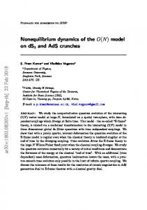
least one point inside typically decreases (shrinking of the Lebesgue measure) as 1/[1 + (qrel − 1) t/τq ]1/(qrel −1) (rel stands for relaxation; qrel ≥ 1; τq > 0 is a characteristic relaxation time). When applied to the chaos region (e.g., z = 2, a = 2), all these methods yield qsen = qrel = 1, in accordance with the usual BG concepts, founded on strongly chaotic systems, consistently with Boltzmann’s “molecular chaos” hypothesis (see [18] and references therein). When applied to the edge of chaos ac (z) of the z-logistic maps, it is obtained [17] qrel (∞) [qrel (∞) = 2.4... for z = 2]. In this Letter, we start with N points (we adopt N = 10 W for numerical convenience) uniformly distributed inside a single specific cell chosen as soon specified. We compute Sqsen (t) and verify that, for a fixed value of W , Sqsen (t) asymptotically reaches Sqsen (∞) [Sqsen (∞) > 0 monotonically increases with W ]. Sqsen (t) reaches its t → ∞ value from above, preceded by an overshooting, which might be very strong. The initial cell is chosen as that one which presents the highest overshooting. If we consider the strongly chaotic case a = 2, hence qsen = 1, S1 (t) slightly overshoots and rapidly saturates, as illustrated in Fig. 1(a) for z = 2. At the onset of chaos, however, Sqsen (t) presents a very pronounced overshoot, and slowly approaches its final value Sqsen (∞) [Fig. 1(b)]. We then compute, for all times after the overshooting, ∆Sqsen (t) ≡ [Sqsen (t) − Sqsen (∞)]. We find a power-law decay, whose log-log slope depends on W . (Log-periodic oscillations such as those reported in [17] are also detected here, and are better visualized for z < 2.). We identify this slope with 1/(qrel (W ) − 1) (as an alternative way of obtaining qrel ). In the limit W → ∞, we observe that qrel (∞) precisely coincides, for all values of z, with the value found in Ref. [17] (their values correspond to infinitely fine graining W → ∞). The powerlaw region of ∆Sqsen (t) increases with W (see Fig. 2). In order to better identify this region, we consider only those time intervals whose linear correlation coefficient is larger than 0.99. In order to increase the precision of qrel (W ) we take averages over various possible intervals, more precisely, ranging from various initial and various final times, as shown in Fig. 2. Moreover, in order to further minimize the effect [on the precision of qrel (W )] of the oscillations of Sqsen (t) at the onset of chaos, and also to better identify the attractor — the invariant distribution — we introduce a numerical improvement in the iteration rule which does not affect the asymptotic dynamics of the map: we average the distribution corresponding to xt with that corresponding to xt−1 (the actual values of x must be preserved while averaging). This procedure strongly reduces the considerable fluctuations in the distribution of points at t → ∞ and enables us to identify the attractor associated with the map (we refer to the attractor in the space of distributions, and not in phase space). The computer implementation of these numeri-

for which z = 2 recovers the logistic map, and partition the phase space into W cells of equal measure, pi being the probability to be soon associated with the ith cell. Several works [11–15] have shown that the description of such dynamical systems is properly achieved by using the nonextensive entropy, Eq. (1), with a specific z-dependent value of q. Let us first recall the sensitivity-based approaches, which determine qsen ≤ 1 (sen stands for sensitivity). Up to now, three different methods have been developed which provide the special value qsen (sometimes noted as q ∗ ). The first method [11] is based on the sensitivity to initial conditions. At the threshold of chaos [a = ac (z)], the Lyapunov exponent λ1 vanishes and the system is weakly sensitive (weak chaos), i.e., the upper bound separation between nearby trajectories ∆x(t) typically evolves [16] in time acξ(t) ≡ lim∆x(0)→0 ∆x(0) cording to the power-law 1

ξ(t) = [1 + (1 − qsen )λqsen t] 1−qsen

(λqsen > 0),

(2)

which is solution of the nonlinear differential equation ξ˙ = λqsen ξ qsen (this equation recovers, for qsen = 1, the usual exponential sensitivity to the initial conditions, referred to as strong chaos). The second method is based on the geometrical description of the multifractal attractor [12,13]. The value of qsen is determined by 1 1 1 1−qsen = αmin − αmax , where αmin and αmax are the values of the end points of the multifractal function f (α). This beautiful equation relates dynamics (left-hand side) with geometry (right-hand side). The third method is related, as we shall specify, to a conjectured generalization of the Pesin relation [14,15]. In one of the W cells in which the phase space has been divided, we initially put (randomly or uniformly distributed) N points (N ≫ W ). We then follow the occupancies {Ni (t)} of all PW cells [ i=1 Ni (t) = N ], which enable the calculation of the probabilities pi (t) ≡ Ni (t)/N , which enable in turn the calculation of Sq (t) as given by Eq. (1). We can next define a nonextensive version of the Kolmogorov-Sinai entropy, namely Kq ≡ limt→∞ limW →∞ limN →∞ Sq (t)/t. The special value q = qsen is the one for which the entropy production Kq is finite (if q < qsen , Kq → ∞, and if q > qsen , Kq → 0). It is quite remarkable that all three methods give (within an acceptable numerical error) one and the same value for qsen (qsen = 0.2445... for z = 2). Let us now turn to the relaxation-based approach of the problem, first tackled in [17]. We start now [17] with an ensemble of initial conditions uniformly spread over the entire phase space (a procedure that resembles the Gibbsian approach of statistical mechanics), instead of within a single among the W cells (closer to a Boltzmannian approach), and investigate the rate of convergence onto the multifractal attractor at the onset of chaos. At 1−q t = 0 all W cells are occupied (hence Sq = W 1−q−1 ). As t increases, the number Woccupied of cells that have at 2

cal benefits demands additional memory and an increase of the CPU time. The oscillations that remain are considerably smaller, and they can be further reduced by extending the method in order to take into account more than one previous time step. However, for the accuracy we seek in this work, it is clearly enough to average the distributions of xt−1 and xt . We emphasize that this kind of averaging is just a trick to minimize the fluctuations (the original dynamics is preserved, once we average the distribution of x, and not x itself). If the procedure is not adopted, we find the same results, though with less precision. After all these numerical improvements have been implemented, a remarkable law emerges, namely, qrel (∞) − qrel (W ) ∝ W −|qsen |

dynamics is dictated by noninteracting or short-range interacting particles is described by Boltzmann-Gibbs statistical mechanics, and usual thermodynamics apply, typically together with the usual exponential relaxation to equilibrium. But for systems with complex dynamics (complex in the sense previously described), we cannot know a priori how the relaxation to the stationary state occurs. However, for a vast class of such systems, powerlaw relaxation does occur. To determine the associated exponent we must analyze at least once the dynamics of that particular nonextensivity universality class, in such a way as to determine once the corresponding values of q. For z-logistic maps, Eq. (3) (main result of the present work) gives the connection between those values of q. The analogous task for Hamiltonian systems would be very welcome.

(3)

(see Fig. 3). This equation is somehow analogous to the expressions that appear in finite-size scaling [19]. This law is quite impressive, since it relates two basic dynamical properties of dissipative systems, namely, relaxation onto equilibrium and sensitivity to the initial conditions (the basis for mixing). Moreover, the (coarser or finer) graining — 1/W for the z-logistic maps — is involved, pretty much in the same way as it occurs with the values of q (here noted as qrel ) appearing in Beck’s approach [3] of fully developed turbulence, where the entropic index depends on the distance between the two points at which the fluid velocities are measured. Other phenomena where a similar scaling relation may occur are the distribution of transverse momenta of hadronic jets produced in electron-positron annihilation experiments [5], and the saddle-point dynamics of the Henon-Heiles system [20]. Let us also mention that the scaling relation, Eq. (3), has a moderate sensitivity to the value used for qsen (see the Inset of Fig. 3). It is important to emphasize that Eq. (3) reflects the fact that the limits limt→∞ limW →∞ (relevant for qsen ; see for instance [14]) and limW →∞ limt→∞ (relevant for qrel , as exhibited here) do not commute (nonuniform convergence) in general (in other words, generically qsen 6= qrel , whereas for strong chaos it is qsen = qrel = 1). This result is similar to the noncommuting t → ∞ and M → ∞ limits for long-range interacting M -body Hamiltonian systems [21], for which vanishing Lyapunov exponents have already been detected [22] (we remind that these limits do commute for short-range interactions). We finally exhibit Fig. 4, which shows qrel (∞), as well as qsen (taken from [11]), for typical values of z. For qrel (∞) we have indeed verified the coincidence (with high precision for all z) with the values observed in [17] by starting with uniform occupation of the phase space and following the shrinking of the Lebesgue measure. In addition to these results, we observe that qsen (z → ∞) ≃ 0.72 and limW →∞ qrel (z → 1) ≃ 4/3. In conclusion, the scenario which emerges is that the thermal equilibrium of all Hamiltonian systems whose

ACKNOWLEDGMENTS

One of us (CT) thanks H.J. Herrmann for fruitful remarks. This work is partially supported by PRONEX/MCT, CNPq, CAPES and FAPERJ (Brazilian agencies).

[1] E.G.D. Cohen, Physica A 305, 19 (2002). [2] M. Baranger, Physica A 305, 27 (2002). [3] C. Beck, G. S. Lewis and H. L. Swinney, Phys. Rev. E 63, 035303 (2001); C. Beck, Phys. Rev. Lett. 87, 180601 (2001) and references therein. [4] T. Arimitsu and N. Arimitsu, Physica A 305, 218 (2002) and references therein. [5] I. Bediaga, E. M. F. Curado and J. Miranda, Physica A 286, 156 (2000). [6] L. Borland, Phys. Rev. Lett. 89, 098701 (2002). [7] A. Upadhyaya, J.-P. Rieu, J.A. Glazier and Y. Sawada, Physica A 293, 549 (2001). [8] C. Tsallis, J. Stat. Phys. 52, 479-487 (1988). [9] E. M. F. Curado and C. Tsallis, J. Phys. A: Math. Gen. 24, L69-72 (1991); Corrigenda: 24, 3187 (1991) and 25, 1019 (1992); C. Tsallis, R. S. Mendes and A. R. Plastino, Physica A 261, 534 (1998). [10] C. Tsallis, in Nonextensive Statistical Mechanics and Its Applications, edited by S. Abe and Y. Okamoto, Lecture Notes in Physics Vol. 560 (Springer-Verlag, Berlin, 2001), p.3; C. Tsallis, E. P. Borges, and F. Baldovin, Physica A 305, 1 (2002); Non Extensive Statistical Mechanics and Physical Applications, edited by G. Kaniadakis, M. Lissia, and A. Rapisarda (Elsevier, Amsterdam, 2002); Nonextensive Entropy – Interdisciplinary Applications, edited by M. Gell-Mann and C. Tsallis (Oxford University, New York, to be published). An

3

[11] [12] [13] [14] [15] [16]

[17] F. A. B. F. de Moura, U. Tirnakli, M. L. Lyra, Phys. Rev. E 62, 6361 (2000). [18] J. A. S. de Lima, R. Silva and A. R. Plastino, Phys. Rev. Lett. 86, 2938 (2001). [19] M. N. Barber, Finite-size Scaling, in Phase Transitions and Critical Phenomena, Vol. 8, eds. C. Domb and J. L. Lebowitz (Academic Press, London, 1983). [20] H. P. de Oliveira, I. D. Soares and E. V. Tonini, Physica A 295, 348 (2001). [21] V. Latora, A. Rapisarda and C. Tsallis, Phys. Rev. E 64, 056134 (2001). [22] C. Anteneodo and C. Tsallis, Phys. Rev. Lett 80, 5313 (1998).

updated bibliography can be found at the web page http://tsallis.cat.cbpf.br/biblio.htm U. M. S. Costa, M. L. Lyra, A. R. Plastino and C. Tsallis, Phys. Rev. E 56, 245 (1997) and references therein. M. L. Lyra and C. Tsallis, Phys. Rev. Lett. 80, 53 (1998) and references therein. U. Tirnakli, C. Tsallis and M. L. Lyra, Eur. Phys. J. B 11, 309 (1999). V. Latora, M. Baranger, A. Rapisarda, C. Tsallis, Phys. Lett. A 273, 97 (2000). U. Tirnakli, G. F. J. Ananos, C. Tsallis, Phys. Lett. A 289, 51 (2001). F. Baldovin and A. Robledo, Phys. Rev. E 66, 045104 (2002); Europhys. Lett. 60, 518 (2002).

4

15 10

(a)

z=2 a=2 W = 512 000 W = 256 000 W = 128 000 W = 64 000

S1 5 0 0

5

10

15

20

25

30

t 25000 20000 S0.2445

z = 2 a = 1.401155189... (b) W = 512 000

W = 256 000

15000

W = 128 000

10000

W = 64 000

5000 0

0

50

100 150 200 250 300

t FIG. 1. Sqsen (t) for z = 2 . (a) Chaotic region, with qsen = 1; (b) Edge of chaos, with qsen = 0.2445, associated to the region before the peak [12,14], and with qrel (W ) > 1, associated to the region after the peak. (the highest value attained by S0.2445 , for a given W , is about 70% of the value corresponding to equiprobability). Notice that for a = 2, the stationary state is achieved for t much smaller than that for a = ac , which of course reflects the fact that relaxation is exponentially quick in the former (as it is also the case for a < ac ) whereas it is a power-law in the latter.

5

5

10

W = 64 000 W = 128 000 W = 256 000 W = 512 000

4

∆S0.2445(t)

10

3

10

2

10

z=2 1

10

a = 1.401155189...

0

10 10

100

t

1000

10000

FIG. 2. ∆Sqsen (t) ≡ Sqsen (t) − Sqsen (∞) at the z = 2 chaos threshold, for typical W . For each W we consider as the power-law region (linear correlation coefficient above 0.99) that going from the left interval to the right one. Furthermore, the values for qrel (W ) in Fig. 3 were obtained by averaging over many starting (ending) points inside the left (right) interval.

6

4.0 1.000

z=2 0.999

z = 5.0

3.0

R

0.998

0.997 0.15 z = 3.0

q rel

0.2

0.25

0.3

q sen

z = 2.0 2.0

z = 1.5 1.0

0

0.2

0.4

( W/1000 )

_|q

sen

0.6

0.8

|

FIG. 3. W -dependence of qrel for typical values of z. The W → ∞ extrapolated values coincide with the values reported in [17]. The abscissa has been chosen to be (W/1000)−|qsen | (instead of W −|qsen | ) for better visualization. Inset: Linear correlation coefficient procedure which has been used to select a specific numerical value for the sensitivity entropic index qsen (z).

7

4

q rel (∞) 2 4/3 0.72

q sen

0

q

3

q

q

2 1 0

1

0.58

2

3

(z-1) -6

1

-2 -4

4/3

-4

(b)

0

rel

-2

0.72

(a)

sen

(z)

4

0

0.5

1.7

1

1/z

2

3

z

4

5

FIG. 4. z-dependences of qsen (from [11], or self-consistently through Eq. (3)) and qrel (∞). Inset (a): z → 1 extrapolation for qrel (∞); qrel (∞) = 4/3 + 1.077(z − 1)0.58 fits the z ≤ 3.0 data. Inset (b): z → ∞ extrapolation for qsen (∞); qsen (z) = 0.72 − 1.525/z 1.7 fits the z ≥ 1.75 data.

8