Visualizing the logistic map with a microcontroller
arXiv:1112.5791v1 [nlin.CD] 25 Dec 2011
Juan D. Serna∗ School of Mathematical and Natural Sciences University of Arkansas at Monticello, Monticello, AR 71656 Amitabh Joshi† Department of Physics Eastern Illinois University, Charleston, IL 61920 December 25, 2011
Abstract The logistic map is one of the simplest nonlinear dynamical systems that clearly exhibit the route to chaos. In this paper, we explored the evolution of the logistic map using an open-source microcontroller connected to an array of light emitting diodes (LEDs). We divided the onedimensional interval [0, 1] into ten equal parts, and associated and LED to each segment. Every time an iteration took place a corresponding LED turned on indicating the value returned by the logistic map. By changing some initial conditions of the system, we observed the transition from order to chaos exhibited by the map.
1
Introduction
Nonlinear dynamics is a topic that not only cover all the disciplines, in both natural and social sciences, but also is now becoming part of introductory level undergraduate courses in sciences. Searching for affordable, easy to setup, and reconfigurable classroom demonstrations that allow to investigate the physical and mathematical nature of nonlinear dynamical systems has been always a matter of interest for instructors. This paper describes a simple apparatus used to explore the behavior of one-dimensional chaotic maps, like the Logistic Map, when different initial conditions are chosen. The device consists of an inexpensive open-source microcontroller connected to an array of light emitting diodes (LEDs), and programmed to iterate the logistic map in the one-dimensional interval [0, 1]. This interval is divided in ten equal parts and mapped one-to-one to a single LED in the array. When the logistic map produces certain value after an iteration, the corresponding LED lights up showing the value in the one dimensional domain approximately. After several iterations, it is possible to visualize the trajectory of the map by looking at the blinking LEDs sequence. Sensitivity to initial conditions, density of periodic orbits, strange attractors, and bifurcations are visualized easily with this device. ∗ †
[email protected] [email protected]
1
2
One dimensional maps
The logistic map is, perhaps, the simplest example of how a nonlinear dynamical equation can give rise to very complex, chaotic behavior. 1 Initially introduced as a mathematical model of population growth, 2 it rapidly found applications in diverse areas like mathematical biology, biometry, demography, condense matter, econophysics, and computation. 3 The logistic map function is defined as Xn+1 = A Xn (1 − Xn ) ≡ fA (X), (1) where the factor A is a model-dependent parameter representing external conditions to the system, and Xn is the population in the nth-period cycle, scaled so that its value fits in the interval [0, 1]. 4 The function fA is called an iteration function because we may find the population fraction X in the following period cycle by repeating the mathematical operations expressed in (1). 5 It is also one-dimensional since there is only a single variable X, and the resulting curve is a line.
3
Setup
We show a photograph of the apparatus setup in Fig. 1, and its schematics in Fig. 2.
Figure 1: Setup of the Logistic Map device. An array of ten LEDs are connected to the Arduino microcontroller using the same number of 220 Ω resistors. The apparatus uses an open-source Arduino prototyping platform made up of an Atmel AVR processor (microcontroller). It has 14 digital input/output pins, 6 analog inputs, a 16 MHz crystal oscillator, a USB connection, a power jack, an ICSP header, and a reset button. 6 Arduino is a registered trademark—only the official boards are named “Arduino”—so clones usually have names ending with “duino.” 7 The Arduino can be connected to a computer through the USB port and programmed using a language similar to C++. The program is uploaded into the microcontroller using an Integrated Development Environment (IDE). In the Arduino world, programs are known as sketches. We connected an array of ten 5 mm LEDs to the digital pins of the microcontroller using 220 Ω resistors (or 1 kΩ for dimmer LEDs). We also used a solderless breadboard to hook up all the electric components to the microcontroller. 2
Figure 2: Circuit diagram of the ten LEDs array connected to the Arduino.
4
The sketch
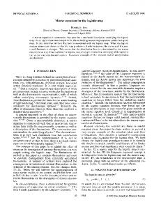
Listing 1 shows a simple program (sketch) used to operate the microcontroller, and visualize the logistic map by looking at the array of blinking LEDs. A glowing LED represents an iteration of the one-dimensional map, and it is linked with a value in the interval [0, 1]. Arduino programs require two mandatory functions: setup() and loop(). Any variable or constant defined outside these two functions is considered to be global. In the setup() function, we tell the microcontroller that there are 10 LEDs connected to the digital pins and that they are intended to be turned on and off. In the loop() function, the logistic map is iterated, and the visualization process takes place as we observe the LEDs turning on and off, one after another, following the evolution of the nonlinear system. Using the if() and else control structures, we divide the interval [0, 1] in ten identical segments and associate an LED to each one of them. For example, the first LED from the left represents the first interval segment [0, 0.1), the second LED represents the segment [0.1, 0.2), and so on. The last LED represents the final segment [0.9, 1.0]. When the microcontroller iterates the logistic map, a value belonging to one of these ten intervals is returned, and the corresponding LED turns on for 500 milliseconds. This process is repeated infinitely, so we can observe the orbit followed by the logistic map by watching at the blinking LEDs sequence. The initial conditions for the logistic map can be changed anytime and uploaded again into the microcontroller. Thus, we can explore the behavior of the chaotic map when different values of the parameters A and X0 are chosen. It is amusing to study the bifurcations of the logistic map by looking at the blinking sequence of LEDs. We start with the parameter values A = 0.9 and X0 = 0.5 (0 < A < 1). The LED associated with the interval [0.5, 0.6) turns on first. As the iterations of the logistic map take place, we observe that the sequence of blinking LEDs moves toward the very first LED, which is associated with the segment [0, 0.1). The sequence ends up with this first LED left on indefinitely. This evolution is shown in Fig. 3(a), the cobweb diagram of the logistic map for that selection of parameters. For this case, X = 0 is an attractor, and the domain [0, 1] forms a basin of attraction. Another example of an attractor happens when A = 2.9 and X0 = 0.2 (1 < A < 3). We see 3
Figure 3: Cobweb diagrams for the logistic map for different values of A and X0 . The 45◦ line, Xn+1 = Xn , is used to find the fixed points and follow the iteration process. Plots (a) and (b) show the presence of attractors at X = 0 and X = 0.655, respectively. Plot (c) displays a period doubling bifurcation, and (d) the onset of chaos. that, after few iterations and blinking LEDs, there is only one LED that remains on indefinitely. This LED corresponds to the interval [0.6, 0.7). In this case, we have a fixed point occurring at X = 0.655. As it is shown in Fig. 3(b), the orbit of the map follows a square spiral that converges into that fixed point. Now, if A = 3.1 and X0 = 0.2 (3 < A < 3.44948), we can observe a 2-period cycle; the value of X oscillates between 0.558 and 0.765, and the two corresponding LEDs turn on and off intermittently. Here, the fixed point X = 0.677 becomes a repeller. Figure 3(c) shows the periodic behavior of the logistic map for this set of parameters. Unfortunately, higher periodicity (like 4-period, 8-period cycles, or higher) cannot be observed clearly with this device because of the way the LEDs are mapped into the [0, 1] interval. More LEDs are required to improve the “resolution” of the device. However, the microcontroller has a limit of 13 digital pins, and other electric components (like an extra microchip) need to be incorporated into the circuit if we want more LEDs controlled by the device. Finally, when A = 3.7 and X0 = 0.05 (3.56994 < A < 4), chaos onsets. 8 An “apparently” randomness of blinking LEDs is observed. After many iterations, there is no single LED that remains on indefinitely, and no single LED that has not been turned on at least once. The orbit of the logistic map covers all the domain of the interval [0, 1]. Figure 3(d) shows all points visited by the logistic map orbit after 10 000 iterations.
4
5
Final comments
With this apparatus, students may understand more easily the behavior of one-dimensional chaotic maps looking at an actual one-dimensional array of LEDs; every point in the interval [0,1] produces another point within the same interval after the logistic map is iterated. By controlling the parameter A and the initial value X0 , the instructor and students can observe under what conditions periodic and chaotic behavior may occur, providing a better understanding of periodicity, bifurcations, and the route to chaos of a nonlinear dynamical system. The setup described here is inexpensive, easy, and fun to assemble, also enhances computer programming and electronics assembly skills.
References 1. E. W. Weisstein, “Logistic Map.” From MathWorld–A Wolfram Web Resource. http://mathworld.wolfram.com/LogisticMap.html 2. P.-F. Verhulst, “Recherches math´ematiques sur la doi d’accroissement de la population,” Mem. Acad. Royale Belg. 20, 1–32 (1847). 3. M. Ausloos and M. Dirickx (eds.), The Logistic Map and the Route to Chaos : From the Beginnings to Modern Applications, (Springer, New York, 2006). 4. J. B. Marion and S. T. Thornton, Classical Dynamics of Particles and Systems, 4th ed. (Saunders, Fort Worth, 1995), p. 178. 5. R. C. Hilborn, Chaos and Nonlinear Dynamics, 2nd ed. (Oxford, New York, 1994), p. 19. 6. Arduino: www.arduino.cc 7. M. Schmidt, Arduino: A Quick-Start Guide, (Pragmatic Bookshelf, Raleigh, 2011). 8. J. C. Sprott, Chaos and Time-Series Analysis (Oxford, New York, 2003).
5
// B l i n k i n g L o g i s t i c Map // c h o o s e th e p i n f o r each LED const i n t NbrLEDs = 1 0 ; const i n t LEDpin [ ] = { 2 , 3 , 4 , 5 , 6 , 7 , 8 , 9 , 1 0 , 1 1 } ; const i n t w a i t = 5 0 0 ;
// w a i t f o r 500 m i l l i s e c o n d s
// L o g i s t i c Map p a r a m e te r s const double A = 3 . 7 ; // L o g i s t i c map c o n s t a n t double X0 = 0 . 2 ; double X = X0 ;
// I n i t i a l p o s i t i o n (0 < X0 < 1 . 0 ) // Use X0 a s your f i r s t c a l c u l a t e d p o i n t
// s e t u p ( ) i n i t i a l i z e s th e LED p i n s void s e t u p ( ) { f o r ( i n t i = 0 ; i < NbrLEDs ; i ++) { pinMode( LEDpin [ i ] , OUTPUT) ; } } // l o o p ( ) i t e r a t e s th e L o g i s t i c void l o o p ( ) { i f (X < 0 . 1 ) blinkLED ( LEDpin [ 0 ] ) ; e l s e i f ( (X >= 0 . 1 ) && (X < blinkLED ( LEDpin [ 1 ] ) ; e l s e i f ( (X >= 0 . 2 ) && (X < blinkLED ( LEDpin [ 2 ] ) ; e l s e i f ( (X >= 0 . 3 ) && (X < blinkLED ( LEDpin [ 3 ] ) ; e l s e i f ( (X >= 0 . 4 ) && (X < blinkLED ( LEDpin [ 4 ] ) ; e l s e i f ( (X >= 0 . 5 ) && (X < blinkLED ( LEDpin [ 5 ] ) ; e l s e i f ( (X >= 0 . 6 ) && (X < blinkLED ( LEDpin [ 6 ] ) ; e l s e i f ( (X >= 0 . 7 ) && (X < blinkLED ( LEDpin [ 7 ] ) ; e l s e i f ( (X >= 0 . 8 ) && (X < blinkLED ( LEDpin [ 8 ] ) ; else blinkLED ( LEDpin [ 9 ] ) ;
Map and tu r n on / o f f LEDs
0.2)) 0.3)) 0.4)) 0.5)) 0.6)) 0.7)) 0.8)) 0.9))
// i t e r a t e s th e L o g i s t i c Map f u n c t i o n X0 = X; X = A ∗ X0 ∗ ( 1 . 0 − X0 ) ; } // blinkLED f u n c t i o n // tu r n on / o f f LEDs void blinkLED ( const i n t p i n ) { digitalWrite ( pin , HIGH ) ; // tu r n LED on delay ( w a i t ) ; // w a i t 500 m i l l i s e c o n d s digitalWrite ( pin , LOW) ; // tu r n LED o f f }
Listing 1: Logistic Map sketch for the Arduino.
6