Nonlinear Decoupling Control for a Class of Continuous ... - wseas.us

Nonlinear Decoupling Control for a Class of Continuous Stirred Tank Reactors A.S.TSIRIKOS1,2 and N.E.MASTORAKIS2 (1)NATIONAL TECHNICAL UNIVERSITY OF ATHENS DIVISION OF COMPUTER SCIENCE DEPARTMENT OF ELECTRICAL AND COMPUTER ENGINEERING 15773 ZOGRAPHOU, ATHENS, GREECE (2)MILITARY INSTITUTIONS OF UNIVERSITY EDUCATION HELLENIC NAVAL ACADEMY CHAIR OF COMPUTER SCIENCE 18539, HATZIKYRIAKOY, PIRAEUS, GREECE

Abstract. In this paper a new approach to the decoupling control problem using static state feedback is applied to the nonlinear model of a class of continuous stirred tank reactors(CSTR). The main feature of this approach is that it reduces the problem of determining the admissible state feedback control law to the solution of a system of first order partial differential equations. Based on these equations, necessary and sufficient conditions for the problem to have a solution as well as the general analytical solution for the admissible feedback control laws are derived. Applying this approach to a CSTR , the general analytical expression for the control law is produced. Moreover, it is proven that appropriate choise of the three parameters of the control law leads to a closed-loop system with linear input-output (i/o) description and arbitrarily assigned eigenvalues.

1. Introduction Rapid changes in market demands and economics move operation of chemical reactors towards operating points where nonlinearity and interaction are dominant features. As a result, regulatory as well as servo control of chemical reactors can be extremely difficult [1]. Conventional linear controllers may perform poorly when used to control nonlinear processes because it is difficult to combine good performance with acceptable stability margins [2]. Thus, most of the industrial chemical reactors are controlled with simple nonlinear control elements [1],[2]. However, due to limited heat removal, improper tuning of such controllers can increase the risk of thermal runaways. For such nonlinear processes, controller design strategies based directly on nonlinear models can provide improved performance. This has been proven to hold true for a number of chemical processes [3],[4]. Recently, a general nonlinear control theory based on differential geometry has emerged,[5]. An extensive survey of process control applications is presented in [6]. The decoupling problem of nonlinear systems has received much attention in the past [5],[7]-[12]. In [5] and [7] the first systematic results are reported. In [5], a geometric

approach to the decoupling control problem is presented, in particular, necessary and sufficient criteria, of geometric nature, for the problem to have a solution are established. A characterisation of all decoupling control laws has been reported in [8], wherein the determination of the decoupling control law requires the solution of a homogeneous system of first order partial differential equations (whose solution, in general, is not constructable). In [9], a construction algorithm of the decoupling control laws has been presented. In this paper a new approach to the decoupling problem under static state feedback is presented. The proposed approach reduces the determination of the desired control law to the determination of the desired control law to the solution of a nonhomogeneous system of first order partial differential equations. On the basis of the decoupling design equations, the necessary and sufficient conditions [5], [7]-[9], for the problem to have a solution, are easily rederived. In addition, the general expression of the desired control law is derived and a constructive algorithm of all the admissible controllers is presented. This algorithm requires only simple integration. It is noted that application of the general solution of the control law may lead to stable internal dynamics, in case where special solutions of the control law result to unstable internal dynamics [8]. The foregoing decoupling technique, is applied to the nonlinear model of a class of CSTR. It is proven that for the particular class of CSTR, the decoupling problem is solvable. Moreover, the most general solution for the admissible control law is analytically derived. Application of the decoupling control law to the CSTR leads to a closed-loop system with linear i/o description and arbitrarily assigned eigenvalues. The results presented in this paper form part of the material reported in [10]. Detailed results on the decoupling problem on nonlinear systems via state feedback are presented in [11]. The present method has been extended to cover the more general case of simultaneous decoupling and disturbance rejection of nonlinear systems are reported in [12].

2. The Decoupling Technique [10], [11] 2.1. Preliminaries Consider the nonlinear analytic system •

x = g 0 (x ) + G (x )u , x(0 ) = x 0 ,

y = h(x )

(2.1)

where u,y ∈Rm and the state x belongs to an open subset U of Rn . The vector g 0 (x ) , each column g i (x ) of G (x ) and h(x ) are analytic vector valued functions of x from U to Rn and Rm , respectively. Definition 2.1. The characteristic numbers di 's, ∀i∈{1,.....,m}, are defined as L g j Lkg 0 hi (x ) = 0 , ∀ j∈{1,2,...,m} and k < di Lg j Lg 0

di

hi (x ) ≠ 0, for some j∈{1,2,....,m}

∀x around x0 , where Lτ (.) denotes the Lie derivative with respect to τ , [13], and hi ( x ) is the i-th component of h(x).

2.2. The Decoupling Technique Definition 2.2. A system of the form (2.1) is i/o decoupled, if the i-th element of the input u affects only the i-th element of the output y for any x around xo Statement of the Decoupling problem: Consider applying to system (2.1) the control law u = a(x) + B(x)w (2.2) m where w∈ R and B(x) is nonsingular, for any x around x0 , to yield the closed loop system •

−

−

x = g 0 (x ) + G (x )u , x(0 ) = x 0 ,

y cls = h( x )

(2.3a)

g 0 (x ) = g 0 (x ) + G (x )a(x ) , G (x ) = G ( x )B (x )

(2.3b)

where −

−

The decoupling problem is defined as follows [10]: Determine a control law of the form (2.2) such that the resulting closed loop system (2.3) is i/o decoupled. We will present here the main theorems established in [10] and [11]. Decoupling Design Equations Theorem 2.1. Assume that B(x ) ≠ 0, ∀x around x0 . Then, the unknown pair {a(x), B(x)} satisfies the following set of equations, called the (DDE) B ∗ (x )B (x ) = diag { λ i (x ) }

Decoupling Design Equations

(2.4)

i∈{1,..., m }

ϑi (x )Π i (x ) =0 ξ i (x )Π i (x ) =0 where

ϑi (x ) = [dϕ i (x )M k i (x )M k i , 0 (x )ML]

ξ i (x ) = [dλ i (x )M pi (x )M pi , 0 (x )ML]   d  Π i (x ) =  d  d  

(2.5) (2.6)

[G[g 1 , G ]K[g m , G ][g 0 , G ]K] (Ldg hi )[G[g 1 , G ]K[g m , G ][g 0 , G ]K] (Ldg hi )[0 0 K 0 G K]   (Ldg hi )[0 0 K 0 0 K]  i

0

i

0

i

0

M

M

M

M

 

(2.7)

where d(.) denotes the usual gradient, τ , σ denotes the Lie bracket operation [13], ∆

φ i (x ) = L −i hi , λ i (x ) ≠ 0, Κ i (x ) , Κ i , 0 (x ) ,....... and pi (x ) , p i , 0 (x ) ,... depend on the d +1 g0

Markov parameters of the closed loop system, and  d d1 h1 (x )  L g0  ∆  ∗ G B (x ) =  M   dm  d L g 0 hm (x ) 

(

)

(

)

Necessary and Sufficient Conditions: Based on the DDE, the necessary and sufficient conditions for the decoupling problem to have a solution may be established. These conditions are given by the following Theorem [10], [11] (see also [5], [7]-[9]). Theorem 2.2. The necessary and sufficient conditions for the solvability of the decoupling problem are det B ∗ (x ) ≠ 0, ∀x around x0

[

]

Special Solution for the Control Law:

∧

∧

If Theorem 2.2 is satisfied, then a special solution {a (x), B (x)} for the control law (2.2) , which satisfies the decoupling problem is

[

∧

]

a (x)=- B ∗ (x ) where

∆

a ∗ (x ) =

[L

d1 +1 g0

−1

h1 (x ) K L gm0 hm (x ) d +1

]

Τ

[

∧

a ∗ (x )

]

B (x)= B ∗ (x )

and

−1

(2.8)

. The special solution (2.8) is often called in the

literature as the "standard noninteracting feedback" [5] and [13]. Application of the special pair (2.8) to (2.1) results in the closed-loop system •

∧

∧

x = g 0 (x ) + G (x )u , x(0)=x0 ∧

∆

∧

and ∧

∆

y=h(x)

(2.9)

∧

where g 0 (x ) = g 0 (x ) + G (x ) a(x ) and G (x ) = G(x)B (x).It is easy to see that the closed-loop system (2.9) may be separated into m subsystems having i/o maps of the form

y

( d i +1) i

=wi

General Solution for the Control Law: Based on the DDE, the general expression for the control law (2.2) is given by the following theorem [10] and [11]. Theorem 2.3. If Theorem 2.2 is satisfied , then the general solution for the pair {a(x), B(x)} of the control law (2.2) will be given by

[

]

a(x)=- B ∗ (x ) { a ∗ (x ) - φ (x ) } −1

(2.10a)

[

]

B(x)= B ∗ (x ) ∆

−1

diag { λ i (x ) }

(2.10b)

i∈J m

where φ (x ) = [φ1 (x ), K, φ m (x )] . The functions φ i (x ) and λ i (x ) are defined as follows Τ

∧

∧

∧

∧

∧

∧

∧

∧

φi =φi ( t i ,1 (x ), K , t i ,σ i (x ), s i ,1 (x ), K, s i ,n − n (x ) ) *

(2.11)

λ i =λ i ( t i ,1 (x ), K , t i ,σ i (x ), s i ,1 (x ), K, s i ,n − n (x ) ) (2.12) where φi and λ i ≠ 0 are arbitrary analytic functions of their arguments with λ i ≠ 0. ∧

*

∧

To determine t i , ρ (x ) , ρ ∈ {1,........,σi } and s i , ρ (x ) , ρ ∈ {1,........,n − n∗ }, for i∈{1,2,....m}, as well as the integers n∗ and σi , the following algorithm has been proposed ([10], [11]). Construction algorithm for φi , λ i , i∈{1,2,......m} ∧

Step 1 Construct the reachability matrix Q(x ) of the closed loop system (2.9) ∧ ∧   ∧    Q(x ) = G MKM g j1 , K , g jk , G  K           where j1 ,......, jk ∈{0,1,....,m} and k∈{0,1,2,...}. The integer n∗ is defined by ∧  n∗ =rank Q(x ) , ∀x around x0 (2.14)   ∧

∧

Step 2 Construct the matrix S i (x )  ∧  ∧ ∧   X ki = g j1 , K , g jk , g i       ∧

∧

where j1,......, j k ∈ {0,i}, k∈{0,1,2,...}. The rest of the columns of Q(x ) form the ∧

matrix S ci (x ) . The number ni is defined as the dimension of the involutive closure, [13] , of the distribution spanned, locally around x0 , by the columns of the matrix ∧

S ci (x ) , i.e. ∧

ni =dim{inv[ S ci (x ) ]}, ∀x around x0

(2.15)

Step 3 Define the following integers σi = n∗ − ni ∧

Step 4 Rearrange the columns of the reachability matrix Q(x ) as follows ∧ ∧ ∧  Q(x ) = L ic (x )M L i (x )  

(2.16)

where ∧

∆

∧

∧

di ∧

L ic (x ) = [inv[ S ci (x ) ] M g i (x )MKM adg∧0 g i (x )

(2.17)

Step 5 Find a local base of the distribution spanned by the columns of the matrix ∧

L ic (x ) . Denote it as follows ∧ I 

c i ,1



∧

(x )MKM I ci,n + d +1 (x ) i



i

∧

Step 6 Construct the matrix R i (x ) , the columns of which constitute a local base of ∧

the distribution spanned by the columns of Q(x ) , as ∧ ∧ R i (x ) =  I 

c i ,1



∧

(x )MKM I i,n +σ (x ) i



i

(2.18)

where ∧

I

∧

i , ni + d i + 2

(x ),K , I i,n +σ (x ) i

i

∧

are the Linear independent columns of L i (x ) which are also Linearly independent ∧

from the columns of L ic (x ) . Step 7 Construct the matrix ∧

R ∧

# i

∧

∧

∧

(x ) =[ R i (x )M d i,1 (x )MKMd i,n −n (x ) ] ∗

(2.19)

∧

∧

where d i ,1 (x )MKMd i , n −n∗ (x ) are nx1 vectors orthogonal to the matrix R i (x ) , such that the d Τi, j (x ) are complete differentials. ∧

∧

Step 8 The functions t i , ρ (x ) and s i , ρ (x ) are the solutions of the following first order partial differential equations ∧  ∧ d  t i , ρ (x ) = w i , ρ (x ) , ρ ∈ {1,...,σi } (2.20)   ∧  ∧ d  s i , ρ (x ) = d  

Τ i, ρ

(x ) ,

ρ ∈ {1,...,n − n∗ }

(2.21)

where ∧ ∆ ρ w i , ρ (x ) = (− 1) d  Ld∧i +1− ρ h i  , ρ ∈ {1,...,di +1}  g0  −1

∧#  w i , ρ (x ) = e ∗  R i (x ) , ρ ∈ {di +2,...,σi } n −σ i + ρ   ∧

and e ∗

n −σ i + ρ

∆

(2.21a)

Τ

(2.21b)

denotes the (n∗ − σi + ρ)-th column of In . It is noted that the first order

partial differential equations (2.20) may be solved by a simple integration. m

Remark 2.1. If

∑ (d i =1

by

i

+ 1) =n∗ =n, then the solution for the functions φi and λ i is given

φi =φi (hi ,...,Ldi∧ hi ) and λ i =λ i (hi ,...,Ldi∧ hi ) g0

(2.22)

g0

Remark 2.2 In [10] it is proven that there exist σi linearly independent solutions for φi or λ i of the DDE. Furthermore, it is proven that the functions hi (x ) ,..., Ld∧i h i (x ) are g0

linearly independent and they are also solutions for φi orλ i . Hence σi ≥ di +1. Remark 2.3 If σi =di +1, and n=n∗ then the general solution for φi and λ i . may be immediately determined by (2.22)

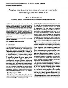
3. The chemical reactor mathematical model and control problem A typical chemical reactor is given in figure 1.

Figure.1 A typical chemical reactor

The reactants are feed to the reactor where we assume that the following successive reactions take place k1 k2 A  → B  →C where the reactant forms an intermediate product, the desired product (B), which reacts further to form another product, the undesired product (C). This general scheme is of considerable practical importance in a number of chemical processing operations [14], [15]. The heat released by the above exothermic reactions is removed by a coolant medium circulated through the jacket. The concentration CΑΟ of the species A in the feed and cooling rate Q are the manipulation variables. The outputs of the system are the temperature T in the reactor and the concentration CB of the desired

product. The control problem consists of maintaining the values of the controlled variables T and CB around specified values in spite of interactions and/or disturbances. By assuming constant properties, the CSTR may be described by the following equations: dC A V =F( C Α0 -CA )-V K 1 (Τ) CAn1 (3.1a) dt © dC B V =F(-CB )+V K 1 (Τ) CAn1 -V K 2 (Τ) CBn2 (3.1b) dt © dT V Q V =F(T0 -T)+ ((-∆Η1 ) K 1 (Τ) CAn1 +(-∆Η 2 ) K 2 (Τ) CBn2 )+ (3.1c) ρCp ρCp dt © The reaction rate constants K i (Τ) , i=1,2, follow the Arrhenius temperature dependency. The above model may be put in dimensionless form by defining new variables,as follows x1 =CA CAr , x2 =CB CA , x3 =T T0 u1 =CA0 CAr , u2 =Q, y1= x2 , y 2 = x3 n1 −1 n2 −1 1 F K10CAr V K20CAr V Da1= , t=t' , Da2 = , β= F F ρCρ FT0 V (− ∆Η1 )C Ar , = (− ∆Η 2 )C Ar ,δ = E1 , δ = E2 H1= H2 1 2 RT0 RT0 ρC p T0 ρC p T0 Hence the model of the CSTR can be written as •

∆

x =f(x) + G(x)u, y=h(x)

(3.2)

where f(x)= g 0 (x ) and

x= [x 1 x 2 x 3 ] , u = [u1 u 2 ] , y= x2 x3 , T

T

T

[ ( ) f (x ) f (x )]

f(x)= f 1 x

T

2

3

f1 (x ) =- x1 - Da1 x1n1 e − (δ1 x3 ) f 2 (x ) =- x 2 + Da1 x1n1 e − (δ 1 x3 ) − Da 2 x 2n2 e − (δ 2 f 3 (x ) =1- x3 + Da1 H 1 x1n1 e − (δ 1

x3 )

x3 )

+ Da 2 H 2 x 2n2 e − (δ 2

x3 )

1M 0  G(x)= [g 1 (x )M g 2 (x )] = 0 M 0  0 M β  A qualitative but rather enlightening description of the loop interaction problem in CSTR is in [15]. A change in the inlet concentration disturbs the reactor temperature causing the coolant flowrate to change. On the other hand, any change in the feed temperature or the desired set point of the reactor temperature, also causes change in the effluent concentration and consequently the inlet concentration must also change. If an i/o decoupling controller were applied to the reactor, then one would control the output variables independently.

4.The Decoupling Control for the Chemical Reactor Application of the theoretical results presented in section 2 to the mathematical state space model of the chemical reactor given by equations (3.2) yields the following results:

4.1. Necessary and sufficient conditions for decoupling Calculation of the first "Markov" parameters of system (3.2) yields Lg1 h1 = Lg2 h1 =0  af   af  Lg1 L f h1 =  2  ≠ 0(identically), Lg2 Lf h1 =β  2  ≠ 0(identically)  ax1   ax 3  3 for any x∈ R with x1 ≠ 0(identically) Lg1 h2 =0, Lg2 h2 =β ≠ 0(identically) Hence the characteristic numbers of system (3.2) are d1=1 and d2 =0. Therefore, the ∗

decoupling matrix B(x ) is given by  af 2   af   β  2   B(x ) =  ax1   ax3   0 β   ∗

The determinant of the matrix B ∗ , given by : ∗

det[ B(x ) ]= β (af 2 ax1 ) =βn1 Da1 exp(-δ1 x3 ) x1n1 −1 is different than zero for any x∈ R3 with x1 ≠ 0(identically). Therefore, the necessary and sufficient conditions for the system (3.2) to be decoupable with are satisfied for any x∈ R3 with x1 ≠ 0(identically).

4.2 Special solution for the decoupling control law The special solution of the decoupling control law is given by ∧

∧

u= a(x ) + B(x ) v

(4.1)

where −1   af 2   af 2      − f − f    a(x ) =- B ∗ (x ) a ∗ (x ) =  1 2  ax1   ax3      − f β   3 −1

∧

 af  −1  af  −1  af    2  −  2   2     B(x ) = B ∗ (x ) =  ax1   ax1   ax3       1β 0  3   af 2   ∑ f i  ∗ a (x ) =  i =1  ax i  (4.2b)   f3   The resulting closed loop system is described by

(4.2a)

−1

∧

•

∧

∧

x = f (x ) + G (x ) v, y=h(x)

(4.3)

(4.2b)

where −1   af 2   af 2      − f 2  ax ax   1   2  ∧ ∧   f (x ) =f(x)+G(x) a(x ) =  f2    0     −1  af  −1  af 2   af 2  2     M −   ax1   ax 3   ax1   ∧ ∧  G (x ) =G(x) B(x ) =  0 M 0    0 M 1     The i/o map of (4.3) has the form y i( d +1) =vi , i=1,2 which shows that the closed loop system is decoupled. A simple study of the stability of the closed loop system, shows that the closed loop system is not B.I.B.S. (Bounded input, bounded state) asymptotically stable. It will be shown, in subsection 4.5 that application of the general solution for a(x) and B(x), results in an internally stable closed - loop system. i

4.3 General solution for the decoupling control law It can be proven , using several algebraic manipulations that the reachability matrix ∧

Q(x ) of the system (4.3) is given by ∧ ∧ ∧ ∧  ∧  Q(x ) = g 1 (x )Mg 2 (x )M g 0 (x ), g 1 (x ) 0 3x∞      where use was made of the following relations ∧ ∧ g∧ (x ) g∧ (x )   =0 g ( x ) K g ( x ) , , ,  j1  jk  1 , 2       ∧ ∧ ∧ ∧  g j1 (x ),K , g jk (x ), g 0 (x ), g 2 (x )   =0     for j1 , j 2 ,...., j k ∈ {0,1,2} and k=1,2,...,and ∧ ∧ ∧ ∧  g j1 (x ), K , g jk (x ), g 0 (x ), g 1 (x )   =0     for j1 , j 2 ,...., j k ∈ {0,1,2} and k=1,2,...,

Application of the algorithm for determining the general solution of the decoupling control law yields the following feedback pair −1

  a(x)=- B ∗ (x ) { a ∗ (x ) - φ (x ) }  

(4.4a)

−1

  B(x)= B ∗ (x ) diag { λ i (x ) } (4.4b)   i =1,2 φ1 (h1 , L f h1 ) φ (x ) =  , φ h ( ) 2 2   0  λ1 (h1 , L f h1 ) diag { λ i (x ) }=   i =1,2 0 λ 2 (h2 )  where the functions φi and λ i are analytic functions of their arguments. Application of the nonlinear state feedback law (4.4) to the system (3.2), results to the closed loop system •

−

−

x = f (x ) + G (x ) w , y=h(x)

(4.5a)

where T

−  − −  f (x ) = f 1 (x ) f 2 (x ) f 3 (x )     −1 −  af   af  af   f1 (x ) =  2   − f 2  2 φ1 (h1 , L f h1 ) − φ 2 (h2 ) 2  ax 2   ax1    ax3 −

−

  

−

f 2 (x ) =f 2 (x), f 3 (x ) = φ 2 (h 2 ) −1   af  −1  af 2   af 2  2  λ1 (h1 , L f h1 ) M −     λ 2 (h2 )    ax1   ax1   ax3  −   G (x ) =  0 0 M    0 M λ 2 (h2 )    

4.4. Structure of the closed loop system 2

Since

∑ (d i =1 k −1 f i

z ik (x ) = L h

i

+ 1) equals the dimension of the state space, the set of functions for

1 ≤ k ≤ d i +1, i=1,2

defines the following diffeomorphism [13] T T z(x)= [z 1 (x )z 2 (x )z 2 (x )] = [x 2 f 2 x 3 ] . In the new coordinates, the closed loop system has been split into two decoupled subsystems •  z1 = z 2  •  (4.6a) z 2 = φ1 (z 1 , z 2 ) + λ1 (z 1 , z 2 )w 1  1st subsystem  y1 = z1  

 • z 3 = φ 2 (z 3 ) + λ 2 (z 3 )w 2  2nd subsystem (4.6b)  y2 = z3  Clearly, the overall system is controllable and observable [13].

4.5 Closed loop stability and exact linearization We will show that the closed loop system (4.6) can be stabilised by choosing appropriately the arbitrary functions φi and λ i . Choose the functions φi to be linear in their arguments and the λ i to be real numbers, i.e. choose φi (z1 , z2 )=-az1 -bz2 , λ1 = k1 and φ 2 ( z 3 ) = −cz 3 , λ 2 = k 2 where a,b,c,k1 and k2 are real numbers. Then, the resulting closed loop system will have the following linear description •  1  z  0   z 1  = 0  1+ w , y = z1 (4.7a)   •  − a − b  z  k 1  1 1  2  z 2  •

z3 = − cz3 + k 2w 2 , y2 = z3 (4.7b) with the following input-output maps y1(2 ) + by1(1) + ay1 = k1 w1 (4.8a) y 2(1) + cy 2 = k 2 w2 (4.8b) Clearly, it is desirable that the closed loop system is linear, since in this case it is easy to satisfy the prescribed specifications (i.e. overshoot, stability). For example, in order to achieve B.I.B.S. asymptotic stability for the above system, it is sufficient to choose the three real constants a,b and c to be strictly positive, i.e. a,b,c>0.

5.Conclusions In this paper a new approach to the decoupling control problem under static state feedback is presented. The main feature of the proposed approach is that it reduces the determination of the admissible control laws to the solution of a nonhomogeneous system of first order partial differential equations. On the basis of these equations, the general analytic expression of all the admissible control laws is derived. The arbitrary parameters of the control law are given in terms of a constructive algorithm of all the admissible controllers. This algorithm requires only simple integration. The foregoing decoupling technique is applied to the nonlinear model of a class of CSTR. It is proven that for the particular class of CSTR, the decoupling problem is solvable. Moreover, all admissible control laws are analytically derived. Finally, it is proven that appropriate choise of the degrees of freedom of the control law, leads to a closed loop - system with linear i/o description and arbitrarily assigned eigenvalues.

Acknowledgement The work presented in this paper has been partially funded by the Greek State Scholarship Foundation (I.K.Y.) an the General Secretariat for Research and Technology of the Greek Ministry of Industry Research and Technology.

NOTATION A,B,C species A,B,C CAo inlet concentration of species A concentration of species i in the reactor Ci Da Damkohler number (dimensionless) E activation energy of reaction F volumetric flow rate ÄH heat of reaction R gas constant t' time T temperature of reaction mixture To inlet temperature V reactor volume ñ density of reaction mixture

References: [1]. Shinskey, F.G., Process Control Systems. Mc Graw-Hill, N.Y., 1979. [2]. J.Alvarez, J.Alvarez and E.Gonzalez, "Global Nonlinear Control of a Continuous Stirred Tank Reactor", Chem.Engng.Sci., Vol.44, 1989. [3]. Wright R.A., M.Soroush and C.Kravaris, "Strong Acid Equivalent Control of pH Processes: An Experimental Study", Ind.Eng.Chem.Res., Vol.30, pp.2437-2444, 1991. [4]. R.Renard, D.Dochain, G.Bastin, H.Navean and E.J. Nyns, "Adaptive control of anaerobic digestion processes-a pilot-scale application", Biotechnol.Bioengng., Vol.31, pp.287-294, 1988. [5]. A.Isidori, A.J.Krener, C.Gori-Giorgi & S.Monaco, "Nonlinear decoupling via feedback: A differential geometric approach", IEEE Trans Autom. Contr., Vol. AC-26, pp. 331-345, 1981. [6]. M.A. Henson and D.Seborg, "Critique of exact linearization strategies for Process Control", J. of Proc. Control, Vol.1, pp. 122-139,1991. [7]. P.K.Sinha, "State feedback decoupling of nonlinear systems", IEEE Trans Autom. Contr., Vol.AC-22, pp.487-489, 1977. [8]I.J. Ha and E.G. Gilbert, "A Complete characterization of decoupling control laws for a general class of nonlinear systems", IEEE Trans Autom. Contr., AC-31, pp.823-830, 1986. [9]. X.Xia, "Parameterization of decoupling control laws for affine nonlinear systems", IEEE Trans Autom. Contr., Vol. AC-38, pp.916-928, 1993. [10]. A.S. Tsirikos, "New techniques for the analysis and design of linear and nonlinear systems", NTUA, PhD Thesis, Under Completion. [11]. P.N.Paraskevopoulos and A.S. Tsirikos, "A new approach to the decoupling program of nonlinear systems via stete feedback", to be submitted. [12]. P.N.Paraskevopoulos, A.S. Tsirikos and M.C.S. Laiou, " Induction motor control via nonlinear decoupling with simultaneous disturbance rejection", 4th IEEE MSCA'96, Ibid, accepted for presentation.

[13]. A.Isidori, "Nonlinear Control Systems", Springler-Verlag, 2nd ed, 1989. [14]. O.Levenspiel, "Chemical Reaction Engineering", J.Willey & Sons, 2nd ed, 1972. [15]. G.Stephanopoulos, "Chemical Process Control An Introduction to Theory and Practice", Prentice Hall, 1984.