Nonlinear Estimation and Modeling of fMRI Data using Spatio ...

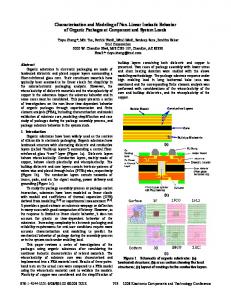
C.J. Taylor and J.A. Noble (Eds.): IPMI 2003, LNCS 2732, pp. 647-659, 2003 @Springer-Verlag Berlin Heidelberg 2003

Nonlinear Estimation and Modeling of fMRI Data using Spatio-Temporal Support Vector Regression Yongmei Michelle Wang1, Robert T. Schultz2, R. Todd Constable1 and Lawrence H. Staib1 1

Department of Diagnostic Radiology; 2 Child Study Center Yale University School of Medicine, New Haven, CT 06520 {[email protected]} Abstract. This paper presents a new and general nonlinear framework for fMRI data analysis based on statistical learning methodology: support vector machines. Unlike most current methods which assume a linear model for simplicity, the estimation and analysis of fMRI signal within the proposed framework is nonlinear, which matches recent findings on the dynamics underlying neural activity and hemodynamic physiology. The approach utilizes spatio-temporal support vector regression (SVR), within which the intrinsic spatio-temporal autocorrelations in fMRI data are reflected. The novel formulation of the problem allows merging model-driven with data-driven methods, and therefore unifies these two currently separate modes of fMRI analysis. In addition, multiresolution signal analysis is achieved and developed. Other advantages of the approach are: avoidance of interpolation after motion estimation, embedded removal of low-frequency noise components, and easy incorporation of multi-run, multi-subject, and multi-task studies into the framework.

1 Introduction Functional magnetic resonance imaging (fMRI) is a noninvasive technique for mapping brain function by the blood oxygenation level dependent (BOLD) effect [23]. In recent years, it has played an increasing role in neuroscience research, and is beginning to become useful clinically as well, for example, in surgical planning. However, the small signal change due to the BOLD effect is very noisy and susceptible to artifacts such as those caused by scanner drift, head motion, and cardio-respiratory effects. Although a task or stimulus can be repeated over and over again, there are limits due to time constraints, learning adaptation of the subjects, etc. Therefore, refined techniques from statistics, biosignal/image processing and analysis are required for accurate detection and characterization of functional activity. The BOLD signal is a complex function of neural activity, oxygen metabolism, cerebral blood volume, cerebral blood flow (CBF), and other physiological parameters. The dynamics underlying neural activity and hemodynamic physiology are believed to be nonlinear [2,21]. Most existing fMRI data analyses assume a linear model, and primarily rely on linear methods or general linear models. As fMRI experiments have grown more sophisticated, the role of nonlinearities has become more important. Statistical evidence that justifies the use of nonlinear analysis for fMRI has

also been provided recently [16]. The feasibility of its application to fMRI data has rarely been shown previous to this work. What makes fMRI analysis challenging are two features peculiar to fMRI. First, fMRI data have intrinsic spatial and temporal autocorrelations [28]. Second, fMRI data tend to have clustered activations. Common approaches either assume spatial independence, or spatially smooth the data with a Gaussian kernel in a preprocessing step. Spatial smoothing enables effective detection of a certain size of clustered activation. However, smoothing may produce a biased estimate by displacing activation peaks and underestimating their height. In order to address this issue, spatial modeling has been proposed [7,13] to take the spatial activation pattern into consideration. Since more powerful tests can be obtained with temporal smoothing due to the improved signal to noise ratio [9], a spatio-temporal linear regression method for fMRI activation detection [15] has recently been developed. This method uses the time series of neighboring voxels together with its own. It has the advantage of modeling the intrinsic spatio-temporal autocorrelations of fMRI data, which is one of the novelties of this work as well. The associated benefits compared to the corresponding voxelwise approaches have also been demonstrated. In general, techniques for analyzing fMRI data can be divided into model-driven, e.g. standard general linear model (GLM) [8], and data-driven methods, e.g. principal component analysis (PCA) [1] or independent component analysis (ICA) [20]. In model-driven methods, a model of the expected response is generated and compared with the data. These methods require prior knowledge of event timing from which an anticipated hemodynamic response can be modeled. Although accurate experimental paradigms are usually available, thorough understanding of the hemodynamic changes that relate neuronal activity to the measured BOLD [23] signal is still under research. Also, for brain responses that are not directly locked to the paradigm, model-driven analysis may not be adequate. Data-driven methods, however, explore the fMRI data statistically without any assumption about the paradigm or the hemodynamic response function. This flexibility is desirable especially where it is difficult to generate a good model; however, there are drawbacks. For example, the assumption implicit in PCA is that different modes are gaussian and uncorrelated, whereas ICA assumes that different modes are nongaussian and independent. In addition, a significance estimate for each component is usually not available. Given the advantages and disadvantages, we propose an approach that merges data-driven methods with prior time course modeling by adjusting a model coefficient. Despite the progress in fMRI analysis, there is still a need for robust and unified statistical analysis methods due to the many limitations with existing techniques, as described above. In this paper, we develop a novel, general and reliable nonlinear approach for fMRI analysis based on spatio-temporal support vector regression so that existing difficulties resulting from noise, low resolution, inappropriate smoothing and modeling can be resolved.

648

2 Methods 2.1 Support Vector Machines (SVM) and Support Vector Regression (SVR) The Support Vector Machine (SVM), introduced by Vapnik [27] and studied by others [26,5], is a new and powerful learning methodology that can deal with nonlinear classification (SVC) and regression (SVR). It is systematic and principled, and has become very popular recently in the machine learning community. The idea of SVR is based on the computation of a linear regression function in a high dimensional feature space where the input data are mapped via a nonlinear function. Here we sketch the ideas behind SVR; a more detailed description of SVR can be found in Smola [26]. Given M input sample points xv1 , xv2 ,K, xvi ,K, xvM , where xvi ∈ ℜ z , and M corresponding scalar output values, y1 , y 2 ,K, yi ,K, y M , the aim is to find an approximation or a regression function of the form: M v v v y = f ( x ) = ∑α i K ( xi , x ) + b

(1)

i =1

to learn this input – output mapping from the set of training examples with high generalizability. The training process of SVR is to find an optimal set of Lagrange multipliers, α i , ∀i ∈ [1, M ] , by maximizing the SVR objective function: M

M

O = −ε ∑ α i + ∑ y i α i − i =1

i =1

M

1 2

M

∑ ∑α α i =1 j =1

i

j

v v K ( xi , x j )

(2)

subject to: 1) linear constraints:

M

∑α i =1

2) box constraint:

i

= 0,

(3)

− C ≤ α i ≤ C , ∀i ∈ [1, M ]

(4) v α i is the Lagrange multiplier associated with each training example xi . ε in Eq. (2) is the insensitivity value meaning that training error below ε is not taken into account as error. C is the tradeoff constant between the smoothness of the SVR function and the total training error. K in Eqs. (1) and (2) is the kernel function. When the approximation function can not be linearly regressed, the kernel function maps training examples from the input space to a high dimensional feature space ℑ by v v x → Φ(x ) ∈ ℑ , in such a way that the function f between the output and the mapped input data points can now be linearly regressed in the feature space. K describes the inner product in the feature space: v v v v K ( xi , x j ) = Φ( xi ) ⋅ Φ( x j )

(5)

There are different types of kernel functions. A commonly used kernel function is the Gaussian radial basis function (RBF):

649

v v  − xv − xv  K ( x i , x j ) = exp 2i σ 2 j    2

(6)

Maximizing the SVR objective function in Eq. (2) by SVR training provides us with an optimum set of Lagrange multipliers, α i , ∀i ∈ [1, M ] . The coefficient, b, of the estimated SVR function in Eq. (1) can be computed by adjusting the bias to pass through one of the given training examples with non-zero α i . With the nonlinear kernel mapping, the regression function in Eq. (1) can be interpreted as a linear combination of the input data in the feature space. Only those input elements with non-zero Lagrange multipliers contribute to the determination of the function. In fact, most of the α i ’s are zero. The training data with non-zero α i are called “support vectors”. Support vectors form a sparse subset of the training data. This type of representation is especially useful for high dimensional input spaces. 2.2 fMRI Data Representation by 4-Dimensional (4D) Spatio-Temporal SVR SVR has recently been applied to system identification, nonlinear system prediction and face detection with good results [11,22,18]. Comparisons of SVR with several existing regression techniques, including polynomial approximation, radial basis functions, and neural networks were carried out in [22]. Initial attempts that directly use SVM have also been achieved for modeling hemodynamic response [3] and for comparing the patterns of fMRI activations to different visual stimuli [10]. However, the application of SVR in the context of fMRI analysis has not yet been exploited and developed. This work is the first one that introduces SVR into fMRI analysis. We formulate fMRI data as spatially windowed continuous 4D functions. That is, the fMRI data is divided into many small windows, such as a 3 × 3 × 3 region within which the entire time series is included. Each input (the training data) within a window is a 4D vector equal to the row, column, slice, and time indices of a voxel. The output is the corresponding intensity. We approximate and recover all training data within the respective windows using SVR. The detailed formulation follows. Let y (u, v, w, t ) be the fMRI signal of voxel [u, v, w]T at a given time point t, where u, v, and w are the respective row, column and slice coordinates of the data. If the 4D fMRI data size is S u × S v × S w × S t , where S t is the total number of time points, the v corresponding input vector x is represented as

v T x = [u, v, w, t ] ,

u ∈ [1, S u ], v ∈ [1, S v ], w ∈ [1, S w ], t ∈ [1, S t ] .

(7)

Within each spatio-temporal window of size M u × M v × M w × S t = M , we have M v v v v input samples x1 , x 2 , K, xi , K, x M , where xvi ∈ ℜ 4 , and the respective scalar output y1 , y 2 ,K , y i ,K , y M . SVR is used to restore the training examples within the window. Local intrinsic spatio-temporal correlations are accounted for during the regression by controlling function smoothness and training error through parameter C (Eq. (4)). In order to compensate for the spatial correlation between neighboring windows, we use

650

spatially overlapped windows (in all three dimensions) so that the recovered intensities over the overlapped voxels are averaged from the corresponding windows. 2.3 Incorporation of Temporal Modeling into Spatio-Temporal SVR Without loss of generality, we assume a simple on-off boxcar function as our model variable, which contains p zeros or ones during each OFF or ON period, and c repetitions or cycles of these two periods. The total number of time points, S t , should be equal to c × 2 p . The resulting boxcar function, m(t), is:

0, if t = 1, K, p; 2 p + 1, K,3 p; K; S t − 2 p + 1, K, S t − p m(t ) =  1, if t = p + 1, K,2 p; 3 p + 1, K,4 p; K; S t − p + 1, K, S t

(8)

where t ∈ [1, S t ] . An additional model entry, based on m(t) in Eq. (8), is added to each input data and makes our SVR a 5-dimensional (5D) regression problem:

v T x = [u, v, w, t , m(t )] ∈ ℜ5

v x (9)

whereas the output is still the corresponding fMRI signal y (u , v, w, t ) . A simple analogy of this model incorporation is not available in traditional signal analysis because fMRI analysis is quite different from conventional systems that are fully characterized by an impulse response. The human brain is a very complicated system: only certain regions of the brain may activate according to the hemodynamic response while many other regions do not. Given the input and output, we need to find out which part of the brain belongs to the hemodynamic response involved region. Fig. 1. General Linear Model regression and boxcar function fitting diagram.

α =

×

+

µ

Voxel time series vector

Design matrix

Parameters

Error vector

The intuitive justification of our modelbased formulation can be achieved by analogy with the General Linear Model (GLM) as it is typically used in fMRI [8]. GLM is given by:

Y = Xβ + e

(10)

where Y is a fMRI data matrix; X is a “design matrix” specifying the time courses of all factors hypothesized to be present in the observed data (e.g., the task reference function, or a linear trend); β is a map of voxel values for each hypothesized factor; and e is a matrix of noise or residual modeling errors. Given this linear model and a design matrix X, the β maps can be found by least squares estimation. The simplest example of the design matrix consists of a boxcar reference function (as in Eq. (8)) and a column vector with all entries constant 1 representing the mean value, without any other hypothesized factors (Fig. 1). In this case, for each voxel, the time series

651

vector is regressed through fitting the boxcar function and the mean value µ (Fig. 1). For this voxel at a give time t, the fitting vector is the corresponding row of the design matrix and can be represented as:

[m(t ), 1]T

(11)

i.e. either [0, 1]T or [1, 1]T . We extend this idea to SVR. Support Vector Machines have very good learning and generalization abilities. As long as we construct the input vectors with the essential features we would like the machine to learn, SVR can capture the complicated relationships (nonlinear or linear) hidden in the training examples. Therefore, for fMRI data representation, in addition to using the indices of the coordinates and time point as input vectors, we also add extra model fitting entries to the input vectors. For the model fitting vector in Eq. (11), the 2nd entry is a constant 1, which is the same for all the input vectors and can be neglected in SVR learning. With the input vector in Eq. (9), we incorporate temporal modeling into the regression. Although the m(t) here is a simple boxcar function, it can be any reference function from prior knowledge about the event timing and hemodynamic response. 2.4 Multiresolution Effects with W-scale

With the above formulation, in order to capture the underlying relationship using SVR for the windowed data and accommodate the differences in scale and training set size, the corresponding entries in the input vector are normalized over training examples within each window. After normalization, we multiply all t i by a coefficient Wscale, and all m(t i ) by a coefficient W-model, whose effects are explained below. We can adjust the effect of temporal scale by varying W-scale, the coefficient for the time indices. Varying W-scale is equivalent to examining the temporal data at different scales. Larger W-scale corresponds to finer temporal resolution. We can restore the time course at multiple resolutions and extract different frequency components by changing W-scale. Many voxel time series in fMRI exhibit low frequency trend components that may be due to aliased high frequency physiological components or drifts in scanner sensitivity. These trends can be removed in a variety of ways. In addition to using a simple high-pass filtering in the temporal domain, a running-lines smoother has been proposed [19] fitting with linear regression (by leastsquares) to the k nearest neighbors of a given point. The approach used by Skudlarski et al. [25] accounts for drift during calculation of the SPM. However, both methods only aim to handle linear trends. In our spatio-temporal nonlinear SVR, with appropriate W-scale (usually relatively small), the low frequency noise can be extracted and removed, and thus achieve nonlinear de-trending. The optimal W-scale for a specific frequency component is expected to be related to the total number of time points, the period of the stimulation, and the data noise level, whose value is currently determined empirically. More rigorous formulation of W-scale determination is one of our future directions, which might also be achieved in the frequency domain through spectrum analysis, etc.

652

2.5 Merging Model-driven with Data-driven through W-model

The coefficient associated with the model index, W-model, determines the degree of influence of the temporal model term and the degree to which the approach is modeldriven. Higher W-model (W-model = 1) is used when reliable temporal models are available. Otherwise, lower or zero W-model is used, and the approach becomes more data-driven. W-model can be interpreted as a model confidence or fitness measure, whose value could be empirically pre-determined as a constant or estimated from regression residual analysis shown below, though extra computation is needed. To arrive at a measure of adequacy of the temporal model, we examine how much of the variation in the response variable is explained by the fitted regression data. We view an observed y i as consisting of two components: observed y = explained by the regressed relation + residual. The differences ( y i − yˆ i ) = (observed response – predicted), or residuals [14], would all be zero in the ideal situation where all the observed points lie exactly on the regressing line, and the y values would be completely v accounted for by the regression on x . We consider the mean of the absolute values of the residuals to be an overall measure of the discrepancy or departure from regression, denoted as D: D =

M

1 M

∑| y i =1

i

− yˆ i | . This discrepancy measure can be used to es-

tablish an appropriate value for W-model. Let the D values calculated from our model-driven (W-model = 1) and data-driven (W-model = 0) methods be D_model and D_data, respectively. We define D_diff = D_data – D_model. For each window, an improved W-model can be estimated according to: 0,  W-model =  D _ diff ,  D _ high − D _ low  1, 

if D _ diff < D _ low

(12)

if D _ low ≤ D _ diff < D _ high if D _ diff ≥ D _ high

where D_high and D_low are high and low threshold values respectively.

3 Experiments and Results1 We validate the approach by using the conventional t-test [17] on our SVR restored fMRI data for activation detection, without additional pre-smoothing or postprocessing. The Gaussian RBF kernel function (Eq. (6)) is used in our experiments with σ set empirically to 0.1. Other SVR parameters are also set empirically: C=1200, ε = 20 (Eqs. (2), (4)). 3.1 Simulated Data

3.1.1 Data Generation

1

For the original color figures in this Section (Figs. 2 - 6), please check web site: http://noodle.med.yale.edu/~wang/Research/ipmi03_fig.html

653

In order to test with access to ground truth, we generate a 2D (spatial size 52 × 63) time series of synthetic data that imitates a single fMRI brain slice in which four regions are activated. Three different amplitudes of activations are added to the gray matter (intensity 180) to simulate weak, medium and strong activations as in real fMRI data. For simplicity, the activations are temporally in the form of a boxcar function, with 6 scans during each off or on period. Note that a more realistic and complicated reference function formed by convolving this boxcar with a Gamma function [4] can also be used, but we expect that the performance would be similar. The total number of time points is 72 (6 cycles). The generated data in Fig. 2(a) is then used as ground truth for comparisons. Simulated noisy data are obtained by adding Gaussian noise, N (0,30 2 ), N (0,40 2 ), N (0,50 2 ), to the ground truth data (see Fig. 2(b) for N ( 0,30 2 ) ). 3.1.2 Effects of W-scale and W-model

For this dataset, the SVR window size used is: 3 × 3 × 3 × 72. Fig. 3 left demonstrates the effects of W-scale by showing the recovered time courses for an activated pixel of the simulated noisy data (Fig. 2(b)) without model fitting (W-model = 0, data-driven). As W-scale increases, higher frequency temporal components are extracted. When Wscale = 5 (Fig. 3(a)) the restored signal captures the low frequency component which can be interpreted as a nonlinear trend. Fig. 3 right demonstrates the effects of varying W-model by showing the recovered time series for the same activated pixel when W-scale = 0, which corresponds to zero frequency (d.c. component). As W-model increases, the temporal models have stronger and stronger effects during the regression and data fitting. For non-activated pixels, the model term barely affects the data regression as long as the gray-level variation at these locations does not happen to match the stimulus cycles. Note that since these are simulated data and no real physiological or neuronal activities are involved, the recovered time courses do not show any lag or undershoots. In fact, the recovered time course accurately restores the ground truth time course (Fig. 3(f)), i.e., the boxcar function. T

Fig. 2. Simulated 2D+T data. Top row: time T vs. spatial axis X; Bottom row: spatial axis Y vs. X.

X (a)

(b)

(c)

(d)

Y

X

(a): Ground truth data; (b): Simulated noisy data, with noise level N (0,30 2 ) ; (c): Restored data by our SVR (W-model = 1); (d): Gaussian smoothed data with s.t.d = 0.5.

3.1.3 Recovered Image and ROC analysis for Activation Detection

The recovered image by our method (W-model = 1) (Fig. 2(c)) accurately restores the ground truth (Fig. 2(a)). The image obtained using Gaussian smoothing of the original noisy data is shown in Fig. 2(d) for comparison. Obviously, our SVR significantly

654

improves the quality of the noisy data. We also applied the t-test for activation detection on i) non-smoothed original noisy data; ii) pre-smoothed data; iii) our SVR recovered data with W-model = 1; iv) our SVR recovered data with W-model determined by Eq. (12), for all three noise levels. Note that for case iv), in Eq. (12), we empirically set D_low = 0 and D_high = 0.015 × minimum(D_model, D_data). The locations and intensities of detected activations can then be compared to the known pattern of added activations to measure the accuracy of detection. We use receiver operating characteristic (ROC) analysis for evaluation. The application of ROC analysis to the analysis of fMRI processing techniques was introduced by Constable et al. [6] and has been used extensively as a tool for objective comparisons of various strategies [25]. The essence of ROC analysis is the comparison of true activation rates (proportion of voxels correctly detected as significant to all voxels with added activations) obtained with different analysis techniques for a given false activation rate (proportion of voxels incorrectly detected as significant to all voxels without added activations). A plot of true activation rate versus false activation rate for different threshold values of a rating scale is called an ROC curve. Under the assumption that the underlying data for true positives and true negative trials form a binormal distribution, the area under the ROC curve can be shown to be the probability that the corresponding analysis technique will correctly identify the true positives. (Average effect of three noise levels)

Fig. 3. Effects on time course with varying W-scale and 2 W-model in our SVR. (Simulated noise level: N (0,30 ) .)

Fig. 4. ROC curves for simulated noisy 2D + T data.

The visual comparison of the ROC curves in Fig. 4 (the average effects of the noisy data at three different noise levels: N (0,30 2 ), N (0,40 2 ), N (0,50 2 ) ) indicates that our SVR approaches outperform the simple t-test yielding larger areas under the ROC curves. Compared with using fixed W-model = 1, determining W-model based on the model fitness / confidence measure (Eq. (12)) leads to further enhancement in activation detection. From the results of the t-test on the original noisy data and presmoothed data, we can see that pre-smoothing improves the detection accuracy.

655

3.2 Real fMRI Data

We also applied the proposed approach to a block-design cognitive fMRI experiment [24], examining social attribution to geometric animations. T2*- weighted images are acquired using a single shot echo planar sequence. The pulse sequence is TR = 1500ms, TE = 60ms, flip angle= 60 o , NEX=1, in plane voxel size = 3.125 × 3.125mm2. 14 coronal slices are collected and are 10mm thick (skip 1mm). Corresponding T1-weighted structural images of the same thickness are collected in the same session (TR=500, TE=14, FOV=200mm, 256 × 192mm matrix, 2NEX). The first four volumes of fMRI time series are discarded to discount T1 saturation effects. We have examined this dataset for a visuospatial task from one subject and one run. The window size we used is 3 × 3 × 1 × 160, where 160 is the total number of time points. We did not use an isotropic window since the voxel shape is not cubic. The 3 × 3 × 1 window covers a brain region whose physical size is almost isotropic (9.4 × 9.4 × 10mm3). Visual comparisons in Fig. 5 with t-test results (on pre-smoothed data with empirically optimal FWHM=6.25mm) reveal that our SVR approach (Wmodel = 1) leads to: greater spatial extent and statistical significance in the intraparietal sulcus (IPS) with potentially better delineation and localization of the underlying spatial activation. Note: at the top of each slice in Fig. 5 are the respective p-value and t-value for threshold. When the same t-threshold used for SVR (t > 7.8) is used for the t-test, no activations are detected. For t-test in Fig. 5(c), we intentionally further decrease the t-threshold to t > 2.3 and try to detect more IPS activation regions, which, however, leads to a more blurred spatial extent rather than precisely localized spatial activation as in Fig. 5(a), as well as some false activations. The associated time course for an activation voxel from our SVR method for this data is shown in Fig. 6. (a): by SVR

(b): by t-test

(c): by t-test

( p 7.8 ) ( p 4.2 ) ( p 2.3 )

Fig. 5. Results comparison for real fMRI data from a visuospatial task. (Color activation maps.)

Fig. 6. Time courses of an activation voxel for the real fMRI data in Fig. 5.

4 Conclusions and Discussions From a signal processing viewpoint, fMRI activation detection is a problem of nonlinear spatio-temporal system identification. We have presented a novel regression model involving spatio-temporal correlations using support vector regression. Many pre-processing procedures, such as smoothing, de-trending, and interpolation after motion estimation, required by other methods, are embedded within this unified framework. Experimental results on both simulated and real fMRI data revealed its effectiveness. The approach meets the need for reliable and sensitive fMRI signal analysis. A few comments on the particulars of our method are discussed below.

656

In this paper, primarily, we discussed the method using block-design paradigms. However, the approach can be applied to event-related experiments as well. The exploration of the framework on event-related fMRI data is one of our future directions. The size of the spatial window within which we perform SVR is empirically set as 3 × 3 × 3 or 3 × 3 × 1. This not only ensures that the included area covers a brain region whose physical size is almost isotropic, but also allows for some spatial continuity while limiting the likelihood of heterogeneous activation within the same window. Correction for head motion involves rigid-body transformation estimation and resampling. Due to the thick image slices typical of fMRI, intensity interpolation, required during the resampling process, can introduce significant artifacts [12]. With our SVR approach, interpolation after motion estimation is avoided due to the use of continuous variables for both the input vectors and output scalar. The spatial coordinates and time indices used in the SVR learning can be any continuous (floating point) value. This advantage is not available for other methods. The ability of SVR to handle high dimensional input data makes it ideally suited for extensions to multi-run, multi-subject and multi-task studies. Our SVR formulation allows easy incorporation of data from multiple sessions by expanding the input vectors and analyzing the data over multiple runs and subjects together. Similar to the spatial and temporal indices, now we would have two additional dimensions for run and subject indices. This technique would account for between-run and betweensubject variability with likely increased statistical significance in activated regions. The multi-task problem can also be solved in a similar way i) using only one model function as that in Eq. (8), with 0 representing rest, and 1 representing all the designated tasks; or ii) expanding the input vectors with each function representing a specific task (i.e. 1), versus true rest and all other tasks (i.e. 0). In addition to exploring the above described issues, our future work also includes temporal model estimation from our SVR restored data without assuming a specific shape of the hemodynamic response function, combining this hemodynamic modeling to improve the specificity and sensitivity of fMRI signal detection, comparison with the General Linear Model for activation detection, incorporating spatial models such as information about the configuration of the activation regions and anatomic prior knowledge into the framework, as well as further validation.

Acknowledgments This work was partially supported by NIH grant EB000311. The authors would like to thank the anonymous reviewers for comments that considerably improved the quality of this paper.

References 1. Backfriender, W., Baumgartner, R. Stamal, M., Moser, E., Bergmann, H.: Quantification of intensity variations in functional MR images using rotated principal components. Physics in Medicine and Biology 41 (1996) 1425-1438 2. Birn, R.M., Saad, Z.S., Bandettini, P.A.: Spatial heterogeneity of the nonlinear dynamics in the fMRI BOLD response. Neuroimage 14 (2001) 817-826

657

3. Boulanouar, K., Roux, F., Celsis, P.: Modeling brain hemodynamic response in functional MRI using vector support method. In: Cognitive Neuroscience Society Annual Meeting (Abstract) (2001) 4. Boynton, G.M., Engel, S.A. Glover, G.H., Heeger, D.J.: Linear systems analysis of functional magnetic resonance imaging in human V1. J. Neuroscience 16 (1996) 4207-4221 5. Collobert, R., Bengio, S.: SVMTorch: Support vector machines for large-scale regression problems. Journal of Machine Learning Research 1 (2001) 143-160 6. Constable, R.T., Skudlarski, P., Gore, J.C.: An ROC approach for evaluating functional brain MR imaging and postprocessing protocols. Magnetic Resonance in Medicine 34 (1995) 57-64 7. Descombes, X., Kruggel, F., von Cramon, D.Y.: fMRI signal restoration using a spatiotemporal Markov random field preserving transitions. Neuroimage 8 (1998) 340-349 8. Friston, K.J., et. al.: Statistical parametric maps in functional imaging: A general linear approach. Human Brain Mapping 2 (1995) 189-210 9. Friston, K.J., Holmes, A.P., Poline, J-B, Grasby, P.J., Williams, S.C.R., Frackowiak, R.S.J.: Analysis of fMRI time-series revisited. Neuroimage 2 (1995) 45-53 10. Golland, P., et. al.: Discriminative analysis for image-based studies. In: Intl. Conf. on Medical Image Computing and Computer-Assisted Intervention (2002) 508-515 11. Gretton, A., Doucer, A., Herbrich, R., Rayner, P.J.W., Scholkopf, B.: Support vector regression for black-box system identification. In: IEEE Workshop on Statistical Signal Processing (2001) 341-344 12. Grootoonk, S., Hutton, C., Ashburner, J., Howseman, A.M., Josephs, O., Rees, G., Friston, K.J., Turner, R.: Characterization and correction of interpolation effects in the realignment of fMRI time series. Neuroimage 11 (2000) 49-57 13. Hartvig, N.V., Jensen, J.L.: Spatial mixture modeling of fMRI data. Human Brain Mapping 11 (2000) 233-248 14. Johnson, R.A., Bhattacharyya, G.K.: Statistics: Principles and Methods. John Wiley & Sons, Inc. (2001) 15. Katanoda, K., Matsuda, Y., Sugishita, M.: A spatio-temporal regression model for the analysis of functional MRI data. Neuroimage 17 (2002) 1415-1428 16. Laird, A.R., Rogers, B.P., Meyerand, M.E.: Investigating the nonlinearity of fMRI activation data. In: Proc. Second Joint EMBS / BMES Conference (2002) 23-26 17. Lang, N.: Statistical procedures for functional MRI. In: Moonen, C, Bandettini, P. (eds.): Functional MRI. Springer-Verlag (1999) 301-355 18. Li, Y., Gong, S., Liddell, H.: Support vector regression and classification based multi-view face detection and recognition. In: Proc. Fourth IEEE Intl. Conf. on Automatic Face and Gesture Recognition (2000) 300-305 19. Marchini, J.L., Ripley, B.D.: A new statistical approach to detecting significant activation in functional MRI. Neuroimage 12 (2000) 366-380 20. McKeown, M., Makeig, S., Brown, G., Jung, T., Kindermann, S., Bell, A., Sejnowski, T.: Analysis of fMRI data by blind separation into independent spatial components. Human Brain Mapping 6 (1998) 160-188 21. Miller, K.L., Luh, W.M, Lie, T.L., Martinez, A., Obata, T., Wong, E.C., Frank, L.R., Buxton, R.B.: Nonlinear temporal dynamics of the cerebral blood flow response. Human Brain Mapping 13 (2001) 1-12 22. Mukherjee, S., Osuna, E., Girosi, F.: Nonlinear prediction of chaotic time series using support vector machines. In: Proc. IEEE Workshop on Neural Networks and Signal Processing Vol. VII (1997) 511-520 23. Ogawa, S., Lee, T.M., Nayak, A.S., Glynn, P.: Oxygenation-sensitive contrast in magnetic resonance image of rodent brain of high magnetic fields. Magnetic Resonance in Medicine 14 (1990) 68-78

658

24. Schultz, R.T., et. al.: The role of the fusiform face area in social cognition: Implications for the pathobiology of autism. Phil. Trans. of the Royal Society, Series B, 358 (2003) 415-427 25. Skudlarski, P., Constable, R.T., Gore, J.C.: ROC analysis of statistical methods used in functional MRI: Individual subjects. Neuroimage 9 (1999) 311-329 26. Smola, A.J., Scholkopf, B.: A Tutorial on Support Vector Regression. NeuroCOLT Technical Report NC-TR-98-030, Royal Holloway College, University of London, UK (1998) 27. Vapnik, V.N., Statistical Learning Theory. John Wiley & Sons, New York (1998) 28. Zarahn, E., Aguirre, G.K., D’Esposito, M.: Empirical analyses of BOLD fMRI statistics. I. Spatially unsmoohed data collected under null-hypothesis conditions. Neuroimage 5 (1997) 179-197

659