Jenghwa Chang, Harry L. Graber, and Randall L. Barbour. Department of Pathology and Department of Biophysics, State University of New York Health Science ...
Zhu et al.
Vol. 14, No. 4 / April 1997 / J. Opt. Soc. Am. A
799
Iterative total least-squares image reconstruction algorithm for optical tomography by the conjugate gradient method Wenwu Zhu,* Yao Wang, and Yuqi Yao* Department of Electrical Engineering, Polytechnic University, Brooklyn, New York 11201
Jenghwa Chang, Harry L. Graber, and Randall L. Barbour Department of Pathology and Department of Biophysics, State University of New York Health Science Center, Brooklyn, New York 11203 Received May 3, 1996; accepted October 14, 1996; revised manuscript received October 16, 1996 We present an iterative total least-squares algorithm for computing images of the interior structure of highly scattering media by using the conjugate gradient method. For imaging the dense scattering media in optical tomography, a perturbation approach has been described previously [Y. Wang et al., Proc. SPIE 1641, 58 (1992); R. L. Barbour et al., in Medical Optical Tomography: Functional Imaging and Monitoring (Society of Photo-Optical Instrumentation Engineers, Bellingham, Wash., 1993), pp. 87–120], which solves a perturbation equation of the form WDx 5 DI. In order to solve this equation, least-squares or regularized least-squares solvers have been used in the past to determine best fits to the measurement data DI while assuming that the operator matrix W is accurate. In practice, errors also occur in the operator matrix. Here we propose an iterative total least-squares (ITLS) method that minimizes the errors in both weights and detector readings. Theoretically, the total least-squares (TLS) solution is given by the singular vector of the matrix [WuDI] associated with the smallest singular value. The proposed ITLS method obtains this solution by using a conjugate gradient method that is particularly suitable for very large matrices. Simulation results have shown that the TLS method can yield a significantly more accurate result than the least-squares method. © 1997 Optical Society of America [S0740-3232(97)01004-1] Key words: image reconstruction, total least squares, medical optical tomography, conjugate gradient method.
1. INTRODUCTION Over the past few years, research on medical optical tomography has progressed rapidly. Interest remains high because the method appears to offer several important advantages over other established imaging modalities. These include use of nonionizing sources and highly sensitive detectors, the ability to monitor situations and events critical to sustaining life (e.g., tissue oxygenation), and the availability of compact, low-cost instrumentation that can be made portable. In addition, through use of optical fibers, measurements can be performed simultaneously with the collection of imaging data from other modalities. This avoids registration errors, which, as recently shown for magnetic resonance imaging data,1 can greatly facilitate the computation and the stability of the optical reconstructions. We have previously described an iterative perturbation approach for reconstructing the optical properties of a random scattering medium using different source conditions [e.g., continuous wave (cw) and time-resolved data].2–5 In each case this requires the solution of a linear perturbation equation at each iteration of the form WDx 5 DI,
(1)
where Dx is a vector of differences in the optical properties (absorption or scattering) between a reference and a 0740-3232/97/040799-09$10.00
test medium, DI is a vector of changes in detector readings between the two media, and W is a matrix of weights describing the influence of each volume element (voxel) on the detector readings. The elements of W essentially are the derivatives of the detector readings with respect to the absorption or scattering coefficients in the reference medium. To solve the linear perturbation equation, several iterative algorithms have been developed, including projection onto convex sets,2 a conjugate gradient descent (CGD) method,2 a multigrid method,2 a layer-stripping scheme,4,5 and wavelet-based regularized least-squares.6 These methods are all based on the least-squares (LS) formulation, which finds a solution that best fits the measurement Dx while assuming that the weight matrix W is accurate. In practice, the latter assumption is not accurate, and corrections to W must be made in order to compute an accurate solution. Three approaches come to mind. One would be to adopt recursive iterative methods (Newton type) that seek to solve the linear equation by updating alternately the forward and inverse problem solutions. Several groups,7 including ours,8 have reported some success with this scheme. This includes media having complex backgrounds (e.g., magnetic resonance maps1) and analysis of experimental data.9 The difficulty with this is that, even for two-dimensional problems, the computational burden can become undesirable, particularly if multiple updates are required. Another © 1997 Optical Society of America
800
J. Opt. Soc. Am. A / Vol. 14, No. 4 / April 1997
Zhu et al.
approach would be to update W by solving a nonlinear equation relating DI to Dx, as has been recently described by Graber et al.10 This has the potential advantage that corrections to W can be made by evaluating an analytical expression, thereby avoiding the computational expense of updating the forward problem. As the expression derived is only an approximation, it seems likely that some, perhaps fewer, updates will be needed. A third approach, adopted in this paper, is to compute solutions to Eq. (1) that minimize errors in both W and DI. Methods of this type have been applied to other imaging problems and are referred to as the total leastsquares (TLS) method. For example, Justice and Vassiliou applied the TLS approach to geophysical diffraction tomography.11 A regularized constrained TLS was proposed by Mesarovic´ et al.12 for dealing with image restoration problems, where noise in the point-spread function (the convolution operator) H and the data y are linearly dependent (algebraically correlated). Singular-valuedecomposition- (SVD-) based TLS was employed by Li et al.13 in phased array imaging, where it is assumed that noise in H and y are independent. While seemingly effective, the TLS solution obtained by SVD has computational limitations for large-scale systems. This is because the SVD computation needs O(N 3 ) multiplications, where N is the length of vector x. Since computation is a major concern in optical tomography, an iterative TLS (ITLS) approach is developed here. The TLS solution is obtained by minimizing a Rayleigh-quotient function with use of the conjugate gradient (CG) method, which is suitable for large-dimension data. The arrangement of this paper is as follows. Section 2 reviews the perturbation model for optical diffusion tomography derived based on the transport equation and the diffusion equation, respectively. Section 3 presents the TLS formulation. Section 4 describes how to solve the TLS solution iteratively by using the CG method. Section 5 shows simulation results of the proposed method. Finally, Section 6 summarizes the main results and suggests directions for future study.
tion V and ma (r, V) represents macroscopic angular absorption cross section at position r in the direction V. Symbolically, Eq. (2) can be expressed as Lu 5 s,
(3)
where L is an integrodifferential operator. Let the optical properties and the angular intensity be perturbed from those of a reference medium. Then the transport equation becomes ~ L 1 DL !~ u 1 Du ! 5 s,
(4)
or LDu 5 s 2 Lu 2 DLu 2 DLDu 5 2DLu 2 DLDu. (5) If the DLDu term can be ignored, then we obtain LDu 5 2DLu.
(6)
That means that if u is the solution satisfying the boundary conditions with source s, then Du is the solution satisfying the same boundary conditions with source s 8 5 2DLu.
(7)
Let G(r1 , V1 ; r2 , V2) be the Green’s function satisfying the transport equation for the reference medium, and assume that only absorption cross sections are perturbed. We further assume that the source density is s(r, V) 5 d (r 2 rs , V 2 V s ) and that the optical properties of the medium are isotropic, i.e., m a (r, V) 5 m a (r) and m s (r, V) 5 m s (r). Under these assumptions the solution of the perturbation equation is given by Du ~ rd , V d , rs , V s ! 5
E
V
D m a ~ r8 ! w a ~ rd , V d , rs , V s ; r8 ! d3 r8 ,
(8)
where w a ~ rd , V d , rs , V s ; r8 !
2. PERTURBATION MODEL
5
A. Perturbation Equation Derived Based on the Transport Equation Under cw illumination the photon density in a scattering medium is governed by a radiation transport equation14: 2V • ¹u ~ r, V ! 2 m t ~ r, V ! u ~ r, V ! 1
E
m s ~ r, V 8 → V ! u ~ r, V 8 ! dV 8 1 s ~ r, V ! 5 0,
E
4p
G ~ r8 , V 8 ; rs , V s ! G ~ r8 ,2V 8 ; rd ,2V d ! dV 8
(9)
is called the weight function. It indicates the influence or the importance of absorption at r8 to the source– detector pair at (rs , V s ) and (rd , V d ). In the above equation (rs , V s ) and (rd , V a ) are the source location and direction and the detector location and direction, respectively.
(2)
where V represents the direction unit vector, u(r, V) represents photon angular intensity at r with direction V, s(r, V) represents angular source density at r with direction V, m s (r, V 8 → V) represents macroscopic angular scattering cross section at r from direction V8 into direction V, and m t (r, V) 5 m s (r, V) 1 m a (r, V) represents macroscopic angular total cross section at position r in the direction V, where ms (r, V) represents macroscopic angular scattering cross section at position r in the direc-
B. Perturbation Equation Derived Based on the Diffusion Model In media having high albedo (e.g., tissue at near-infrared wavelength), the following diffusion equation provides a good approximation to the transport equation7: ¹ • @ D ~ r! ¹u ~ r!# 2 m a ~ r! u ~ r! 5 2S ~ r! ,
(10)
where D 5 1/3( m a 1 m 8s ) is the diffusion coefficient, m 8s is the equivalent isotropic scattering cross section, and S is the source term.
Zhu et al.
Vol. 14, No. 4 / April 1997 / J. Opt. Soc. Am. A
From the above equation we can obtain the following integral equation: Du ~ rd , rs ! 5
E
V
D m a ~ r8 ! w a ~ rd , r s ; r 8 ! d3 r8 ,
801
Here i•i2 denotes the Euclidean norm. Once EDI is found, Dx is easily determined by solving the compatible equation
(11)
WDx 5 DI 1 EDI .
(17)
It is known that the solution of the above LS problem satisfies the normal equation
with w a ~ rd , rs ; r8 ! 5 G ~ rd 2 r8 ! G ~ rs 2 r8 ! ,
(12)
where G is the Green’s function for the reference medium, satisfying ¹ • @ D ~ r! ¹G ~ r 2 rs !# 2 m a ~ r! G ~ r 2 rs ! 5 2d ~ r 2 rs ! , (13) where D(r) and ma (r) are the diffusion coefficient and the absorption cross section for the reference medium, respectively. C. Image Reconstruction by Solving the Discretized Perturbation Equation Equations (8) and (11) are the perturbation equations in the continuous domain. By discretizing the domain into N small voxels, we can approximate them in the following matrix form: WDx 5 DI,
(14)
where Dx 5 @ Dx 1 ,...,Dx N # T (where T denotes transpose), DI 5 @ DI 1 ,...,DI M # T, and W 5 @ W mn # M3N . The variable Dx n 5 D m a (rn ) represents the absorption perturbation at the voxel located at n, DI m 5 Du(rd m , rs m ) represents the detector reading for the mth source–detector pair located at rs m and rd m , respectively, and W mn 5 w a (rd m , rs m ; rn ) d v is the weight describing the influence of voxel n on source–detector pair m, where d v is the volume of a voxel. The absorption imaging problem (inverse problem) can be stated as follows: For a chosen set of source–detector pairs, given the perturbed detector reading DI and the precalculated weight matrix W from the forward problem, find the perturbation of the macroscopic absorption cross section Dx of the target medium. In general, the perturbation equation is both underdetermined and ill conditioned. The underdeterminedness arises in situations in which the number of detector readings, M, is less than the number of unknowns, N. Even if M > N, the matrix W can be rank deficient, which also leads to an underdetermined system. The cause of the ill conditioning is that W contains many nearly zero columns. Very small variations in DI can result in very large deviations in Dx.
3. TOTAL LEAST-SQUARES FORMULATION In general, when M . N, the perturbation equation is incompatible because of errors in both W and DI. In the conventional LS solution we assume that the measurement DI is noisy but that the weight matrix W is exact, and we seek a correction vector EDI to DI such that we minimize i EDIi 2 ,
(15)
subject to DI 1 EDI P Range~ W! .
(16)
WTWDx 5 WTDI.
(18)
In reality, as described in Section 1, the weight matrix W may also be erroneous and should be corrected. In the TLS approach we try to find a correction matrix EW to W, in addition to EDI so that we minimize i EWu EDIi F ,
(19)
subject to DI 1 EDI P Range~ W 1 EW! .
(20)
Here i•iF denotes the Frobenius norm, which is defined as i Ei F 5 @ ( m ( n (E mn ) 2 # 1/2. After EW and EDI are found, then any DI satisfying ~ W 1 Ew! Dx 5 DI 1 EDI
(21)
is said to be the TLS solution. The TLS solution to an incompatible linear equation was first described by Golub and Van Loan.15 The problem described by Eqs. (19) and (20) can be restated as minimize i Ei F ,
(22)
subject to ~ A 1 E! q 5 0,
(23)
where A 5 @ Wu DI# , q5
E 5 @ Ewu EDI# ,
(24)
S D
Dx . 21
Golub and Van Loan showed that, if Rank(A) 5 N 1 1, the TLS solution is related to the right singular vector vN11 of A associated with the smallest singular value s N11 , under the condition that s N . s N11 and v N11, N11 Þ 0, where sN represents the Nth largest singular value and v N11, N11 is the last component of the singular vector ˜ N11 vN11 . Let vN11 5 @ ˜vN11 T v N11, N11 # T, where v represents the subvector containing the first N components of vN11 . Then the TLS solution is Dx ˜ N11 . 5 (1/v N11, N11 )v For rank-deficient systems the minimum Frobenius norm solution is x N11 N11 v N11, i ˜vi / ( i5p11 v N11, i 2 , where s p . s p11 5 2( i5p11 5 ••• 5 s N11 5 0 and vi 5 @ ˜vi T v N11,i # T. One way to obtain the TLS solution is by SVD of A.15 However, the SVD-based TLS algorithm can become computationally prohibitive for large-scale systems.13,16 In this paper we adopt an iterative scheme that is more suitable for large-scale problems. It has been shown17 that the constrained minimization problem in requirements (22) and (23) is equivalent to the following minimization problem: minimize F ~ q! 5
qTATAq qTq
,
(25)
which in turn is equivalent to finding the eigenvector q associated with the smallest eigenvalue of ATA.17 The function F(q) is called the Rayleigh quotient. The mini-
802
J. Opt. Soc. Am. A / Vol. 14, No. 4 / April 1997
Zhu et al.
mal value of F(q) is in fact equal to the minimal perturbation that satisfies Eq. (21), which in turn equals the minimal singular value, i.e., min(iEi F 2 ) 5 min@F(q) # . In the following we describe a CG method for the minimization of F(q).
P d ~ k ! 5 ^ p~ k ! , p~ k ! & .
(36)
In the above equations ^ x,y& 5 x y represents the inner product of x and y. At time k 1 1 the new search direction is chosen as T
p~ k 1 1 ! 5 r~ k 1 1 ! 1 b ~ k ! p~ k ! ,
(37)
4. CONJUGATE GRADIENT METHOD FOR TOTAL LEAST SQUARES
and the residue r(k 1 1) is given by
In most reported studies the TLS problem is solved by SVD.13,16,18 In general, the SVD calculation needs O(L 3 ) multiplications, where L is the length of vector q. Therefore the SVD-based method is not suitable for large-scale systems. A recursive TLS algorithm was first used by Davila.19 There the generalized eigenvector q was updated with a correction vector chosen as a Kalman filter gain vector, and the scalar (step size) was determined by minimizing the Rayleigh quotient [requirement (25)]. When the underlying linear equation originates from a one-dimensional linear convolution operation, this algorithm requires only O(L) multiplications per iteration.19 Bose et al.20 applied recursive TLS to reconstruct highresolution images from undersampled low-resolution noisy multiframes. In this case the convolution operator corresponds to two-dimensional convolution operation, and the algorithm requires O(L 2 ) multiplications per iteration. In the perturbation equation considered here, the matrix W does not correspond to a convolution operation. Our goal is to find an algorithm that is suitable for very large matrices of arbitrary structure. Toward this goal the CG method originally developed for other applications21,22 has been applied here. Although the CG method requires O(L 2 ) multiplications per iteration, it is well known that the CG method converges very fast and is particularly suitable for large matrices. As stated above, the TLS solution can be obtained by minimizing the Rayleigh quotient in requirement (25). Let q(k) represent the solution at the kth iteration. The CG algorithm updates q by successive approximation:
In our implementation the method for choosing b (k) is slightly different from that used in Ref. 21. We use the method developed by Fletcher and Reeves,24 also described by Yang et al.22 The b (k) is chosen as
q~ k 1 1 ! 5 q~ k ! 1 a ~ k ! p~ k ! ,
(26)
where a (k) is chosen to reach the minimum of F(q) in the direction p(k). Following Shavitt et al.,23 it can been shown that a (k) is always real and satisfies D @ a ~ k !# 2 1 B a ~ k ! 1 C 5 0.
r~ k 1 1 ! 5 l ~ k ! q~ k 1 1 ! 2 ATAq~ k 1 1 ! .
b ~ k ! 5 ^ r~ k 1 1 ! , r~ k 1 1 ! & / ^ r~ k ! , r~ k ! &
(38)
(39)
T
to make the direction vectors p(k) A A-conjugate, i.e.,
^ ATAp~ k ! , p~ k 1 1 ! & 5 0.
(40)
The convergence criterion that we use is u @ l(k 1 1) 2 l(k)]/l(k) u , 1023 ; 1024 . The initial solution q(0) is set to a vector in which all elements except the last are 0 and the last element is set to 1.
5. SIMULATION RESULTS To compare the LS and ITLS approaches, we have attempted reconstructions of two test media. One was a three-layer medium; the other was a cylindrical phantom. Only cw measurement has been considered, although the ITLS can be equally applied to other source conditions. The LS solution was obtained by the CGD algorithm.1 A. Three-Layer Medium We first present reconstruction results for the three-layer medium. The medium is 10 mean-free-path (mfp) thick and is composed of three layers located at depths 0–3, 3–7, and 7–10 mfp. The macroscopic total cross section is constant throughout the slab. The absorption cross section of the first and third layers is 1% of the total, and that of the middle layer is 5%. Scattering is isotropic. Figure 1 shows the geometry of the illumination and de-
(27)
Among the two possible solutions of Eq. (27), the one that yields the smaller value of F(q) is given by
a ~ k ! 5 ~ 2B 1
AB 2 2 4CD ! / ~ 2D ! ,
(28)
where D 5 P b~ k ! P c~ k ! 2 P a~ k ! P d~ k ! ,
(29)
B 5 P b~ k ! 2 l ~ k ! P d~ k ! ,
(30)
C 5 P a~ k ! 2 l ~ k ! P c~ k ! ,
(31)
l ~ k ! 5 ^ Aq~ k ! , Aq~ k ! & ,
(32)
P a ~ k ! 5 ^ Aq~ k ! , Ap~ k ! & ,
(33)
P b ~ k ! 5 ^ Ap~ k ! , Ap~ k ! & ,
(34)
P c ~ k ! 5 ^ p~ k ! , q~ k ! & ,
(35)
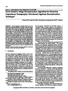
Fig. 1. Position and orientation of detectors about the source. The source is placed in the center. The open circles and the crosses indicate positions of detectors that are inclined 10° and 80° from the normal, respectively. The small solid circles indicate positions where measurements are made in both orientations. The grid size is 3 mfp 3 3 mfp.
Zhu et al.
Fig. 2. Cross section of the original three-layer medium. The darkest gray level represents Dxmax , the maximum value of Dx. Here Dxmax 5 5.0 3 1024 .
tection scheme used. Figure 2 shows the original threelayer medium. One source was employed, and responses of detectors located on the same side as the source (i.e., backscattering only) were computed either by using Monte Carlo simulations (simulated data) or based on the perturbation equation (calculated data). In both cases the weight functions used were calculated by using Monte Carlo simulations.25 To enhance detector discrimination, we employed two different detector orientations: a grazing angle of 10° with respect to the surface and a nearnormal angle of 80° with respect to the surface. The medium was discretized into ten slices, each 1 mfp thick. There were 40 detector readings and ten unknowns, so the problem was overdetermined. The weight functions were calculated for both a homogeneous 10-mfp slab and the actual three-layer medium. These two sets of weights will be referred to as half-space weights and three-layer weights, respectively. Two sets of readings were used: One was calculated from Eq. (1) by using the three-layer weights, and the other one was obtained from Monte Carlo simulations. Four experiments have been conducted. The purpose of the first experiment was to evaluate the ITLS reconstruction algorithm in an ideal situation. The calculated data and three-layer weights were used. Gaussian white noise was added to both the data and the weights. The noise levels tested were 0.1%, 0.2%, and 1% in the detector readings and 0.001%, 0.002%, and 0.01% in the weights. Here the noise level is defined as the ratio of noise standard deviation to the mean of the signal. Each column in the weight matrix and the data column was scaled by the noise standard deviation in this column, so that the noise added to the augmented matrix A has the same variance
Vol. 14, No. 4 / April 1997 / J. Opt. Soc. Am. A
803
in each column. This is required for the TLS-type algorithm to work well. Once the solution for this scaled system was obtained, the final solution was then derived by scaling back with use of the same factors. The reconstruction results obtained by LS and ITLS are shown in Fig. 3. The displayed images (i.e., the image of Dx) are all normalized, so that the maximum value in Dx in each case is represented by the same darkness level. It can be seen that the LS algorithm begins to break down as the noise level increases beyond 1%, while ITLS yields a quite consistent and accurate result under all noise levels. This result was as expected, because the noise in both the weights and the data were truly identically and independently distributed. The second experiment was implemented by using the same data set [i.e., data calculated from Eq. (1) with three-layer weights] but with half-plane weights in W. LS and ITLS methods were used to reconstruct the images of the medium; the reconstruction results are illustrated in Figs. 4(a) and 4(b), respectively. In this case the noise in the weight matrix was not white but has a certain structure. The weights for voxels in the upper slices were likely to be underestimated, while those in the lower slices were overestimated. Even in this case the TLS algorithm gave a fairly accurate result, significantly better than that of the LS method. In the third experiment simulated detector readings by Monte Carlo methods and the three-layer weights were used. The reconstruction results obtained by LS and ITLS methods are shown in Figs. 5(a) and 5(b), respectively. In this case the errors in weights and data by Monte Carlo calculations were approximately independent and identically distributed. The noise levels were fairly low because our Monte Carlo simulations were done with a very high precision. In this case the LS algorithm gave a reasonably good result but not as accurate as that of the ITLS. Both correctly identified the transition from the first to the second layer. The last experiment was conducted by using simulated detector readings and half-plane weights. The reconstruction results by the LS and ITLS approaches are illustrated in Figs. 6(a) and 6(b), respectively. In this case, as in experiment 2, the noise in the weight matrix
Fig. 3. Reconstruction results with use of the three-layer weight function and calculated data. Images in (a), (b), and (c) are the LS reconstruction results under noise levels 0.1%, 0.2%, and 1% in detector readings and 0.001%, 0.002%, and 0.01% in weights, respectively. The maximum reconstruction values are Dxmax 5 6.8 3 1024 , 6.7 3 1024 , and 1.9 3 1023 . Images in (d), (e), and (f) are the ITLS reconstruction results under the corresponding noise levels, with Dxmax 5 5.6 3 1024 , 5.6 3 1024 , and 5.8 3 1024 , respectively.
804
J. Opt. Soc. Am. A / Vol. 14, No. 4 / April 1997
Fig. 4. Reconstruction for the three-layer medium with use of the half-space weights and calculated data: (a) LS reconstruction result by the CGD method, with Dxmax 5 8.7 3 1023 ; (b) ITLS reconstruction result, with Dxmax 5 3.9 3 1024 .
Fig. 5. Reconstruction for the three-layer medium with use of the three-layer weights and simulated data: (a) LS reconstruction result, with Dxmax 5 8.4 3 1023; (b) ITLS reconstruction result, with Dxmax 5 8.4 3 1023 .
Zhu et al.
B. Cylindrical Rod The second test medium was an infinite medium with an embedded cylindrical rod positioned in either a centered or an off-center location with respect to a circular ring of the detectors. A ring of sources and detectors was placed around the rod, as shown in Fig. 7. In the first experiment a 1-cm-diameter rod was placed in the center of the ring. The rod was homogeneous, with absorption and m a 5 0.05 cm21 and ms scattering coefficients 5 10 cm21 . The properties of the background medium were m ba 5 0.02 cm21 and m bs 5 10 cm21 . A total of 16 sources and 16 detectors were evenly spread about the rod in a ring geometry having a diameter of 8 cm (see Fig. 7). Solution to the forward problem was accomplished by analytically solving the diffusion equation by using the normal-mode-series method described by Yao et al.26 In the second experiment a 1.5-cm-diameter rod was placed at an off-center position with respect to the source and detector ring. The rod had a nonhomogeneous absorption distribution, following a sinusoidal pattern (one positive cycle only). The forward solution in this experiment was obtained by a multigrid finite-difference solver, described in Ref. 27. The absorption properties (actually, the perturbation from the background) in a 10-cm 3 10-cm square region enclosing the source and detector ring were reconstructed by using the LS and ITLS methods. This region was discretized to 32 3 32 elements. So the problem is underdetermined. To compare LS and ITLS algorithms, we added white Gaussian noise with a constant variance to both the weights and the detector readings. The noise level was 3% for the detector reading and 0.01% for the weights. Although the average noise level in weights was very small, the actual degradation of weights in some locations was very large. This is because the weights have a very large dynamic range. Figure 8 shows the histogram of noise levels in weights on a log scale. Figure 9 shows a
Fig. 6. Reconstruction for the three-layer medium with use of the half-space weights and simulated data: (a) LS reconstruction result, with Dxmax 5 6.5 3 1021 ; (b) ITLS reconstruction result, with Dxmax 5 1.7 3 1023 .
was not white. Although the result of LS was qualitatively similar to that in experiment 3 [Fig. 5(a)], they were very different quantitatively. The absorption strength was significantly overestimated in those images. With ITLS the absorption strength was overestimated in the upper slices. This was as expected, because the weights there were underestimated. One interesting observation is that the ITLS algorithm yielded a smoother reconstruction than that of the LS algorithm in all four experiments, more clearly indicating the actual threelayer structure. The images reconstructed by the LS algorithm, on the other hand, often contained spurious peaks and valleys.
Fig. 7. Source–detector configurations for the cylindrical rod computation.
Zhu et al.
Vol. 14, No. 4 / April 1997 / J. Opt. Soc. Am. A
805
10(d), 10(e), and 10(f) show similar results for the offcenter case. It can be seen that ITLS yields significantly better reconstruction results than those from LS. For both LS and ITLS the simulation results are obtained with 5000 iterations. One iteration of ITLS roughly requires 30% more computation time than that of LS. In order to evaluate the reconstruction accuracy more quantitatively, we also evaluated the mean square error (MSE) and the root mean square error (RMSE) between the original image Dx and the reconstructed images Dxˆ. The MSE and the RMSE are defined as MSE 5
RMSE 5 Fig. 8. Histogram of the noise levels in the weights. The horizontal axis represents the noise level defined by the ratio of the noise standard deviation to the actual weight value, which is plotted on a log10 scale. The vertical axis represents the fraction of weights having a particular noise level.
1 i Dx 2 Dxˆi 2 , n
A
1 i Dx 2 Dxˆi 2 n i Dxi 2
(41)
,
(42)
respectively. Table 1 provides the MSE and RMSE values of the reconstruction results. From this table it can be seen that the ITLS also outperformed the LS under these measures. However, when stronger noise (i.e., 1 order of magnitude higher) was added to the weights, ITLS failed to give good reconstruction as well. In practice, if the weight function is calculated with sufficient numerical precision, then the error in the weight should be far less than the measurement noise. Therefore the assumed noise levels in these experiments were reasonable.
6. CONCLUDING REMARKS AND DISCUSSION
Fig. 9. Contour plot of noise levels in weights for different source–detector pairs: (a) contour plot for source–detector pair (1, 2); (b) contour plot for source–detector pair (1, 6).
contour plot of noise levels in weights for the source– detector pairs (1, 2) and (1, 6), respectively. From Fig. 8 we can see that more than 40% of the weights were actually corrupted by a noise level of above 10%. Figure 10(a) shows the cross section of the original medium for the centered case, and Figs. 10(b) and 10(c) are the reconstruction results by LS and ITLS, respectively. Figures
In this paper an iterative TLS reconstruction algorithm employing a CG method is proposed for the solution of the perturbation equation in optical tomography. It is more suitable for large-scale systems than SVD-based TLS algorithms. Compared with the LS solution, when noise is present in both weights and detector readings, ITLS outperforms the LS. This is true not only when the noise in the weights is truly random but also when the weight matrix is subject to a systematic error caused by the mismatch between the reference medium and the test medium. This was shown here when a half-space medium was used as the reference medium for a three-layer medium. This has important implications. It suggests that the use of ITLS may reduce the number of iterations necessary when implementing an iterative perturbation approach. Here one iteration means one cycle of forward and inverse solutions for a previously reconstructed reference medium. In optical tomography, because of the ill-posed nature of the inverse problem, the weight matrix is always ill conditioned, so regularization techniques may be needed. In SVD-based TLS approaches this can be accomplished by suppressing or truncating very small singular values. With optimization-based approaches one needs to investigate how to suppress the effects of insignificant but numerically nonzero singular values. One way to improve the stability and the speed in solving the perturbation equation is by using a wavelet transform. A waveletbased multigrid method for solving the perturbation
806
J. Opt. Soc. Am. A / Vol. 14, No. 4 / April 1997
Zhu et al.
Fig. 10. Reconstruction for the cylindrical rod: (a), (b), and (c) are the original and reconstruction results by LS and ITLS, respectively, for the centered case; (d), (e), and (f) are the original medium and reconstruction results by LS and TLS, respectively, for the off-center case. The added noise level is 3% for the detector reading and 0.01% for the weights.
Table 1. MSE and RMSE of the Reconstructed Images by the LS and TLS Approaches MSE Location
LS
RMSE TLS
LS
TLS
Center 1.92 3 1025 1.01 3 1025 6.77 3 1022 4.91 3 1022 Off-center 1.13 3 1024 8.28 3 1026 1.64 3 1021 4.44 3 1022
equation has been developed by using the LS formulation. We are currently exploring a wavelet-based multigrid method for obtaining the TLS solution.28 We are also investigating how to incorporate a regularization term in the Rayleigh quotient to improve the robustness of the TLS solution. Finally, for cases in which the weight matrix is only
partially subject to errors—i.e., some weights are accurate, while others are noisy—constrained TLS approaches have been developed.12,29 These techniques may be helpful for dealing with the very large dynamic range of weights. We may be able to treat weights that are larger than the noise variance by a certain magnitude as noise free.
ACKNOWLEDGMENTS Wenwu Zhu and Yugi Yao performed this work as part of their Ph.D. dissertation research at Polytechnic University. We thank Nikolas P. Galatsanos of Illinois Institute of Technology for many valuable discussions. This work was supported in part by the National Institutes of Health under grant RO1-CA59955, by U.S. Office of Naval Research grant N000149510063, and by the New York State Science and Technology Foundation.
Zhu et al.
*Present address: Bell Laboratories, Lucent Technologies, Whippany, New Jersey 07981.
Vol. 14, No. 4 / April 1997 / J. Opt. Soc. Am. A 12. 13.
REFERENCES 1.
2.
3.
4.
5.
6.
7.
8.
9.
10.
11.
R. L. Barbour, H. L. Graber, J. Chang, S. Barbour, P. C. Koo, and R. Aronson, ‘‘MR guided optical tomography: prospects and computation for a new imaging method,’’ in IEEE Computational Science Engineering Magazine, Winter 1995, pp. 63–77. Y. Wang, J. Chang, R. Aronson, R. Barbour, H. Graber, and J. Lubowsky, ‘‘Imaging scattering media by diffusion tomography: an iterative perturbation approach,’’ in Physiological Monitoring and Early Detection Diagnostic Methods, T. S. Mang, ed., Proc. SPIE 1641, 58–71 (1992). R. L. Barbour, H. L. Graber, Y. Wang, J. Chang, and R. Aronson, ‘‘A perturbation approach for optical diffusion tomography using continuous-wave and time-resolved data,’’ in Medical Optical Tomography: Functional Imaging and Monitoring, G. H. Mueller, B. Chance, R. R. Alfano, S. R. Arridge, J. Beuthan, E. Gratton, M. Kaschke, B. R. Masters, S. Svanberg, and P. van der Zee, eds., Vol. IS11 of Institute Series (Society of Photo-Optical Instrumentation Engineers, Bellingham, Wash., 1993), pp. 87–120. J. Chang, Y. Wang, R. Aronson, H. L. Graber, and R. L. Barbour, ‘‘A layer-stripping approach for recovery of scattering media from time-resolved data,’’ in Inverse Problems in Scattering and Imaging, M. A. Fiddy, ed., Proc. SPIE 1767, 384–395 (1992). W. Zhu, Y. Wang, H. L. Graber, R. L. Barbour, and J. Chang, ‘‘A regularized progressive expansion algorithm for recovery of scattering media from time-resolved data,’’ in Advances in Optical Imaging and Photon Migration, R. R. Alfano, ed. (Optical Society of America, Washington, D.C., 1994), pp. 211–216. W. Zhu, Y. Wang, Y. Deng, Y. Yao, and R. Barbour, ‘‘Multiresolution regularized least squares image reconstruction based on wavelet in optical tomography,’’ in Experimental and Numerical Methods for Solving Ill-Posed Inverse Problems: Medical and Nonmedical Applications, R. L. Barbour, M. J. Carvlin, and M. A. Fiddy, eds., Proc. SPIE 2570, 186–196 (1995). S. R. Arridge, ‘‘The forward and inverse problems in time resolved infra-red imaging,’’ in Medical Optical Tomography: Functional Imaging and Monitoring, Vol. IS11 of Institute Series (Society of Photo-Optical Instrumentation Engineers, Bellingham, Wash., 1993), pp. 35–64. Y. Yao, Y. Wang, Y. Pei, W. Zhu, and R. L. Barbour, ‘‘Simultaneous reconstruction of absorption and scattering distributions in turbid media using a Born iterative method,’’ in Experimental and Numerical Methods for Solving Ill-Posed Inverse Problems: Medical and Nonmedical Applications, R. L. Barbour, M. J. Carvlin, and M. A. Fiddy, eds., Proc. SPIE 2570, 96–107 (1995). H. Jiang, K. D. Paulsen, U. L. Osterberg, B. W. Pogue, and M. S. Patterson, ‘‘Optical image reconstruction using frequency domain data: simulations and experiments,’’ J. Opt. Soc. Am. A 13, 253–266 (1996). H. L. Graber, R. L. Barbour, J. Chang, and R. Aronson, ‘‘Identification of the functional form of nonlinear effects of localized finite absorption in a diffusing medium,’’ in Optical Tomography; Photon Migration, and Spectroscopy of Tissue and Model Media: Theory, Human Studies, and Instrumentation, B. Chance and R. R. Alfano, eds., Proc. SPIE 2389, 669–681 (1995). J. H. Justice and A. A. Vassiliou, ‘‘Diffraction tomography for geophysical monitoring of hydrocarbon reservoirs,’’ Proc. IEEE 78, 711–722 (1990).
14. 15. 16. 17. 18. 19. 20. 21.
22.
23.
24. 25.
26.
27.
28.
29.
807
V. Z. Mesarovic´, N. P. Galatsanos, and A. Katsaggelos, ‘‘Regularized constrained total least squares image restoration,’’ IEEE Trans. Image Process. 4, 1096–1108 (1995). P. Li, S. W. Flax, E. S. Ebbini, and M. O’Donnell, ‘‘Blocked element compensation in phased array imaging,’’ IEEE Trans. Ultrason. Frequencies Freq. Control 40, 282–292 (1993). K. M. Case and P. F. Zweifel, Linear Transport Theory (Addison-Wesley, Reading, Mass., 1967), Chap. 8, pp. 194– 231. G. H. Golub and C. F. Van Loan, ‘‘An analysis of the total least squares problem,’’ SIAM (Soc. Ind. Appl. Math.) J. Numer. Anal. 17, 883–893 (1980). M. T. Silvia and E. C. Tacker, ‘‘Regularization of Marchenko’s integral equation by total least squares,’’ J. Acoust. Soc. Am. 72, 1202–1207 (1982). G. H. Golub, ‘‘Some modified matrix eigenvalue problems,’’ SIAM Rev. 15, 318–334 (1973). S. Van Huffel and J. Vandewalle, The Total Least Squares Problem: Computational Aspects and Analysis (SIAM Press, Philadelphia, 1991). C. E. Davila, ‘‘An efficient recursive total least squares algorithm for FIR adaptive filtering,’’ IEEE Trans. Signal Process. 42, 268–280 (1994). N. K. Bose, H. C. Kim, and H. M. Valenzuela, ‘‘Recursive total least squares algorithm for image reconstruction,’’ Multidimens. Syst. Signal Process. 4, 253–268 (1993). H. Chen, T. K. Sarkar, S. A. Dianat, and J. D. Brule, ‘‘Adaptive spectral estimation by the conjugate gradient method,’’ IEEE Trans. Acoust. Speech Signal Process. ASSP-34, 272–284 (1986). X. Yang, T. K. Sarkar, and E. Arvas, ‘‘A survey of conjugate gradient algorithms for solution of extreme eigen-problem of a symmetric matrix,’’ IEEE Trans. Acoust. Speech Signal Process. 37, 1550–1556 (1989). I. Shavitt, C. F. Bender, A. Pipano, and R. P. Hosteny, ‘‘The iterative calculation of several of the lowest or highest eigenvalues and corresponding eigenvector of very large symmetric matrices,’’ J. Comput. Phys. 11, 90–108 (1973). R. Fletcher and C. M. Reeves, ‘‘Function minimization by conjugate gradients,’’ Comput. J. 7, 149–154 (1964). R. L. Barbour, H. L. Graber, R. Aronson, and J. Lubowsky, ‘‘Imaging of subsurface regions of random media by remote sensing,’’ in Time-Resolved Spectroscopy and Imaging of Tissues, B. Chance and A. Katzir, eds., Proc. SPIE 1431, 192–203 (1991). Y. Q. Yao, Y. Wang, R. L. Barbour, H. L. Graber, and J. W. Chang, ‘‘Scattering characteristics of photon density waves from an object in a spherically two-layer medium,’’ in Optical Tomography, Photon Migration, and Spectroscopy of Tissue and Model Media: Theory, Human Studies, and Instrumentation, B. Chance and R. R. Alfano, eds., Proc. SPIE 2389, 291–303 (1995). Y. Q. Yao, Y. Wang, Y. L. Pei, W. W. Zhu, J. H. Hu, and R. L. Barbour, ‘‘Frequency domain optical tomography in human tissue,’’ in Experimental and Numerical Methods for Solving Ill-Posed Inverse Problems: Medical and Nonmedical Applications, R. L. Barbour, M. J. Carvlin, and M. A. Fiddy, eds., Proc. SPIE 2570, 254–266 (1995). W. Zhu, Y. Wang, Y. Yao, and R. L. Barbour, ‘‘Wavelet based multigrid reconstruction algorithm for optical tomography,’’ in Advances in Optical Imaging and Photon Migration, R. R. Alfano and J. Fujimoto, eds. (Optical Society of America, Washington, D.C., 1996), pp. 278–281. T. J. Abatzoglou, J. M. Mendel, and G. A. Harada, ‘‘The constrained total least squares technique and its applications to harmonic superresolution,’’ IEEE Trans. Signal Process. 39, 1070–1087 (1991).