Nonlinear Stokes phenomena in smooth classi cation problems

ADVANCES IN SOVIET MATHEMATICS Volume ??, ??

Nonlinear Stokes phenomena in smooth classication problems YU. S. IL'YASHENKO, S. YU. YAKOVENKO

x0. Introduction.

The Stokes phenomenon is a global term describing eects arising mostly in classication problems in the complex domain. In consists in the fact that a complex dynamical system (say, a vector eld) cannot be put in its formal normal form by an analytic transformation in an entire neighborhood of a singularity, though it is possible to nd such a transformation in domains of a certain special shape. This transformation turns out to be almost unique, hence on the intersections of these domains the transition functions between the normalizing charts constitute a system of invariants. Analogous eects may also occur in the case of real dynamical systems. By the latter term we mean either vector elds or dieomorphisms on a real phase space. When speaking of singularities of dynamical systems, we mean either zeros of vector elds or xed points of dieomorphisms respectively. If a system is considered in an arbitrarily small neighborhood of a singularity, we use the term \local dynamical system". Singularities of local dynamical systems are naturally ordered by their codimensions. The classication of singularities of codimensions 0 and 1 with respect to C 1 -smooth transformations is described in AI], where the list of polynomial normal forms is given. Another kind of problem arises when passing from individual singularities to their deformations , i.e. families of dynamical systems depending on a nite number of parameters which contain the given singularity as corresponding to a certain critical value (usually zero) of the parameters. To understand eects occurring in such deformations, one usually adopts the topological level of description of phase portraits and their structural changes. This topic is covered by the term \bifurcation theory" AAIS]. Nevertheless it turns out that the analysis of topological properties of deformations of more complicated systems can often be simplied provided that 1

2

YU. S. IL'YASHENKO, S. YU. YAKOVENKO

the smooth normal forms for some simple singularities and their deformations are at hand. The most natural way is to start by analyzing the case of the smallest codimension. Let us proceed with the description of the hierarchy of codimensions. Suppose a local dynamical system is given. The linear terms of its Taylor expansion form the linearization matrix, whose set of eigenvalues will be referred to as the spectrum of the singularity . In the case of dieomorphisms, the eigenvalues are also called multiplicators . The spectrum of a singularity of a vector eld is said to be hyperbolic, if all the eigenvalues have nonzero real parts respectively, the hyperbolicity of a local dieomorphism means that there are no modulus 1 multiplicators. The spectrum is said to be nonresonant, if there are no vanishing integer combinations between the eigenvalues (resp., no equal to 1 monomial expressions composed of multiplicators) the coecients of these combinations and exponents of monomials are subject to well-known restrictions ]A], which we do not recall here. A generic (i.e. codimension 0) vector eld at its singular point, is hyperbolic nonresonant, the same is true for dieomorphisms. It was shown by Sternberg and Chen that such generic systems can be linearized by C 1 -smooth transformations, see AI] and references there. Moreover, every deformation of a hyperbolic nonresonant singularity can be linearized for all suciently small values of the parameter in the C k -category with k as large as we wish although always nite. The followinglist includes all possible types of codimension one singularities (when dening these types we impose certain conditions on their eigenvalues, implicitly assuming that the remaining part of the spectrum is hyperbolic nonresonant and the nonlinear terms are generic): (1) Hyperbolic singularities of vector elds and dieomorphisms with a single resonance (this means that all the arithmetic identities between the eigenvalues or multiplicators are consequences of a certain single identity). (2) Vector elds having exactly one zero eigenvalue (the saddle{node case). (3) Dieomorphisms with exactly one modulus 1 multiplicator (being real, it must equal to either 1 or ;1 ). (4) Vector elds with a single pair of pure imaginary eigenvalues i! , ! 6= 0 . (5) Dieomorphisms with a single pair of modulus 1 complex multiplicators e i' , where the angle ' is nontrivial: ' 6= 0 .

STOKES PHENOMENA IN SMOOTH CLASSIFICATION PROBLEMS

3

It follows from the general theory that codimension 1 singularities are to be investigated together with their generic one-parameter families, otherwise some phenomena may be missed A]. Therefore we proceed with a description of the state of the art in the classication theory for generic one-parameter families of vector elds and dieomorphisms. The rst two cases were studied in IY], where it was shown that although the C 1 -smooth classication of typical families is not possible, nevertheless the transformation to certain polynomial integrable normal forms can be achieved by C k -substitutions, where k is nite but as large as we wish. This seems to be sucient for most applications in bifurcation theory. The fth case apparently does not admit even a reasonable topological classication of deformations. The main body of the present paper is devoted to the investigation and classication of generic one{parameter deformations of dynamical systems in the remaining two cases. Using the fundamental result by F. Takens T1] on smooth saddle suspensions over a central manifold, one may without loss of generality restrict oneself to the case of lowest possible dimension, i.e. that of real line dieomorphisms and planar vector elds. The general multidimensional case can be considered as a semidirect product of a low-dimension system and a system linear in the remaining variables. However, the transformation taking the initial system to such a form is only nitely dierentiable. The exact order of dierentiability depends on the arithmetic properties of the eigenvalues of the initial system and the size of the domain of the normalizing transformation. Let us begin ; Denote by x the coordinate in the ; with some denitions. phase space R1 0 and by " 2 R1 0 the parameter. Definition 0. A;smooth local family of; line dieomorphisms is the germ ; ; 1 1 1 1 of a map R 0 R 0 ! R 0 R 0 preserving the parameter: in the coordinates x " the local family is represented by the map F : (x ") 7! (F (x ") ") (0.1) ; ; ; where F : R1 0 R1 0 ! R1 0 is the germ of a smooth function. Two families F F~ of the form (0.1) will be called equivalent, or conjugate, if there exists the smooth germ of a transformation H : (x ") 7! (H(x ") (")) bered over the parameter axis and such that F H = H F~ . This denition diers from the one given in AAIS] only by the smoothness requirement. Here and further on we shall use the adjective \smooth" as a synonym of \ C 1 -dierentiable". Note that all H( ") must be dened in

4


some common neighborhood of the origin in the phase space, but in general H(0 ") 6= 0 for " 6= 0 . The morphism H is called the conjugacy between the two families. Analogous notions in the case of vector elds are dened mutatis mutandis : the local family V of planar vector elds of a vector eld in ;R2 is0a germ the Cartesian product of the phase space by the parameter space ;R1 0 , which is parallel to the phase 2-plane. The equivalence of two such families of elds means that one can be transformed into the other by a change of coordinates and parameter bered over the parameter axis and subsequent multiplication by a smooth nonvanishing function. Using the complex variable z as a coordinate on the plane R2 ' C , one may write V = V (z ") @=@z + 0 @=@" where V (z ") is also complex-valued. Remark. We adopt the following agreement in our notation. When speaking about local families of dieomorphisms of the line, we denote by boldface letters the corresponding maps of the (x ")-plane which are identical in their second component (see (0.1)). Therefore only the rst components are to be specied, which we do using ordinary italics. Ambiguity in the notation may arise when we speak of families of vector elds on the real line. In that case we denote a family of vector elds on the line by the same symbol as a vector eld on the (x ")-plane parallel to the "-axis. Under these circumstances, the symbol gvt denoting the time t map for the ow of a vector eld v may be interpreted either as a family of line dieomorphisms, or as a two-dimensional map. Nevertheless, each time it will be clear from the context, what possibility we had ; in mind. Denote by E the space of all smooth germs R1 0 ! R1 . According to the list of singularities of codimension 1, we introduce the following subspaces of the space E :

R

SN = f f 2 E : f(0) = 0 f 0 (0) = 1 g F = f f 2 E : f(0) = 0 f 0 (0) = ;1 g :

These are subspaces of germs tangent at the origin to the identity map and to the standard involution x 7! ;x respectively. Clearly, both are invariant under smooth transformations. Definition 1. The local family F = (F id) of line dieomorphisms is said to be the saddle-node family (in short, SN-family ), if: (1) the germ f = F( 0) belongs to the subspace SN E of germs tangent to the identity (the identical map x 7! x ) at the origin


5

(2) f has a xed point of multiplicity 2 at the origin (3) the family F ( ") is transversal to SN . Choosing the appropriate coordinates, one may describe SN-families by the following set of conditions imposed on the family of maps F : F(x 0) = x + ax2 + O(x3) a > 0 @F @" (0 0) < 0: (0.2)

(the given combination of signs may be obtained by direction reversal for x or " ). The iteration square of any map f 2 E having a xed point at the origin with the multiplicator equal to ;1 is a map tangent to the identity. But such a square must have a xed point at the origin with multiplicity no less than 3 (for generic maps the equality holds). An explicit computation shows that a germ of the form x 7! ;x + c2x2 + c3 x3 +

after a quadratic substitution of the form x 7! x + kx2 with an appropriate k is transformed into the map x 7! f(x) = ;x + ax3 +

(0.3) Definition 2. The local family F = (f id) of line dieomorphisms is said to be a ip family , or F-family, if: (1) the germ F ( 0) belongs to the subspace F E of germs tangent to the standard involution x 7! ;x at the origin (2) the origin is a xed point for f = F ( 0) , and f f has a triple xed point there. (3) the family F ( ") is transversal to F . The second item in the list means that in (0.3) a 6= 0 . Together with the functional subsets SN F E we introduce yet another one, namely AH = f planar vector elds with a pair of imaginary eigenvalues i! g : This is a subspace of the space of germs of planar vector elds. Definition 3. The local family V = V (z ") @=@z + 0 @=@" of planar vector elds is said to be a Andronov{Hopf family (in short, AH-family ), if: (1) the germ v = V ( 0) @=@z belongs to the subspace AH (2) the second focal value of the eld v at the singularity is nonzero (3) the family v( ") is transversal to AH .

6


In an appropriate complex coordinate z , normalizing the 2-jet, the AHfamily V takes the form ; @ z2C V (z ") = z i!(") + a(")zz + O(jz j4) @z (0.4) Re a(0) < 0 Im!(0) = 0 ! 6= 0 @(Im!) (0 0) < 0: @" The transversality theorem implies that saddle-node, ip and Andronov{ Hopf families are generic among 1-parameter ones. Now we can state the main result in the smooth classication of these three types of families. Unlike the preceding hyperbolic case, it is impossible to obtain any smooth classication with a nite number of parameters in the normal form: each time functional invariants appear. The nature of this phenomenon is exactly the same as in the analytical classication of (individual) saddle-node type complex line holomorphisms (see Paper I). Let us explain this in general terms. The topological description of the above three types of local families is widely known and transparent. In each deformation, the nonhyperbolic singularity at the origin splits into at least two distinct hyperbolic invariant subsets. In the SN-case these are two xed points, one of them being an attractor, the other|a repellor. In the ip case there is a period 2 hyperbolic cycle which is born at the xed point, causing the latter to change its stability. Finally, in the AH-case a hyperbolic limit cycle is born from the steady state. As the established theory of hyperbolic singularities claims, the system can be linearized in some small neighborhoods of such invariant subsets. Moreover, it is easy to show (we do it below) that the linearizing chart is uniquely dened (up to a \small" one-parameter group of linear transformations). These normalizing charts are uniquely extended to the whole basin of attraction (resp., repulsion). On the other hand, in all three types of families, heteroclinic orbits with distinct - and !-limit sets occur. Hence the linearizing charts are dened on certain domains with nonempty intersections. Thus the normalizing atlas arises, since the above domains of attraction form a covering of the phase space. As explained in detail in Paper I, the transition functions constitute a natural system of functional invariants. The above reasoning explains the nature of real Stokes phenomena. Nevertheless some diculties arise. The most important of them is the following. Since we are interested in the classication of families rather than that of individual systems, it is necessary to nd a normal form for a family of hyperbolic singularities that lose their hyperbolicity for the limiting value of the parameter. This is technically the most dicult part of the whole paper. The normal form is polynomial (in a natural sense) and integrable it can be useful


7

in itself for dierent applications (an example is given in the paper). The corresponding result is analogous to dierent sectorial normalization theorems scattered over Paper I. We postpone its proof until the last sections of the paper. We conclude the introductory part of the paper by the following terminological remark. Let be a (closed) subset of the real plane, which coincides with the closure of its interior. Definition 4. A real function f : ! R is called smooth on , if it is smooth on int and all its derivatives admit continuous extensions on . The Whitney continuation theorem implies that if the boundary of consists of analytic curves, then any function smooth in the above sense can be represented as the restriction to of a certain function dened in some open neighborhood of and smooth on it in the usual sense. Part I. Classification theorems for local families.

x1. Preliminary normal forms of local families.

In the above denitions of equivalence we assumed that the reparameterization of families is possible. But the subgroup of reparameterizations is small and trivial in the group of all the bered conjugacies. Our goal in the rst stage is to provide the so-called preliminary normal form such that for any two families already in this form any conjugation between them (if it exists) must preserve the parameter.

1.1 Preliminary normal form for saddle-node families. First con-

sider the most important example of an SN-family. Let @ (1.1) v(x "~) = (x2 ; "~)(1 + a(~")x);1 @x be the standard family of polynomial vector elds on the line. From the results of IY] it follows that any smooth deformation of the germ v(x) = (x2 + : : :) @=@x may be put into such a form by a smooth coordinate transformation (0.2) (this is also true in the analytical category, see K]). One can easily check that the time 1 map F0 for the family (1.1) is indeed a saddle-node family of dieomorphisms. The xed points of F0 belong to the parabola fx2 ; "~ = 0g . Denote the eigenvalues of the family (1.1) by p 2 "~p (~") = 1 a(~") "~ so that the multiplicators (~") of the standard family F0 are equal to = exp . This equality allows to express "~ and a(~") in terms of = ln

8


in explicit form:

"~ = (;+1 ; ;;1 );2 (1.2) ; 1 ; 1 a(~") = + + ; : (1.3) These formulas provide a sort of normalizing condition relating the parameter of an SN-familly to its multiplicators. We can always reparameterize any such a family so that the condition (1.2) is satised. Definition 1A. An SN-family F is said to be in preliminary normal form, if F(x ") = x + (x2 ; ")f(x ") (1.3) where f is a smooth nonvanishing function, and the xed points x (") = p p 0 " for " > 0 have the multiplicators (") = Fx ( " ") related to the parameter " of the family by formula (1.2), where = ln , e~ = " . Lemma 1A.

(1) Each local SN-family is conjugated with a certain family in preliminary normal form.

(2) Any conjugacy between two families in the preliminary normal form must preserve the positive values of the parameter " . Proof. The second assertion is a direct consequence of the invariance of the multiplicators so we need to prove only the rst one. 1. For a given SN-family we rst normalize its xed points. Since the function F(x 0) ; x has a double zero at the origin while F"0 6= 0 , we conclude that the locus ; = f F (x ") ; x = 0 g on the (x ")-plane is the graph of a function " = (x) with (0) = 0(0) = 0 00(0) 6= 0 . Applying the Morse lemma, we nd a transformation of the x-axis which takes the function to the standard quadratic form (x) = x2 . So in the new coordinates the xed points of the family form the standard parabola x2 ; " = 0 . 2. Now we prove that the expression (1.2) can be used to introduce the new parameter of the family. We set "~ equal to the right hand side of (1.2) where are the logarithms of the multiplicators of the xed points p" . The problem is to show that the function " 7! "~ is a smooth (and nondegenerate) raparameterization. To prove this fact we write F (x ") as x + (x2 ; ")f(x ") with a smooth and nonvanishing f the last property follows from the denition of an SNfamily. Split the smooth function ln(1+2xf(x ")) into the sum of even and


odd terms: so that Let

9

ln(1 + 2xf(x ")) = e (x2 ") + xo (x2 ")

p

= e (" ") "o (" "):

~ e = e (" ") 0 = o (" "): The denition of the functions e , o and the inequality f(0 0) 6= 0 imply that e (0 0) = 0 o (0 0) 6= 0 therefore ~ e is divisible by " . Simplifying expression (1.2) for "~ , we obtain ~2 ; "~2o )2 "~ = (e 4" 2o which is a smooth function vanishing at the origin with nonzero derivative. Therefore it can be taken as the new parameter of the family, with (1.2) automatically satised. 3. The reparameterization procedure had ruined the previous normalization of the xed points, but it can be regained by repeating the rst step. Since the transformation normalizing it involves only the x-variable, the multiplicators remain exactly the same, so that condition (1.2) is preserved. Corollary. For any SN-family in preliminary normal form , the expression (1:3) constructed from the multiplicators of the xed points of the family denes a smooth germ (in the sense of Denition 4).

Proof. It is sucient to compute the right hand side of (1.3) using the above splitting: ~ a(") = ~2 2e (")~2 : e (") ; "o (") The divisibility of ~ e by " and the condition ~o (0 0) 6= 0 guarantee the smoothness of the expression for a(") . The above lemma restricts our investigation to the case of preliminary normal forms with a smaller group of transformations.

1.2. Preliminary normal form for ip families.

As in the case of SN-families, we start with the most important example. Consider an odd family of vector elds ; ; @ w(x ") = x(x2 ; ")(1 + b(")x2 ) @x x 2 R1 0 " 2 R1 0 : (1.4)

10


The standard involution : x 7! ;x preserves w , therefore commutes with the corresponding ow maps. Dene a family F = (F id) F = gw1=2 : One can easily verify that F is indeed a ip family in the sense of Denition 2. By analogy with the SN-case, we shall call it thepstandard ip family, or the formal normal form . Its 2-periodic points x = " belong to the standard parabola ; , while the origin is a xed point for all " . Explicit computation of the multiplicators 0 of the 1- and 2-periodic points yields: ; 0 = ; exp(;") = exp 4"(1 + b(")"2 ) : (1.5) (Recall that a multiplicator of a T-periodic cycle for a map is by denition the product of the derivatives of the map over all T points constituting the cycle). These relationships permit to express both the local parameter " of the family and the germ b(") in invariant terms as functions of the multiplicators. As in the case of SN-families, we introduce the notion of a preliminary normal form for ip. Definition 1B. A smooth ip family F = (F id) of line dieomorphisms is said to be in preliminary normal form , if: ;R1 0 (1) the origin is a xed point for F(

") for all " 2 p (2) the points x = " constitute a 2-periodic cycle for F( ") for all positive " (3) the local parameter " is connected to the multiplicator 0 of the xed point by the rst relation from (1.5). Remark. A ip family in preliminary normal form can be written as (F id) , where F is a smooth family of functions of the form F (x ") = ;x + x(x2 ; ")f(x ") (1.6) with f(0 ") " 1 . Lemma 1B.

(1) Any ip family can be put into preliminary normal form (2) Any smooth conjugacy between two families in the preliminary normal form must preserve the local parameter.

Proof. The second assertion is trivial since the multiplicator 0 is invariant by smooth transformations, and the parameter " is expressed via 0 . To prove the rst assertion, one needs to normalize all xed and periodic points of the family. It follows from the implicit function theorem that the


11

xed points of F( ") lie on a smooth curve passing through the origin and transversal to the x-axis. Using the same arguments as in the proof of Lemma 1A above, one can conclude that the 2-periodic points constitute a smooth curve ; tangent to the x-axis with second order. Our goal is to nd a smooth transformation bered over " which takes ; into the standard parabola fx2 ; " = 0g and into the "-axis at the same time. The curve can be taken as the new parameter axis by virtue of the implicit function theorem. Afterwards we must normalize ; while preserving , and this is done by using the Morse lemma again: we nd the transformation x 7! x~ with x~(0) = 0 taking ; into the standard quadratic parabola. The latter condition guarantees that the "~-axis will be preserved. Thus the \trident" ; is taken to the standard one x(x2 ; ") = 0 . The rest of the proof reproduces essentially that of Lemma 1A. We omit the details. Corollary. Let F be a smooth ip family in preliminary normal form. Then the function b(") dened by the system (1.5), where 0 stand for the multiplicators of this family, is smooth for " > 0 and admits a smooth continuation for negative values of the parameter " . Proof. The multiplicators of the family

F can be explicitly computed in

terms of the smooth function f , see (1.6). The system (1.5) allows to express b via these multiplicators. The smoothness of the result can be seen from this expression if we replace f by its partition into even and odd parts and take into account the fact that f(0 0) = 1 for the family F in the corollary. The above results mean that there is a regular way to associate to every ip family F a certain standard ip family F~ = gw1=2 , where w is given by (1.4), the parameter " and the function b(") can be found from (1.5). Both families have the same 1- and 2-periodic points with coinciding multiplicators. The smooth classication of ip families is based on the possibility of conjugation between F and F~ in domains of a certain sector-like form. This program is implemented in x5 below.

1.3. Remark on a homotopy method and the smooth classi cation of families of vector elds on the line. In the above sections we have associated to every SN- or ip family of dieomorphisms a certain family of polynomial vector elds on the line. This family is determined by a single germ denoted by a( ) in the SN-case and by b( ) in the ip one. Recall that in both cases this germ is dened only for " > 0 . Let us show that the choice of a smooth continuation of the germ for negative values of " makes no dierence with respect to the smooth classication. In order to prove this

12


fact we use the so called homotopy method, which seems to be useful in many dierent situations arising in smooth classication theory. ; a smooth local family v = A(x; ") @=@x ,; x 2 R1 0 , " 2 ;RConsider k 0 , dened on a closed domain S R1 0 Rk 0 (recall that this implies existence of derivatives inside S and their continuity on the boundary). We assume that S contains the origin, and A(0 0) = 0 . Theorem. Let w = B(x ") @=@x be another smooth family of vector elds on the line. Suppose that the function B is divisible by A2 in S (so that the ratio is smooth on S ). Then the family v is smoothly conjugated with v + w . Remark. The divisibility condition means that w is in a sense small with respect to v : in particular, it has the same zeros as v . Moreover, for all hyperbolic singularities of v this condition means that v + w has the same linear terms as v . Proof. Consider the Cartesian product of the domain S and the closed interval I = 0 1] , t being the coordinate on the latter. On the product dene a vector eld parallel to the "- and t-axes as the linear homotopy: @: (1.7) W (x t ") = v(x ") + tw(x ") = (A + tB) @x The ow maps of the eld W preserve both foliations " = const and t = const . Let T be another eld on S I which is parallel to the "-axes and has the t-component identically equal to 1: @ +1 @ : T (x t ") = P(x t ") @x @t Suppose that the eld T commutes with W . Then the ow maps of T take the hyperplane t = 0 to hyperplanes of the form t = const and conjugate the restrictions of W on these hyperplanes. In particular, the time 1 map transforms v = W jt=0 into v + w = W jt=1 . To nd the eld T with the desired commutation property, one must solve the equation T W] = 0 (1.8) with respect to T in the class of smooth vector elds. Denote A + tB by C . Then equation (1.8) yields @P C ; P @C = B: (1.9) @x @x


13

This is a linear equation, and we shall seek the solution in the form P = QC . Equation (1.9) implies @Q = B : @x C 2 From our assumptions it follows that B = A2 D , so C = A(1 + tAD) and nally one obtains the equation A2 D D @Q = (1.10) @x A2 (1 + tAD)2 = (1 + tAD)2 : Since we had assumed that A(0 0) = 0 , the right hand side of (1.10) is smooth on S I . Integrating it, one obtains Q and nally the eld T which is clearly smooth on its domain. Corollary 1. Let S be an entire neighborhood of the origin and suppose that v is a smooth family of vector elds on the line , vj"=0 = (xp + ) @=@x . Then v is equivalent to a polynomial family of degree 6 2p ; 1 . Proof. Using the Weierstrass preparation theorem, one may write ~ ") @=@x v = Ap (x ")A(x where Ap is a polynomial of degree p in x and A~ a smooth nonvanishing function. Applying the division theorem, one obtains A~ = Ap;1 +Ap A with a polynomial Ap;1 of degree p ; 1 and a certain smooth A . The above theorem now implies that v is conjugated to Ap Ap;1 @=@x . Corollary 2. Let v1 v2 be two families of the form vi = (x2 ; ")(1 + ai (")x);1 @=@x with smooth functions ai coinciding identically for " > 0 . Then these families are smoothly conjugate for all " . Proof. The dierence v1 ; v2 is smooth and at on the "-axis, being identically zero for " > 0 . Since the function (x2 ; ");1 is nite for " < 0 and grows polynomially as " ! 0; , the ratio mentioned in the theorem is smooth and at on " = 0 , hence the assertion.

x2. Constructing functional invariants for saddle{node families 2.1. Embeddable families. The preceding section started with an ex-

ample of an SN-family F0 which is the time 1 map for the standard family of vector elds. Families of line dieomorphisms which can be represented as time 1 maps will be called embeddable . Note that the real germ a( ) in (1.1) can be expressed as a function of the two multiplicators of the family F0 , see (1.3) we replace "~ by " : a(") = (ln + ("));1 + (ln; ("));1 " > 0: (2.1)

14


By the Corollary from 1.1, the same formula denes a smooth germ which can be extended to the point " = 0 , if the are the multiplicators of some SN-family in preliminary normal form. So it is possible to associate to every SN-family F in preliminary normal form the family F~ which is the time 1 map for the eld v : 2;" @

@x F~ = gv1(x ") = (F id) v = 1 x+ a(")x (2.2) p " > 0 a(") = (ln + );1 + (ln; );1 (") = @F @x x= " The eld v will be called the associated family, while the family F~ will be referred to as the formal normal form of the family F for reasons to be claried later. Note that both the associated family and the formal normal form are dened by the germ a( ) given by (2.1) for; " > 0 and admitting a smooth extension to the entire neighborhood " 2 R1 0 . Sometimes by the formal normal form we shall mean this very germ. Recall that Corollary 2 in 1.3 implies that the choice of smooth continuation does not give rise to any dierence between two formal normal forms with respect to the smooth equivalence. The local families F and F~ have the same xed points for all values of parameter (for " < 0 neither family has such points at all) the multiplicators of these points coincide identically. One might hope that any SN family is conjugated with its associated family, in which case the classication problem for SN-families would be reduced to that of vector elds (see above). In part this conjecture is true: indeed, these two families are conjugated but only in sectors of special form in the (x ")-plane. The precise formulation will be given below. Now we explain why the conjugation is in general impossible in the entire plane.

2.2. Hyperbolic local families of line dieomorphisms. Note that both the two xed points x = p" of the preliminarily normalized SNfamily for " > 0 are hyperbolic: j (")j 6= 1 . In the following Lemma f should not to be confused with the same letter in (1.3). ; ; Lemma 2. Let f : R1 0 ! R1 0 be a smooth orientation-preserving hyperbolic germ: = f 0 (0) > 0 6= 1 . Then: (1) In some neighborhood of the origin the representative of; the germ is there exists a smooth transformation h : R1 0 ! ;Rlinearizable: 1 0 such that h f = h .


15

(2) The above linearizing chart is unique up to linear transformations: if h~ is another linearizing chart, then h~ = ch c 2 R c 6= 0 . (3) If the germ f depends smoothly on some parameters while remaining hyperbolic, then h may be chosen to depend smoothly on them. (4) There exists a germ of a vector eld v = X(x) @=@x X 0 (0) = ln , such that f is the time 1 map for v : f = gv1 . This eld will be called the local generator of the germ f . (5) The local generator is invariantly associated with the germ with respect to C 1-smooth transformations: if there are two germs f f~ conjugated by h 2 C 1 , that is, f h = h f~ , and v v~ denote the corresponding local generators, then h v~ = v h . (6) Any C 1-smooth conjugacy between two C 1-smooth hyperbolic germs is necessarily C 1-smooth. (7) The centralizer of the germ f (i.e. the set of all germs commuting with f ) is one-dimensional and consists only of ow maps gvt , t 2 R , for the local generator v . Proof. The basic fact is the existence of the smooth linearization. For the class C k k < 1 , the proof is presented in IY]. The general smooth case gives rise to no additional diculties. All the remaining assertions can be deduced by simple explicit computations from the basic linearization principle. For example, the local generator for the linear germ f : x ! 7 x is the linear vector eld v = ln x @=@x . Let us prove the uniqueness of the local generator. If f : x 7! x is linear map and v = X(x) @=@x is its local generator, then v is preserved by f : f v = v , that is, X(x) = X(x): (*) Since X 2 C 1 , and X(0) = 0 , by the Hadamard lemma, X(x) = xb(x) , b( ) 2 C 0 . Therefore b(x) = b(x) . Since 6= 1 , we have n ! 0 as n ! 1 or n ! ;1 , and from the continuity of b at the origin it follows that b = const , so the generator must be a linear eld. But there is only one linear generator, hence the assertion follows. The same computation proves the statements concerning the centralizer and the uniqueness of the linearizing chart. The remaining statements are proved in a similar way, because all of them are reduced to certain statements concerning the equation (*), which possess only linear solutions in the class C 1 . Corollary. Let f be a smooth map of an interval I R into itself having a unique hyperbolic xed point on it. Then there exists a smooth chart h: I ! R linearizing f globally (i.e. on the entire interval): h f = h 2

16


R n f0

1g . This chart is unique up to linear transformations of the form h 7! ch c 6= 0 . Moreover, there exists a smooth vector eld v on I such that f is the time 1 map for v . This eld is linearized by h and any other linearizing chart h~ diers from h by the time t map of the eld v for a certain t 2 R : ~h = h gvt . Proof. Assume for simplicity that 2 (0 1) (the remaining cases are treated in a similar way). The existence of the linearizing chart h in a small neighborhood of the xed point a 2 I is the claim of Lemma 2. Next, by iterating the equality h f = h one obtains on the domain of h the relation 8n 2 Z h f n] = n h (y) (we denote the iteration power by square brackets). Now note that the uniqueness of the singularity implies that the entire interval is the basin of attraction. So after a sucient number of iterations each point enters into the neighborhood, hence the left hand side of (y) is well dened. Using (y), we can also dene its right hand side, thus proving the existence of the global linearizing chart. The same reasoning proves uniqueness. Indeed, the germ of h at the xed point uniquely determines the map on the entire interval: since all local linearizing charts dier only by scalar factors, the same is true for the global ones, because of (y). The second part of the Corollary becomes evident if we choose v as the inverse image by h of the linear eld ln x @=@x on R , since the set of time t maps for a linear eld is precisely the set of linear orientation-preserving maps of the line.

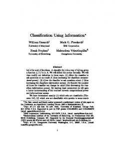
2.3. Normalizing maps and transition functions. Now we apply these statements to SN-families in preliminary normal form. Let F be such a family. Denote by v the associated family of vector elds dened by (2.2). From the hyperbolicity of xed points of both F and its formal normal form F~ = gv1 and the coincidence of the corresponding multiplicators in the domain " > 0 , it follows that F and F~ are smoothly conjugated in a certain neighborhood S+ of the positive branch ;+ = fx = +p" " > 0g of the parabola ; : there exists a transformation H+ dened on S+ of the form (x ") 7! (H+ (x ") ") such that H+ F = F~ H+ in S+ \ F;1 (S+ ) . p Since the xed point p x = + " is unstable, its basin of repulsion includes the interval (;p" ") between the xed points. By the Corollary to Lemma 2, the map H( ") can be uniquely extended to this interval. In a similar way the map H; = (H; id) can be dened in a certain neighborhood S; of the set ;; = fx = ;p" " > 0g and then extended to the domain D = f" > 0 jx2j < "g .


17

Fig. 1. Basins of attraction and repulsion. Thus we obtain two maps H , both dened on D and conjugating the given family F with its formal normal form F~ . Their ratio = H+ H;;1 : D ! D = ((x ") ") (2.3) is a smooth map dened in the (open) domain D which commutes with F~ . If H~ denote any other pair of smooth maps conjugating F with its formal normal form in the domains S , then by Lemma 2 they must dier only by the ow map of the standard eld: there exist two functions (") smooth on a certain interval 0 < " < "0 such that H~ (x ") = H gv (("")) x " : The ratio ~ = H~ + H~ ;;1 is related to as ~ = gv+ gv;;

(2.4)

where gv stand for the ow maps (x ") 7! gv(("")) x " . Since the normalizing charts are invariantly associated with SN-families, the transition function is also invariant by at least C 1-smooth transformations up to the equivalence (2.4). Note that the equivalence relation (2.4) explicitly depends on " . In order to avoid such an inconvenience, let us introduce a new chart t straightening the family v . Dene the family of maps t : (R1 0) (R1+ 0) ! R1 (R1+ 0) t = (t id) where x ; p" 1 1 t = t(x ") = 2p" ln x + p" + 2 a(") ln jx2 ; "j " > 0 (2.5)

18


Note that this family of maps depends explicitly on the choice of the germ a(") : from now on we assume that condition (2.1) is satised. The map (x ") 7! t(x) transforms the eld v = (x2 ; ")(1 + a(")x);1 @=@x into the constant eld @=@t in the coordinate t , the family F~ becomes the unit shift id +1 . Therefore the transition map (when written in this coordinate) commutes with the unit shift: if we denote (' id) = t t;1 , then the preservation of the second coordinate implies that '(t + 1) = '(t) + 1: (2.6) The dierence ' ; id = is a 1-periodic function: (t + 1) = (t) . If ~ are two families of maps equivalent in the sense of (2.4), then the corresponding functions ~ dier by a shift in the source space: ~ ") = (t + (") "): (t (2.7) This form is similar to the one used in x2 of paper I. 2.4. The moduli space. The above construction motivates the following denitions modeled after the patterns given in Paper I. Consider the Cartesian product M = R2+ P where the half-plane R2+ is endowed with the coordinates " > 0 a 2 R1 and P denotes the space of smooth 1-periodic functions on the real line. ~ 2 M are said to be Definition. Two elements (" a ) (~" a~ ) equivalent, if (" a) = (~" ~a) and there exists a 2 R such that = ~ (id+) . Denote the space of all equivalence classes by M . The above construction permits to associate to every saddle-node family F in preliminary normal form a parameterized curve in the moduli space: = F : (R1+ 0) ! M " 7! (" a(") (t ")) (2.8) This curve is smooth for " > 0 : this means that a(") is the smooth germ and the last component (( ")) is a smooth family of 1-periodic functions. We will use the notion of a smooth parameterized curve also in the quotient space M , meaning that there exists a smooth curve consisting of representatives of equivalence classes. In the terminology introduced above, the results obtained in 2.2, 2.3 can be formulated in a geometric way. Proposition. Two saddle-node families F1 and F2 in preliminary normal form are conjugated only if the corresponding parameterized curves 1 , 2 : (R1+ 0) ! M in the space of moduli are pointwise equivalent:

8" > 0 1 (") 2("):


19

To transform this proposition into a full-scale classication theorem, one needs to investigate possible types of parameterized curves which can be realized as invariants of SN-families. This investigation is based on a detailed description of the normalizing charts H , provided by the sectorial normalization theorem formulated in the next section.

x3. Embedding in a ow: the key to the classi cation of saddle-node families Consider a smooth SN-family F in preliminary normal form along with

the associated family v of vector elds. We construct a conjugacy between the family F and its formal normal form F~ = gv1 in domains of a special form. ; 3.1. Embedding in sectors. Let + R2 0 be the closed domain of the form f; 2 6 " 6 0 jxj 6 g f0 6 " 6 2 > x > ;2"g and ; its mirror image in the "-axis. Here is a small positive parameter to be chosen afterwards. Sectorial embedding theorem for SN-families. For all suciently small > 0 in each domain there exist maps H smooth in the sense of Denition 4, x0,

H : (x ") 7! (H(x ") ")

possessing the following properties: (1) each H preserves the parameter and conjugates F and its formal normal form F~ (2) for " 6 0 the two maps identically coincide: H+ ( ") H; ( ") (3) in the connected component jxj 6 2" of the intersection + \ ; belonging to the positive half-plane f" > 0g , the two maps dier by a function which is at at the origin:

H+ H;;1 = (id +'(x ") id)

where '(x ") along with all its derivatives decreases more rapidly than any power of " as " ! 0+ jxj 6 2" . Remark. The possibility of representing an individual nonhyperbolic mapping F( 0) as the time 1 map for a vector eld on the line was proved by F. Takens T2]. This Takens generator is uniquely determined. On the other hand, by the Corollary to Lemma 2, each hyperbolic singularity x = p" uniquely denes the \hyperbolic" generator in the open quadrants f" >

20


0 x > 0g . The sectorial embedding theorem means that the \hyperbolic generators" can be smoothly extended on the x-axis by the above Takens generator. Finally note that for " < 0 there are no xed points at all, so the existence of the generator becomes a trivial statement, while uniqueness no longer holds. The rst assertion of the theorem implies that the smooth continuations of the \hyperbolic generators" across both positive and negative semiaxes can be chosen to coincide with each other in the negative half-plane. The proof of the theorem is rather technical, although transparent: it is postponed till the second part of the paper. Now we turn to applications.

3.2. Classi cation of saddle-node families. Let F1 F2 be two SNfamilies already in their preliminary normal forms. Then the coincidence of the corresponding formal normal forms (i.e. the identity a1 (") a2 (") for " > 0 ) is a necessary condition for their equivalence. One can dene the corresponding normalizing charts H i i = 1 2 , and the transition functions i = (i id) . This necessary condition being satised, the equivalence relation (2.4) makes sense for " > 0 , since the eld v is the same for both families. Now we can formulate the following main result. Classification theorem for SN-families. Two local SN-families in preliminary normal form are smoothly conjugate if and only if they are formally equivalent (i.e. they have the same formal normal form), and their functional invariants i are equivalent in the sense of (2.4). Moreover, any pair (F~ ) consisting of a standard family (the formal normal form) and family of functions dened on + \ ; and commuting with F~ can be realized in an appropriate SN-family as the invariant of smooth classication, provided that diers from identity by a function at at the origin. Remark. The necessity part of the theorem is evident as explained above.

Note also that we do not require the coincidence of the formal parts for " < 0 , because Corollary 2 to the Theorem in x1 implies that two C 1 -smooth families of elds coinciding for positive " are automatically C 1 -equivalent. Proof. Applying the sectorial embedding theorem, one may assume that the entire neighborhood of the origin in the (x ")-plane is covered by two charts i i = 1 2 with local coordinates (xi ") , xi = H i (x ") such that in each chart the corresponding family Fi is precisely the time 1 map for the same vector eld v . Moreover, since the transition functions for the two families dier only by a ow map, one can choose another pair of normalizing charts, say, for F1 , so that the transition functions will coincide


21

identically on their domains: 1( ") 2 ( ") for " > 0 . Dene the conjugacy H between the families as the map which is identical in the charts of the same \sign" so that the following diagram is commutative: R2

+ 1 ; 1 H;;;; + 1 ; 1 ;H;;;!

R2

R2

+ 2 ; 2 H;;;; + 2 ; 2 ;H;;;!

R2

? id? y

? H? y

?? yid

Since all the charts are smooth and the denition of H on the intersection of domains is self-consistent, the above diagram provides the desired equivalence. Let us proceed with the proof of the realization part of the Theorem. We follow the standard pattern suggested in Paper I. Without loss of generality we may assume that the formal normal form of the family to be realized is the standard one: F~ = gv1 v = (x2 ; ")(1 + a(")x);1 @=@x . Consider the disjoint union of two open sets int belonging to two distinct copies of the real plane R2 with the coordinates (x " ) . Dene the smooth maps F on these sets as the standard family F~ written in these coordinates, see (2.2). Let = ((x ") id) be the given map which is to be realized as the modulus of the classication. By the assumptions, maps the sector fjxj < 2" 0 < " < "0 g into a nearby curvilinear one with the same vertex, preserves the "-coordinate and commutes with the restriction of F~ on the sector. Moreover, this map is 1-tangent to the identity at the origin. Dene the quotient space of the union + ; using as the identifying map. More precisely, we identify two points (x " ) 2 int if "+ = "; (this common parameter value will be denoted by " ), and one of the following holds: either " < 0 , and x+ = x; , or " > 0 , and x+ = (x; ") . As usual, we may consider the sets int as charts on with extended by the identity to the negative half-plane as the transition function for the corresponding atlas. The quotient space is homeomorphic to a punctured neighborhood of the origin on the plane. We show that can be completed by a point in such a way that the completion ~ retains the structure of a smooth manifold. Indeed, dene the map H : ! R2 in the coordinates (x " ) by the formula

H(x ") = (+ x+ + ;x; ") where f g is a smooth partition of unity subjected to the covering int with polynomial growth of derivatives H]. The polynomial growth condition means that all the derivatives of the truncating functions can be estimated

22


by certain powers j"j;l jxj;d in the sectors as (x ") ! (0 0) , the exponents depending on the order of the derivative. On the intersection of charts, this map admits the following representation: + x+ + ; x; = + (x; ") + ; x; = x; + + '(x; ") (z) (for simplicity we put ' equal zero for negative values of " ). The map H denes the embedding of in R2 . We endow with the smooth structure inherited from the plane. Adding the point corresponding to the origin in the plane to ensures that the result ~ is dieomorphic to an entire neighborhood of the origin. Denote this neighborhood by U . Now we dene the saddle-node family in U . To do this, recall that there are two maps F in the charts int . Since the identifying map used in the construction of the quotient space commutes with them ( F+ = F; ), we can consider the unied map F : ! . We pull it back into U n f0g , using the chart H , by setting F = H F H;1 . Obviously, the map F is smooth outside the origin. Now our problem is to extend F to the origin while preserving its smoothness. Set F(0) = 0 . One needs only to prove that this extension is smooth at the origin. From (z) it follows that the chart H diers from either x+ or x; by functions at at the origin, while the map F is given in both charts x by the same formula. Hence all derivatives of F with respect to the chart H have the same limits at the origin as those of F with respect to x . Since the latter functions are smooth, the conditions of the Whitney continuation theorem H] hold for them. These same conditions also hold for F at the origin by continuity. This ensures the possibility of smooth extension. This extension is unique for obvious reasons: limx "!0 F(x ") = 0 . So we have constructed a smooth local family of line dieomorphisms. Let us verify that the family F is indeed of the SN-type. To prove this, note that this family for " > 0 has two hyperbolic xed points with the same multiplicators as in the family F~ = gv1 . The smoothness of H at zero (see item (3) of the sectorial normalization theorem for SN-families) implies that the xed points of the map F ( 0) have multiplicity 2. Therefore the preliminary normal form condition is satised and the formal normal form is as required. The functional invariant for F is equal to , since the x H;1 form the normalizing atlas with that same transition function. The realization part is proven. The sectorial normalization theorem has a geometric corollary for parameterized curves (in the function space) associated with smooth SN-families. These curves are smooth not only on the interior of the interval 0 < " < "0 , but also at the left boundary point " = 0 . This means that the family (t ")


23

of functional invariants constructed in the preceding section possesses certain limits for all its derivatives either in t or in " as " ! 0+ . Moreover, the function (t ") tends to zero together with all its derivatives as " ! 0+ . Indeed, a similar property holds for the dierences ' = ; id as asserted in the theorem. The rest follows from the polynomial growth of the straightening chart t given by (2.5).

x4. Applications to bifurcation theory.

In order to give an example of the application of the sectorial embedding theorem, let us prove the suciency of the Malta{Palis conditions MP] describing the simultaneous occurrence of multiple saddle connections in a generic two-parameter family of planar vector elds. 4.1. Semistable cycles and multiple saddle connections. Consider a planar vector eld having a semistable limit cycle with a monodromy transformation ; ; %: R1 0 ! R1 0 %(x) = x + ax2 + O(x3) a 6= 0 such that there are at least two topologically distinct trajectories tending to the cycle from the inside as well as from the outside (for example, these trajectories may be stable and unstable separatrices of hyperbolic saddles, see Fig. 2).

Fig. 2. Semistable limit cycle with topologically distinct curves from both sides. In a generic deformation of the eld such a cycle disappears and one or more saddle connections (i.e. heteroclinic orbits of the eld) may occur. Let us examine whether the simultaneous occurrence of several saddle connections is possible or not. Proceeding in the standard way, we reduce the problem

24


to the investigation of orbits of the monodromy maps. These maps form a saddle-node family of line dieomorphisms x 7! F (x ") . The topologically distinguished trajectories intersect the transversal to the cycle on which the monodromy is dened. This intersection for " = 0 consists of semi-innite orbits of F (either positive orbits for the trajectories converging to the cycle or negative ones corresponding to the trajectories converging to the cycle after time reversal). We consider the case where there are at least two orbits from each side. Take a unique representative from each orbit in its intersection with the transversal. Denote them by xi , where xi+ i = 1 2 is the pair of points belonging to the trajectories converging to the cycle with time increasing, while xi; i = 1 2 stand for the other pair of orbits. Without loss of generality we may assume that x1+ < x2+ < 0 < x1; < x2; . Note that, by transversality, all the xi smoothly depend on the parameter. We are interested in conditions guaranteeing that no pair of these points belongs to the same orbit of F for " < 0 . These conditions were found in MP]. In order to formulate them, recall that the individual monodromy map %( 0) can be embedded in a ow v by the Takens theorem. Dene the two numbers by the following conditions: gv x1 = x2 (4.1) The values measure the distance between the orbits coming from the same side, in units of time. So they make sense only mod Z. Theorem MP]. If we have + 6= ; mod Z (4.2) then the simultaneous occurrence of two saddle connections is impossible.

We shall prove that this necessary condition is actually very close to the sucient one. Theorem on multiple saddle connections. If condition (4:2) is vi-

olated in a generic two-parameter family of planar vector elds, then there are countably many values of the parameters (accumulating to the critical value) for which two saddle connections occur simultaneously. Proof. Without loss of generality one may assume that the violation of (4.1) implies + = ; (otherwise another representative from the orbit must be chosen). Let (" ) be the two parameters, so that the monodromy map takes the form % = F ( " ) . It follows from the transversality theorem that values of parameters for which the map F has a double xed point


25

belong to a smooth curve & passing through the origin on the parameter plane.

Fig. 3. Bifurcation diagram on the parameter plane. One may assume that this curve is f" = 0g and that for " < 0 there are no xed points at all. Apply the sectorial embedding theorem to the family F . This theorem provides a smooth family of vector elds v = v(x " ) @=@x dened for negative " and such that F is the time 1 map for v . So one may dene instead of two numbers , two germs of functions (" ) " < 0 by the following conditions: (" ) =

x2Z(" ) x1 (" )

dx v(x " ) :

(4.3)

Since the eld v is nowhere vanishing on the segment of integration, these functions are smooth. For a generic family of maps the curve ; = f(" ) 2 R2 : + (" ) = ; (" )g is smooth and transversal to & . Note that a saddle connection between the points x1+ and x1; occurs if and only if T1 (" ) =

x1;Z(" )

x1+ (" )

dx = n 2 N v(x " )

(4.4)

(a similar condition for the other pair has the form T2 2 N ). The corresponding curves &n = f" : T1 (" ) = ng in the parameter plane are

26


accumulating to & as n ! 1 , see Fig. 2. This follows from the fact that the integral (4.4) uniformely tends to innity as " ! 0 . Now note the following obvious fact: on the curve ; one has + = ; , therefore each point of the intersection &n \ ; corresponds to the occurence of a double saddle connection. This intersection contains countably many points accumulating to the origin and lying on the smooth curve ; .

4.2. Asymptotics of the trapping time. Another application of the sectorial embedding theorem is the computation of the asymptotics of trapping time. Consider a planar analytic vector family of vector elds having a semistable limit cycle for a critical value of the parameters and suppose that by small perturbations of parameters this cycle is pushed away from the real into the complex domain. Nevertheless all trajectories for the perturbed system remain trapped near the place where the cycle was for a suciently long time. This time was estimated in DV] in terms of the imaginary parts of the multiplicators of the (complex) xed points of the monodromy. The analyticity is irrelevant, since the sectorial embedding theorem implies the following estimate of the trapping time for smooth families. Suppose that a smooth generic one-parameter family of planar vector elds depending on a real parameter " possesses a semistable limit cycle C0 for " = 0 , which splits into two hyperbolic cycles C (") when " becomes positive. Take any transversal to the semistable cycle. Then these two hyperbolic cycles intersect at two points between which the distance is d(") p" . For any suciently narrow annulus-like open domain U containing C0 and any suciently small negative " denote by N = N(U ") the number of full turns made by a trajectory conned within U . We are going to estimate the principal term of the asymptotics of N(U ") . The trapping time estimate. For any U

N(U ") = 2d(j"j) + O(1)

" < 0 " ! 0; :

(4.5)

Proof. First we point out that the number N is dened in terms of

orbits rather than of the eld itself: multiplication of the eld by a positive nonvanishing function changes the trapping time and the \period" of one rotation, preserving the number N . Moreover, we can replace the domain U by the ow box U0 bounded by two segments of integral curves between subsequent intersections with and segments of the transversal itself: this will change the number N by a bounded term. Let % = % ( ") be the monodromy map. Then the trapping \time" is


equal to

n

27

o

n] N(U0 ") = inf n n: % (; ") > + where is a small positive number (corresponding to the boundary of the ow box U0 ). Let us embed the family of monodromy maps in the smooth ow. Then the trapping time is equal to the integral dening the time necessary to get from the outer boundary of the annulus to the inner one. This integral can be explicitly computed provided that the ow is standard, and the principal term of its asymptotics equals Z + dx = p N(U0 "~) 2 x ; " ~ j"~j ; where "~ is the parameter occurring in the preliminary normal form this parameter is p expressed via the distance d between the singular points of the generator as ;"~ = d(;"~) , whence the specic form of the formula (4.5). Evidently this result can be generalized for the multidimensional case.

x5. Sectorial normalization and smooth classi cation of ip families.

In this section we show that in domains of a certain special form a ip family is conjugated with the superposition of the time 1/2 map for an odd family of vector elds and with the standard symmetry x 7! ;x preserving this family. 5.1. Iteration square of ip families: embedding in a ow. Let F = (F id) be a ip family in the preliminary normal form. As it was shown in 1.2, this family has the form F (x ") = ;x + x(x2 ; ")f(x ") (5.1) with a smooth function f such that f(0 0) = 1 . The iteration square F2] is the family which is a transversal deformation of the line dieomorphism tangent to the identity with the third order at the origin: (5.2) F2] = (F2 id) F2(x ") = x + x(x2 ; ")f2 (x "): The specic trait of the case (5.2) is that F2 ( 0) has a triple xed point at the origin instead of a double. The representation (5.2) implies that the xed points of F2] lie on the \trident" fx(x2 ; ") = 0g . Nevertheless, all the xed points of F2 for " 6= 0 are hyperbolic. This circumstance allows to modify the construction developed in x3 in order to obtain the smooth classication of ip families.

28


Let + ; be two closed domains in the (x ")-plane: ; = f; 2 6 " 6 0 jxj 6 g f0 6 " 6 2 jxj > "g (5.3) + = f0 6 " 6 2 jxj 6 4"g: The intersection + \; consists of two sectors f0 6 " 6 2 " 6 x 6 4"g , each of which is wide enough to include some fundamental domain of the action of F2 in the positive half-plane " > 0 . Consider a smooth family of vector elds of the form @ +0 @ (5.4) w(x ") = x(x2 ; ")(1 + b(")x2 ) @x @" where the smooth function b = b(") is chosen in such a way that gw1 has the same multiplicators of all xed points as the family F2] . Sectorial normalization theorem for \trident" families. For all suciently small values of > 0 , in each domain there exist smooth maps H = (H id) which conjugate F2] and gw1 these maps dier on the intersection + \ ; by a function which is at at the origin:

;1

H+ H; = (id +' id)+ ' = '(x ") \ : Dx D" '(x ") ! 0 as x ! 0 (x ") 2 + ;

We do not give the proof of this theorem, since it reproduces essentially that of the analogous theorem for saddle-node families. Let us turn directly to implications.

5.2. Involutions and ows. We had just asserted the possibility of embedding orientation-preserving families which are the squares of ip-type ones in a ow. Since a true ip is orientation-reversing, it cannot be represented as the time 1 map for any ow. Nevertheless we can split a ip family into the superposition of the standard involution and a ow map. Consider two elds w = (H ) ;1 w on . Both of them are generators for the family F2] on the corresponding domains, therefore they are preserved by F2] : F2] (5.5) w = w : Our immediate goal is to prove that the initial orientation-reversing ip family F also satises this property. Proposition. Both elds w are preserved by F : Fw = w: (5.6)


29

F commutes with the time t maps gwt for all t 2 R . Proof. Consider the elds w~ = F w on . Let us prove that they also are generators for the family F2] . In this case the hyperbolicity of xed points of F2] j" , where " = const = 6 0 , implies that w~ = w , since the Corollary.

generator is unique. Indeed, F2] preserves w~ : from the commutation of powers of F and property (5.5), it follows that F2] w~ = (F2] F) w = (F F2] ) w = F w = w~ : Now note that any eld preserved by F2] ( ") " 6= 0 , diers from the generator of F2] by a scalar factor, so w~ = (")w . Computation of 1-jets at the xed points yields (") 1 for " 6= 0 . From continuity arguments it follows that w~ w . Dene the pair of maps = F gw;1=2: These maps are involutions: this follows from the previous corollary and the denition of w . Moreover, these involutions preserve the corresponding elds: ( ) w = w . Lemma. In both domains there exists a smooth map H which takes the corresponding eld w to polynomial form (5:4) and at the same time transforms into the standard symmetry x 7! ;x . Proof. We demonstrate the statements in several steps. For the sake of simplicity the subscripts referring to the choice of the domain will be omitted. 1. Polynomial normal form. There exists a smooth transformation taking the family w to polynomial normal form (see Corollary 1 to the Theorem in x1). This polynomial is of degree 5 since the zeros of the eld lie on the \trident" fx(x2 ; ") = 0g , one may assume that the eld is of the form @ w = x(x2 ; ")(b0 + b1x + b2x2) @x (5.7) where bi = bi (") stand for smooth germs. 2. Oddity. Let us show that an odd polynomial in (5.7) may in fact be chosen. This step is implemented somewhat dierently for + and ; . If the case ; is considered, then one can note that the eigenvalues of w corresponding to the zeros @w=@x(p" ") , coincide, since there is the automorphism of the eld which swaps these zeros. So for " > 0 we have b1(") 0 . The T heorem of x1 implies that one may put b1 identically equal to zero: indeed, the function b1(")x2 (x2 ; ") is divisible by x2 (x2 ; ")2 in ; provided that b1 is as above.

30


In the case of + the situation is even simpler, since b1x2 (x2 ; ") is divisible by the same factor in + . 3. The involution. It remains only to prove that any orientation-reversing automorphism preserving the odd family w = x(x2 ; ")(1 + b(")x2 ) @=@x = xk(x2 ") @=@x (5.8) must be the standard symmetry. Indeed, if we write : (x ") 7! (s(x ") ") , then the graph y = s(x ") must be an integral curve of the following system on the (x y)-plane: dy = yk(y2 ") (5.9) dx xk(x2 ")

(see (5.8)). Note that for " 6= 0 the singular point (0 0) of (5.9) is the dicritical node : they became nonsingular after blowing up AI]. So we have uniqueness of smooth continuation of integral curves through dicritical nodes: for any direction there is a unique pair of integral curves of the system in a neighborhood of a dicritical node which becomes a smooth curve tangent to the given direction after adding the singular point. If we choose the antidiagonal direction, then the curve y = ;x is the integral one for (5.9) in the case " 6= 0 , hence it must coincide with the graph of s . In the case: " = 0 , we have the same assertion: s = fy = ;xg is true by continuity. So we have proved the last assertion of the lemma.

5.3. The \sectorial embedding" in the ip case. Let F = (F id) be a ip family in preliminary normal form (1.6) denote by F0 = (F0 id) the local ip family F0 = gw1=2 where w = wF is the smooth odd family (5.8) constructed using the corollary to Lemma 1B, x1, and is the standard symmetry in the "-axis. Sectorial normalization theorem for the flip case. If the parameter determining the size of the domains is suciently small, then there exists a pair of maps H = (H id) , dened and smooth on these domains, such that: (1) in each domain the corresponding map conjugates the restriction Fj with the normal form F0j :

H F0j = FjH ( ) H (2) any other pair H~ of maps satisfying the above property must dier from H by a ow transformation in the target space: there exists


31

a pair of smooth germs = (") such that

H~ = gw H

where

gw (x ") = (gw (("")) x ")

(x ") 2

(3) the maps H normalizing the family F may be chosen so as to

have a common 1-jet at the origin: in other words, their iteration ratio = H+ H;;1 = (id +'(x ") id) diers from the identity by a function ' dened in the union of two sectors with the common vertex at the origin, and at at this vertex.

Proof. The existence of the normalizing charts follows immediately from the above lemma. The third assertion holds, since the embedding theorem for \trident" families asserts an analogous property. It only remains to prove the second assertion which is a kind of uniqueness. Note that any other normalizing charts must preserve the local generators w due to the hyperbolicity of the xed points of F2] . Hence the normalizing charts must dier by a ow map as it was shown in x2. A minor diculty arises from the fact that the intersection ; \ f" = const > 0g is not connected, so a priori two dierent values of the shift time, each for its own connected component of the intersection are possible. In fact, nothing of that kind occurs. Indeed, the iteration ratio of the normalizing charts commutes not only with F2] , but also with F : this implies that must commute with the standard involution, thus being odd. If we try to nd an odd map of the form gw1 (") gw;2 (") dened on + \ ; , we necessarily come to the conclusion that 1 2 . The classication theorem for ip families follows from the sectorial normalization theorem precisely as it was in the SN-case. We can introduce a straightening chart t and dene an analogous notion of equivalence on the set of transition functions written in this chart. Note the following fact. Since the intersection + \ ; consists of two sectors, one may expect that the invariant consists of two transition functions. This is not so, since the equivalence of transition functions, say, in the upper sector of the intersection, implies automatically the equivalence of those corresponding to the lower one: indeed, the family F swaps these sectors. In order to get rid of repetitions, we omit the realization statement (which is true for sure) and formulate the classication theorem for ip families in the following way.

32


Classification theorem for flip families. Two ip families F1 F2 in preliminary normal form are conjugate if and only if the corresponding 2] \trident" families F2] 1 F2 are conjugate.

Clearly, this is simply a reformulation of the equivalence of the transition functions.

x6. Smooth orbital classi cation of Andronov{Hopf families. 6.1. Semimonodromy. Let V = V (z ") @=@z z 2 (C 0) ' ;R2 0

be a smooth local AH-family. As we mentioned in the Introduction, it takes the form V(z ") = zA(z ") @z@ (6.1) @Re A Re A(0 0) = 0 ImA(0 0) = ! > 0 @" (0 0) 6= 0 with a smooth complex-valued function A in; a certain complex coordinate system on the plane. Note that for each " 2 R1 0 the eld V( ") has a unique singularity at the origin which is hyperbolic for " 6= 0 . Our study of AH-families is based on the investigation of the rst return map dened as follows. Let be a germ of a smooth curve passing through the singularity and tangent to a certain direction. Note that the polar angle function Arg z on the complex plane C monotonically increases along orbits of the family (6.1), at least in a suciently small neighborhood of the singularity. So for any point b 2 close enough to the origin the positive semitrajectory gVt b t > 0 , intersects at least once. Definition. A semimonodromy map (or, more precisely, a local family of maps) for a family V , dened on a smooth curve , is the map taking a point b 2 b 6= 0 to the rst intersection of the positive semiorbit starting at b with . We shall denote the semimonodromy map by % . An analogous construction is well-known for the case when there is a periodic orbit ; of the eld V and is a smooth curve transversal to ; . In this case the general theorems on dierentiable dependence of solutions of ODE's on initial conditions imply the dierentiability of the corresponding rst return map. In our situation these results cannot be applied, since there is no transversality at the singular point. For a generic singularity, the rst return map, even if dened, is not smooth. Nevertheless, the AH-case proves to be an exception.


33

Proposition. If V is an AH-family in the form (6.1), then for any smooth curve passing through the origin, the semimonodromy % is a smooth local family of orientation-reversing maps depending smoothly on the parameter. If 1 is another smooth curve, then the corresponding semimonodromy %1 is conjugate with % .

Proof. This assertion becomes evident after passing to polar coordinates on the plane. ; More precisely, let C be a cylinder with coordinates r 2 R1 0 ' 2 S 1 ' R=2Z. Dene the map ( : C ! C ((r ') = r exp i' (the inverse (;1 is given by r = jz j ' = Arg z mod 2 ). The inverse image V~ = (; 1 V of the eld V is smooth on C and admits a unique smooth continuation on the circle ; = fr = 0g . Indeed, one can write the equation corresponding to the eld V in the form A(z ") = zz_ = (Ln z)_= (ln jz j + i Arg z)_ = rr_ + i'_ whence r_ = r Re A(r exp i' ") '_ = ImA(r exp i' "): Since ImA(0 0) 6= 0 , it is clear from these formula that ; is an invariant curve for V~ . Now note that the inverse image (;1 () consists of two smooth curves and of the circle ; , and the covering transformation T : (r ') 7! (;r ' + ) maps one onto the other dieomorphically. Moreover, the restriction ( = (j maps dieomorphically onto . Finally note that the map % : + ! ; taking each point to the rst intersection of the corresponding positive semiorbit of V~ with the other curve, is smooth, since both are transversal to V~ . All these facts imply that the semimonodromy % , which can be expressed as the superposition (+ % (;;1 = (; T % (;;1 , is a smooth map. The second assertion is no less evident, since for another choice of the curve 1 one has another pair of smooth curves 1 on C , and the desired smooth conjugation is realized in the polar coordinates by a map + ! 1 + dened again as the rst intersection correspondence. Remark. Computation of higher order terms shows that the semimonodromy map associated with an AH-family is indeed of SN-type.

6.2. Semimonodromy and orbital equivalence. If there are two AH-families V1 V2 , and % i = 1 2 , are their semimonodromies corresponding to the curves i , then orbital equivalence between Vi implies smooth equivalence of the germs % . Indeed, multiplication of a eld by a positive function does not change its semimonodromy. On the other hand, if i

i

34


H is a map conjugating the ows of Vi , then its restriction to 1 conjugates

the semimonodromies %1 and %H(1 ) , the latter one being conjugated with %2 by the above proposition. We are interested in the inverse statement. Classification theorem for Andronov{Hopf families. Two AHfamilies are orbitally equivalent if and only if the corresponding monodromies, being ip-type local families, are smoothly conjugate. Any ip family can be realized as the semimonodromy map for an appropriate AH-family.

The rest of the section is devoted to the proof of this statement. An idea is evident. If there are two AH-families zAi (z ") @=@z , then one can divide these families by appropriate real functions so that Im Ai 2 . Choose the germ of the positive semiaxis as a semitransversal i in both cases. Then the semimonodromies associated with this choice are simply the time 1/2 maps gi1=2 for the corresponding ows fgit g , i = 1 2 . Suppose that these semimonodromies are smoothly conjugate, i.e. there exists a smooth real family h of maps dened on the real line and conjugating gi1=2 . Extend h to an entire neighborhood of the origin (C 0) by the formula H(z ") = g2 2 h g1; Arg z

Arg z 2 z

z 6= 0

H(0 ") = 0:

(6.2)

The relation (6.2) is correct, since for any point z one has Arg g1; =0 by the above convention imposed on the functions Ai . The map H in fact is not multivalued, though the function Arg is: if we choose another value of Arg , diering by 2k k 2 Z from the initial one, then the whole expression will not be changed. This is a consequence of the identity g21 h = h g11 that follows from the above conjugacy. The only problem is to prove smoothness of H at the origin. To do this, one needs a certain special coordinate system in which the given AH-family will be almost rotationally symmetrical. Arg z 2 z

6.3. Preliminary normal form for the Andronov{Hopf case. Lemma. Any local AH-family V is orbitally equivalent to a family V0 of

the form where:

V0(z ") = z (R(z ") + 2i + F (z ")) @z@

(1) both functions R F are real and smooth

(6.3)


35

(2) R is rotationally ; symmetrical, ; i.e. R(z ; ") = (zz ") with some smooth real : R1 0 R1 0 ! R1 0 (3) F is at at the origin z = 0 for all " . We shall refer to the eld z(R + 2i) @=@z as the symmetrical part of V0 , while F @=@z will be called the at perturbation. Proof. Let us associate with each smooth local family V its semiformal Taylor series

X

@ ak l (")z k z l @z k l>0 with ak l being smooth functions dened in some neighborhood of zero, common for all k l , in the parameter space. On the set of such semiformal vector elds a natural action of the group of semiformal transformations of the form

X k l (z ") 7! z + hk l (")z z "

V^ = z

k l>0 k+l>2

is dened. Normal forms in the semiformal category are very close to those of Poincar+e{Dulac (see A] ). For example, using semiformal transformations, one can put the series V^ corresponding to the initial AH-family into the form

^V1 = z X ak k (")(zz)k @ (6.4) @z k>0

containing only terms corresponding to the resonance + = 0 , which takes place for " = 0 . Consider the semiformal transformation putting the initial series into the form (6.4) and extend it to a smooth family of plane transformations with the same Taylor series, using the Borel{Whitney continuation theorem. After applying this extension to the family V , one obtains a smooth family of planar vector elds having (6.4) as its semiformal Tailor series. This means that the new family acquires the desired form after division by an appropriate real positive smooth function. For a more detailed exposition of the semiformal techniques see IY]. 6.4. Proof of the suciency assertion. Consider a family V in the form (6.3) and choose the positive semiaxis as the semitransversal . Then the semimonodromy associated with such choice equals % = ;gw1=2 + (at function) (6.5) where w = x(x2 ") @=@x is an odd family of vector elds on the real line. For the family w the origin is an isolated singularity, hyperbolic for " 6= 0 .

36


Suppose that there is a smooth family h = h(x ") conjugating two maps %1 %2 , both of the form (6.5) with dierent vector elds w : w1 and w2 respectively. The above mentioned hyperbolicity implies, that: (1) the function h is almost odd in the given coordinate: h(x ") + h(;x ") = (at function) (2) h almost conjugates the corresponding elds: h w1 ; w2 = vector eld, at at the origin for all ": The proof of both statements deals with formal Taylor series. It is almost evident when " 6= 0 and the elds w ; 1 , w2 are equivalent to linear ones near the singular point x = 0 . The case " = 0 comes by continuity. Let V1 V2 be two families in the form (6.3) with semimonodromies as above, conjugated by a smooth map h = (h id) . Consider the antisymmetrisation h~ (x ") = (1=2) (h(x ") ; h(;x ")) , which diers from h by a at function. This antisymmetrisation can be extended to a plane transformation ~ ") = (z=jz j)~h(jz j ") . Since ~h is odd, H~ is smooth. After applying H~ H(z to the rst family V1 we obtain another family (denoted again by the same symbol), so that: (1) V1 is again in the form (6.3) (2) its symmetrical part coincides with that of V2 up to a at symmetrical eld (3) there exists a conjugation (denoted again by h ) between semimonodromies of Vi , which diers from the identity by a at function. This list of properties implies the smoothness of the map H dened by (6.2). Indeed, one can easily check that all maps in the superposition have the form id+(at function) . For h this is explicitly asserted above. The ow maps git for elds Vi dier by a at function uniformly in t , since their 1-jets at the origin coincide. Finally, the polar angle function Arg z along with all its derivatives has no more than polynomial growth in jz j;1 as jz j ! 0 . So the whole superposition diers from the identity by a at function, thus being smooth at the origin. 6.5. Realization. Consider a ip family F . Let us prove that there exists an AH-family of vector elds on the plane which has the semimonodromy conjugated to F . To do that, we shall use the sectorial inclusion theorem for ip families established in x5. Let + ; be the standard domains in which the given ip family has the form @ (x ") = (;x ") (6.6) F = gw1=2 w = x(x2 ; ")(1 + b(")x2) @x


37

and denote by the odd transition ;function between the normalizing charts. Dene two domains S in C R1 0 as the sets of (z ") such that (jz j ") belongs to . In each domain S consider the symmetrical family of vector elds V = z 2i + (zz ; ")(1 + b(")zz)] @z@ z 2 S : If we choose the axis as the semitransversal , then the semimonodromy of V (where it is dened), has the standard form (6.6). Denote the ow maps of these elds by gt respectively. Now consider the intersection S+ \ S; . This intersection is the region between two straight cones centered around the positive semiaxis. In each plane " = const > 0 it is seen as the annulus f" < jz j < 4"g . The transition function restricted to the plane " = const can be identied with a map of the intersection of this ring onto a nearby one, odd and commuting with the time 1 map for the ow of the eld w . Dene the map H of the intersection S+ \ S; into a nearby one by the formula Arg Arg H(z ") = g;2 g+; 2 z: One can see that H is well-dened because and g1=2 commute. Moreover, since diers from the identity by a function at at the origin, the same is true for H . Using H as the identifying map, one obtains from the disjoint union S+ S; an abstract 3-dimensional manifold with a foliation originating from " = const and with a vector eld tangent to this foliation. The general argument described at least twice (in 3.2 above and in Paper I) is now applicable: we endow the quotient space with a smooth structure using a partition of unity and then show that the eld obtained is indeed of the type required. By construction, this eld has the given family F as the semimonodromy. The proof of the classication theorem for Andronov{Hopf families is complete.

z

z

Part II. Proof of the sectorial embedding theorem.

x7. Jets and operations on them.

From now on our exposition will be entirely devoted to the proof of the sectorial embedding theorem, see 3.1. The embedding is implemented in two steps. In both steps our main tools will be jets and at functions, dened below. A jet is, roughly speaking, a collection of derivatives with prescribed values on a given xed subset K Rn .

38


The rst step is to solve the embedding problem in jets on an appropriate set. After this task being completed, we obtain a smooth eld whose time 1 map coincides with the given SN-family up to a correction which is at on K . This means that all derivatives of the correction are rapidly decreasing if their argument tends to K . The second step is to show that two SN-families diering by a at correction are smoothly conjugate. In fact this is not true, but the conjugation exists in the sector-like domains introduced above. The main reason that this step can be carried out is that the set K contains not only xed points of F , but also the entire ber corresponding to nonhyperbolic map. Remark. The above approach can be implemented not only in the case of SN-families. For example, the Srernberg linearization theorem for hyperbolic maps can be proved by using it. In this case the set K is simply the origin, the corresponding jets are identied with formal Taylor series. The established Poincar+e{Dulac theory of formal normal forms provides us with the means to implement the rst step. The second one is more or less standard. This proof is given in detail in IY].

7.1. Jets. The notion of formal series is a particular case of the more general construction known as smooth function in the sense of Whitney, or integrable jet. Definition. Let K be a compact subset of the space Rn with xed coordinates X = (X1 Xn ) . By the k-jet of functions on K for k 6 1 we shall mean a family of functions f : K ! Rn continuous on K and indexed by the multiindex 2 Zn+ j j 6 k (where, as usual, j j = 1 +

+ n ). We shall denote jets by hats over symbols: if not specied otherwise, only 1-jets will be considered. If necessary, the set on which a jet is dened, will be explicited by the subscript, e.g. f^K . The set of all k-jets on the set K is denoted by J k (K) , that of 1-jets | by J(K) . A jet of order k can be truncated to a jet of order k0 if k0 < k 6 1 . This truncation endows the set of 1-jets with the structure of projective limit of spaces of nite order jets. Definition. A k-jet f^ = ff gjj j6k k 6 1 is called integrable, if there exists a function f : Rn ! R of class C k such that for all j j 6 k , its derivative of order , when restricted on K , coincides with f : D f jK = f : Any function f satisfying this condition will be called a continuation of the jet f^ .


39

1. If K = f0g 2 Rn , then an 1-jet is a collection of reals fc g . From the Borel{Whitney theorem it follows that all such jets are integrable. 2. If K ' Rn;k is the coordinate plane fX1 = = Xk = 0g , then all integrable jets on K can be identied with semiformal series of the form X f (Xk+1 : : : Xn )X Examples.

=(1 ::: k 0 ::: 0) i >0

with f being smooth functions on K . A continuation of a given jet, if it exists, is not unique in general. But any two continuations f f~ of a given jet f^K dier by a function ' = f ; f~ which is at on K in the following sense. Definition. A smooth function ': Rn ! R is said to be at on a compact subset K Rn , if 8 2 Zn+ 8N 2 N 9C = C N 2 R : jD '(X)j 6 C dist(X K)N : (7.1) Remark. The notion of jet as it was introduced above is very close to that dened algebraically. Let K be an irreducible analytical subset with IK denoting its ideal, i.e. the set of functions vanishing on K . An algebraic k-jet is by denition the equivalence class modulo (IK )k . Clearly, only integrable jets can t this denition, since equivalent functions have the same derivatives.

7.2. Continuation principles. Now we state the fundamental principle of continuation of jets. The criterion of integrability for jets looks like a consequence of the Taylor formula. If a jet f^ = ff g is integrable, then by the Taylor formula in the form of Peano one has the following relations between its components: for any nite k not exceeding the order of the jet, we have X (7.2) f (X) = f + (Y ) (X ;!Y ) + o(jX ; Y jk;j j) 2 jj6k;j j

Z n

+

It turns out that the condition (7.2) is not only necessary, but also sucient for the integrability of a jet. Whitney continuation theorem M]. 1: For a given k-jet f^ of nite order to be integrable it is necessary and sucient that the conditions (9:1) hold for all j j 6 k uniformly over X Y 2 K . 2: An innite jet f^ (with the order k = 1 ) is integrable if and only if all its nite truncations are integrable.

40


Remark. The complete formulation is given only for aesthetic reasons: in fact, we shall use only the second assertion of the Theorem. The last general point to be discussed is integrability of jets dened on the union of two compact sets K L Rn . Suppose that two integrable jets f^K f^L , coinciding on the intersection: f^K = f^L K \L are given. One can formulate an explicit condition on the mutual position of the two sets, guaranteeing that the \combined" jet f^ (X) if X 2 K f^K L (X) = ^K fL (X) if X 2 L is also integrable. This condition, called the L- ojasiewicz condition M], is automatically satised if both K and L are analytical subsets. This will be sucient for our purposes.

7.3. Operations with jets. The notion of the jet of functions leads to denitions of other objects of analogous nature, such as jets of vector elds and multidimensional maps. We will deal mostly with bered maps of the form F^ = (F^ id) and vector elds v^ @=@x parallel to the x-axis (we assume that X = (x ") 2 R2 ). The corresponding \coordinate" jets will be considered on one of the following sets: the origin O 2 R2 , the parabola ; of xed points of SN-families in preliminary normal form, the x-axis L and the total critical set K = ; L . The problem is to dene geometrical operations with such objects. For example, what is the time 1 map for a jet of vector eld? The answer, at least for integrable jets, is the following. Take any continuation of the jet and consider the result of the corresponding geometrical operation applied to the smooth object (e.g. the eld), then take the jet of the result and check that the procedure is independent of the choice of the continuation. Only the last step can be nontrivial, although in what follows we will omit its examination. Let us nish this section with examples. Examples. 1. Let F^ = (f^1 : : : f^n ) fî 2 J(O) be a jet \preserving the origin", that is, fî 0(0) = 0 . Then for any g^ 2 J(O) the superposition g^ F^ is dened. Indeed, independence of the continuation of g is evident. As for the choice of continuation of F^ , it is clear that the dierence between g F and g (F + ') is at at the origin, provided that ' is. Another way to check that the superposition is well-dened is to compute all formal derivatives of g F at the origin and express them through the derivatives of g and fi constituting their jets. 2. If v^L @=@x is a jet of vector eld on the x-axis L in the plane, then its time 1 map is well-dened in jets J(L) . This follows from the fact that L


41

consists of the entire orbits of elds parallel to it: the dierence between ow maps for elds v @=@x and (v + ') @=@x is at on L , provided that ' is this is a consequence of the equation in variations along the given trajectory of the vector eld.

x8. Embedding problem in the space of jets on the x-axis.

In this section we solve the standard embedding problem in jets on the x-axis, that is, modulo a correction at on this set. To nd a solution, we replace the equation gv1^ = F^ which is nonlinear in v^ by another, called the transfer equation. The latter is linear. As a preliminary step we nd a solution to the embedding problem in jets at the origin. The following general result is due to F. Takens T1].

8.1. Embedding problem in jets at the origin. Recall that a jet at the origin O can be identied with a formal Taylor series. Let FÔ = (f^1 : : : f^n ) f^k = ffk : 2 Zn+g 2 J(O) be an integrable jet of a map F : Rn ! Rn with free terms equal to zero. The embedding problem in jets at the origin consists in nding a jet of vector elds v^ = v^1 @=@X1 + + v^n @=@Xn v^j 2 J(O) such that gv1^ = FÔ . Such a jet is called the formal generator of F^ . Theorem T1]. Suppose that the linear terms kfk kk=1 ::: n j j=1 of the jet F^ are of the form id+N , where N is a nilpotent linear operator. Then there exists a unique jet of vector elds v^ which is the formal generator of F^ . Corollary 1. If F = (F id) is a smooth saddle-node family, then there exists a smooth local family v(x ") @=@x of vector elds on the line such that

F = gv1 + (' 0)

where ' = '(x ") is a smooth germ at at the origin: j(01 0)' = 0 .

Indeed, nd a formal generator v^ and extend it to a smooth bered eld v . The (smooth) time 1 map gv1 will have the same Taylor expansion as F. Another result by Takens asserts the exact solvability of the embedding problem for one-dimensional smooth maps tangent to the identity with nite order.

42


Theorem T2]. Let ; ; f : R1 0 ! R1 0

f(x) = x + cxk +

c 6= 0

be a smooth map. Then there exists a unique smooth vector eld such that f = gv1 .

@ vf = (cxk + ) @x

f

Corollary 2. For any SN-family F = (F id) the restriction F j"=0 admits an embedding in a smooth ow the 1-jet of the corresponding generator at the origin x = 0 is unique.

8.2. The transfer equation. From now on we shall consider jets on the x-axis L , if not specied otherwise. If F : (Rn 0) ! (Rn 0) F = (f1 : : : fn ) is a smooth ow map,

X

F = gv1 v = vj @=@Xj then the eld v is preserved by F : F v = v , or, in coordinate form, X @fi vj (X) = vi (f1 (X) : : : fn (X)): (8.1) j @Xj In general, the inverse statement is not true: not every eld preserved by F is a generator for the map. But in the case of lowest dimension, under some reasonable conditions imposed on F any nonzero eld preserved by F generates F after multiplication by an appropriate function. The corresponding assertion for the space of jets on L is the following. Lemma 1. Let F^ L = (F^L id) be a jet of a saddle-node family in preliminary normal form. Suppose that a jet v^L @=@x of a vector eld satises the formal counterpart of the equation (8.1), called the transfer equation:

@ F^ v^ = v^ F^ @x

(8.2)

where the subscript L is omitted forPsimplicity. If v0 (x) = x2 + , then there exists a formal series ^ = 1 + j "j such that g1^v^ @=@x = F^ .

Proof. Let vF0 be the generator of F0 given by Corollary 2 of 8.1. We shall prove that @ = v (x): v0 (x) = @x F0


43

Indeed, all the vector elds in Lemma 1 are parallel to the x-axis, and therefore they dier by a factor at any nonsingular point. Moreover, v0 = x2(1 + o(1)) by assumption, and vF0 = (x2 + ) @=@x . Thus v0(x) @=@x = (x)vF(x0) for some smooth function : (0) = 1 the equality holds in some interval containing zero. Both of the elds v0 @=@x and vF0 are preserved by the map F0 therefore, so is the function . Hence, by continuity, (x) (0) = 1 . The key idea of the next step is the following. Let v @=@x be a vector eld in (R2 0) \ f" < 0g having no singular points, and let F be a saddle-node family. Dene the function T : Z F (x ") d T(x ") = v( ") " < 0: x Then (x ") (x ") = F(x ") " < 0: gvT @=@x Now let v and F be the extensions of v^ and F^ in equation (8.2). Suppose that the function T is dened by the preceeding formula precisely for these v and F . Then we shall prove the following two statements: (1) jv(x ")j > (1=2)" for " > 0 , x and " small enough. (2) T(x ") = (") + ;L where (") = T (a ") for some small a (the choice of a is of no importance) ;L denotes a function that is at on L and dened for " 6 0 (respectively, in a neighborhood of L ). Note that the function has a smooth extension into an entire neighborhood of zero. Assertion (2) implies 1 gv @=@x ; F = L and therefore proves the Lemma. It remains to prove (2) for this we need (1). But (1) is an immediate consequence of the decomposition v^ = x2 ; " + O(x3) + O(x") + O("2 ) which follows directly from the assumption of the Lemma. Now let us prove (2). We have Zx Z F (x ") d T(x ") ; (") = T(x ") ; T (a ") = v(d ") ; : a F (a ") v( ")

44


The coordinate change = F ( ") together with (8.2) implies Z F (x ") d Z x d = a v( ") + ; F (a ") v( ") L Z x d

= (1 + ;L ): a v( ") The last equality follows from (1). This implies (2).

8.3. Solution of the transfer equation in jets.

P

Lemma 2. The transfer equation admits a solution v^ ' vj (x)"j in J(L) such that v0 (x) @=@x is the generator for F ( 0) . ^ constructed by using the Proof. Let vÔ be the formal generator for F rst Takens theorem. Take any continuation of v^0 and consider the jet v^L

of this continuation on L . Since the transfer equation is linear, we shall seek its solution in the form v^L + w^L . For simplicity, we write v^ , w^ instead of v^L , w^L . The jet w^ must satisfy a nonhomogeneous transfer equation @ F^ w^ ; w^ F^ = ^h def @ F^ v^ ; v^ F^ : = (8.3) @x @x P By choice of v^ , the jet h^ ' hj (x) "j has at coecients hj atPx = 0 . Let us prove, using induction, that (8.3) admits a solution w^ ' wj (x) "j with all wj at at x = 0 . The equation in jets is equivalent to a series of functional relationships between coecients wj hj fj . The rst one corresponds to the zero order terms: @f0 w ; w f = h : (8.4 0 ) @x 0 0 0 0 The other equalities possess an analogous form: 0polynomialcombination of1 @f0 w ; w f = h + Bfunctions wk with k < j C : (8.4 j ) @x j j 0 j @and their derivatives withA smooth coecients This is easily proved by using the Taylor formula for the superpositions wk F^ when k 6 j . Note that all equations (8.4 j ) for all j > 0 also have the form of a transfer equation, though nonhomogeneous: if we interpret them in invariant terms, then the right hand sides as well as the unknown functions wj will be coordinates of vector elds on the real line, which must satisfy certain conditions with respect to the map f0 of the line into itself. So we may choose another


45

chart on R in order to prove that all equations (8.4 j ) admit smooth solutions at at x = 0 . The second theorem of Takens implies that the map f0 can be embedded in the ow of the eld (x2 + ) @=@x . Consider rst the negative semineighborhood 0 > x > ; endowed with the chart Z x ds t(x) = ; (s2 + ) taking the generator to the constant eld @=@t and its time 1 map f0 to the unit shift id +1 both dened on the semiaxis t > 0 . Note that the function t has no more than polynomial growth at x = 0 , and the same is true for its derivatives and the inverse function x = x(t) . In this chart the transfer equations (8.4 j ) take the form 0polynomial combination of w~k1 Band their derivatives for k < j CC (8.5 ) w~j (t + 1) ; w~j (t) = ~hj (t) + B j @with smooth coecients of noA more than polynomial growth. (for j = 0 the last term disappears). Since all hj were at at the origin, the functions ~hj are at at innity, that is, they decrease together with all their derivatives more rapidly than any nite power t;N as t ! +1 . Denote the right hand side of (8.5 j ) by rj . By summing, we obtain the formal solution X w~j (t) = ; rj (t + k): (8.6) k>0

In fact, the series (8.6) converges to a smooth function at at innity. If, using induction, we have proved that all the equations for k < j admit at solutions, then the function rj will also be at at innity. For such functions the above assertion on convergence of the series becomes evident: indeed, we can dierentiate (8.6) as many timesPas we wish the right hand side will be majorized by the convergent series k k;N with N as large as we wish. So by the induction principle we deduce that the transfer equation corresponding to the unit shift on the semiaxis admits a unique smooth solution at at innity, provided that the right hand side is at. After returning to the initial chart x , we conclude that the initial transfer equations (8.4 j ) admit solutions on 0 > x > ; , at at x = 0 , since atness overcomes the polynomial growth of the transition function between the charts x and t . The same is evidently true for the positive semineighborhood, whence we get the solvability of the transfer equations in jets on L . The desired property of v0 (x) @=@x follows from Lemma 1.

46


x9. Solution of the embedding problem in jets on the parabola ; and on the critical set K = L ; .

We start with some facts concerning the embeddings of automorphisms of commutative algebras in a one-parameter group of such automorphisms. The algebraic formulation is as follows. Let F = (F1 : : : Fn ) : Rn ! Rn be a smooth map and K be the set of its xed points. Suppose K is compact. Consider the commutative associative algebra EK of germs on K of smooth functions dened in a neighborhood of K . For any germ f 2 EK the germ f F of the same nature is dened. The mapping F : EK ! EK F f = f F is an automorphism of the algebra. Inversely, any automorphism A of the = analytic subalgebra k EK is generated by some smooth map: let Fj def A Xj be the images by A of the coordinate functions Xj . It is easy to prove that A = F , where F = (F1 : : : Fn ) . If there is a one-parameter group of automorphisms At t 2 R , then the corresponding germs F t also form a group: F t F s = F t+s . So we can dene the germ of the generator v = (d=dt)jt=0F t . Thus the embedding problem at the algebraic level consists in embedding a given automorphism into a one-parameter group of automorphisms. We will call the corresponding problem the algebraic embedding problem. Now let us pass to jets. If K consists of xed points of F , then we can dene the corresponding action Fk on the set J k (K) of k-jets. For any smooth function f the derivatives of the superposition f F of order no greater than k can be expressed via those of f and F of order 6 k . So we may use the corresponding formulas to dene the action of the jet F^K 2 (J k (K))n on J k (K) . Integrable jets constitute not only a set, but a commutative algebra. The corresponding action of the integrable jet F^ is an automorphism of the algebra. The embedding problem in jets thus acquires its algebraic formulation. If A is a nite-dimensional automorphism, suciently close to the identity, then the corresponding one-parameter subgroup can be written explicitly in the form of a convergent power series. The solution of the algebraic embedding problem is much more dicult if the corresponding algebra is innitedimensional. We are interested in the case of jets on the parabola ; . Even nite jets on ; constitute an innite-dimensional algebra. The key point is to use the bered structure of the map F^ in order to endow this algebra with the structure of a smooth family of nite-dimensional algebras over R .


47

9.1. Local families of nite-dimensional algebras and the binomial expansion. ; Definition. A family Q(") " 2 R1 0 , of nite-dimensional commu-

tative algebras of the same dimension d over R is called smooth, if there exists a basis e1 (") : : : ed (") 2 Q(") depending on the parameter such that the structural constants are smooth functions of the parameter: ei (") ej (") =

d X

k=1

ckij (") ek (")

ckij ( ) 2 C 1

;R1 0 :

A family A(") : Q(") ! Q(") of automorphisms of the algebras is called smooth, if in the above basis all its matrix elements are smooth functions of the parameter. With evident modications this denition can be extended to the case of a parameter ranging over a semi-neighborhood (R+ 0) with smoothness in the sense of Whitney. We show that under certain reasonable conditions, a nite-dimensional automorphism can be embedded in a group, this embedding being smooth in additional parameters, if any. Lemma 1. Let A = A(") be a smooth family of automorphisms of a smooth local family Q(") of nite-dimensional commutative algebras over R . Suppose that A(0) = ; id +N , where N is a nilpotent operator. Then in some neighborhood " 2 R1 0 there exists a family At (") of one-parameter groups, smooth both in t and " simultaneously, such that ; 8" 2 R1 0 A1 (") A("): This family can be given by the binomial series

At = (id+(A ; id))t def = id+t(A ; id) + t(t 2!; 1) (A ; id)2 +

(t ; k + 1) (A ; id)k + (9.1) + t(t ; 1) k!

(dependence on the parameter is omitted for simplicity).

Remark. For " = 0 the series (9.1) is in fact a nite sum, since A(0) ; id

is nilpotent by assumption. Proof. 1. First we show that the series (9.1) converges for all suciently small " . Indeed, by choosing a suitable norm on Q(0) , one can get kA(0) ; id k < 1=2 because the dierenceis nilpotent. This norm can be continuously extended to Q(") for " suciently small, while preserving the above inequality for A(") instead of A(0) .

48


Since the radius of convergence of the (scalar) binomial series (1 + z)t = 1 + tz + t(t 2!; 1) z 2 +

for all t is equal to 1, the series (9.1) can be majorized, hence it converges for all t 2 R and kAt ; id k < 1 . The smoothness of its sum is evident. Note also that it depends analytically on the matrix elements of the automorphism A. 2. The group identity At As = At+s (9.2) follows from the formal identity between scalar binomial series

1 t X 1 s

1

X k

s = (1 + z)t (1 + z)s = (1 + z)t+s = X t + s z k z z k k k k=0

k=0

k=0

in which A(") ; id should be substituted for z : since the powers of A commute and the series converge, this argument justies property (9.2). 3. It remains only to verify that the sum of the series (9.1) for all t denes an automorphism of the corresponding algebra. This fact can be deduced from the general formula relating dierentiations and automorphisms P], but the proof given in P] uses additional geometric structures, so we give an independent one. Denote by GL(Q(")) the nite-dimensional Lie group of linear transformations of the algebra Q(") . Automorphisms of Q(") form a subgroup Aut(Q(")) which itself is a Lie group. Denote by B GL(Q(")) the ball of radius around the identity in the given norm. Since the exponential map is a local dieomorphism for any A 2 B , there exists a unique one-parameter subgroup fAt g of GL(Q(")) such that A1 = A and At 2 B 8t 2 0 1] , provided that is suciently small. In particular, this holds for all A 2 Aut(Q(")) \ B . But, since Aut(Q(")) itself is a Lie group, there must exist a one-parameter subgroup of automorphisms with the same property. Therefore the uniqueness of the subgroup implies that the sum of the series (9.1), which gives the formula for the subgroup in GL(Q(")) , is in fact an automorphism, at least for A suciently close to the identity operator and for t 2 0 1] . The rest follows from the analycity of formula (9.1) in A and t : it denes an automorphism for all t A such that the series converges. In order to complete the proof, note that A belongs to the circle of convergence, provided that A(0) ; id is nilpotent. The arguments given here also prove the rst Takens theorem, see 8.1.


49

9.2. Space of jets on the parabola. Consider a local SN-family F in preliminary normal form. Denote by Ex " the set of smooth germs of functions of two variables x " . ;By E" we denote the set of germs of smooth functions of the parameter " 2 R1 0 , and E" + will stand for the set of germs in (R1+ 0) , smooth in the sense of Whitney. Consider the ideal n 2 Ex " , generated by a germ x2 ; " 2 Ex " . The symbol QN denotes the quotient algebra: QN = Ex " =nN . Clearly, this algebra can be identied with the subset of all integrable N-jets on the parabola, because any two functions diering by an element from nN , have the same derivatives on it. Dene an automorphism A : Ex " ! Ex " corresponding to the map F :

= f F: 8f 2 Ex " Af def Since An n , the quotient map AN : QN ! QN AN (f mod nN ) = (Af) mod nN

(9.3)

can be dened. Suppose that we have found a one-parameter subgroup AtN of automorphisms of Ex " preserving " 2 Ex " , in which AN can be embedded. Consider their action on the element x 2 Ex " of the algebra. More precisely, let atN = atN (x ") be any representative of the germ AtN x 2 QN . Denote d vN = vN (x ") = dt atN (x "): t=0 Then, as one can easily check, the N-jet of vN on the parabola (i.e. the equivalence class modulo nN ) is well dened, and F = gv1 mod nN v = vN (x ") @=@x so the embedding problem is solved in the space of jets on the parabola. Unfortunately, QN is not nite-dimensional, so we cannot apply the results of the preceding section directly. Instead we interpret QN as a smooth family of algebras depending on the parameter " . To do this, we need endow it with the appropriate structure. Recall that by the Weierstrass division theorem any smooth function f 2 Ex " can be expressed in the form f(x ") = P2N ;1(x ") + (x2 ; ")N '(x ") (9.4) where P is a polynomial in x with coecients from E" of degree 6 2N ; 1 . The representation (9.4) is in general unique only in the analytical category. Nevertheless, all coecients pj = pj (") j = 0 : : : 2N ; 1 of P are

50


uniquely dened for " > 0 : this follows from the fact that all roots of the polynomial (x2 ; ")N are real for such values of the parameter. Dene the smooth family QN = QN (") " 2 (R1+ 0) of nite-dimensional commutativealgebras over R as follows. Choose the monomials ej = xj j = 0 : : : 2N ; 1 as the basis and dene the multiplication on the set of linear combinations a0 (")e0 + + a2N ;1 (")e2N ;1 by the formula 8e if i + j 6 2N ; 1, < i+j 1 i+j ei ej = : P ck (") ek otherwise. k=0

Here the ckij are the coecients of the Weierstrass representation for xl with l > 2N : X xl = clk (")xk + (x2 ; ")N 'l (x "): (9.5) There exists a natural projection from Ex " to QN (") : the image of any function f 2 Ex " is interpreted as a multijet at the points p" for " > 0 . Now dene a smooth family of automorphisms AN (") : QN (") ! QN (") : if F(x ") =

X

ak (")xk + (x2 ; ")N 'F (x ")

is the Weierstrass decomposition for the function F (x ") = Ax , then put AN (")e1 =

X

ak (") ek AN e0 = e0

P

and extend the morphism AN (") to the set of combinations fk ek using multiplicativity and additivity: AN ek = (AN e1 )k k > 2 . The families of algebras and automorphisms constructed in this way possess the following property: (1) there exists a family of natural projections N (") : QN ! QN (") , taking each function f 2 Ex " to the naturally ordered set of coecients of its Weierstrass polynomial P dened by (9.4) (2) the family AN (") of automorphisms form a \section" of AN , such that the diagram A QN ;;;;! QN

?

N

N (")? y

?? y

N

(") QN (") ;A;;;! QN (")

(")

N

is commutative (3) both families QN (") and AN (") are smooth in the sense of the above denition.


51

Proposition. If F is a SN-family, then the automorphism AN (0) diers from the identity by a nilpotent term. Proof. By denition, the action of AN (0) is given by the formula 8f 2 Ex AN (f mod x2N ) = f F( 0) mod x2N :

Since F(x 0) = x + x2 + , we have X AN (0)ej = (x+x2 + )j mod x2N = xj + mod x2N = ej + k ek k>j

and the matrix corresponding to it is upper triangular with units on the diagonal. So we have found a generator for F in N-jets on the small segment ; \ fj"j < N g . Taking any continuation (in fact, it can be polynomial in x ), we obtain the following Corollary 1. For any natural N there exists a polynomial vector eld 2X N ;1 @ v = v j xj v j = v j (") " 2 (R1+ 0)N VN = vN

N @x j =0 N

such that

N

N

F ; gv1 = 0 mod (x2 ; ")N :

(9.6) Remark. If we extend the coecients vN j to the negative semiaxis " 2 (R1; 0) , then the above equality still holds independently on the choice of the continuation. Now we construct the entire 1-jet of the generator on the entire ; . N

Lemma 2. If F is a saddle-node family in preliminary normal form, then there exists an integrable 1-jet v^ on the parabola ; such that its formal time 1 map is the same 1-jet on ; as F does. This means that for any vector eld v = v @=@x , where v is a smooth continuation of v^ , the dierence F ; gv1 is at on ; .

Proof. From the hyperbolicity mentioned above, it follows that there exist open subsets U Rn containing both \horns" ; = fx = p" " > 0g of the parabola ; , such that in each of them there is a smooth generator v = v @=@x v : U ! R. Dene the 1-jet v^ on ;_ = ; nf0g = ;+ ;; as the restriction of the functions v and its derivatives. By denition, the jet v^ is integrable on every compact subset of ;_ . Moreover, the hyperbolicity arguments imply that the jet of the generator is uniquely dened on ;_ : if any other vector eld v~ = v~ @=@x satises the property gv1~ = 0 mod (x2 ; ")N (9.7)

52


then the (2N ; 1)-jet of the corresponding function v~ on ;_ is the same as that of v . We assert that all the functions v constituting the jet v^ admit a (unique) continuous extension to the vertex of the parabola, forming an integrable 1-jet on ; . Indeed, Corollary 1 provides us with the sequence vN = vN @=@x of vector elds, each of them smooth in its own neighborhood UN of the origin, such that condition (9.7) holds. Since all the UN have nonempty intersections with ;_ , the derivatives Dx "vN are uniquely dened independently of N , provided that j j 6 N , continuous on their domains and coincide with v

on ;_ . Therefore each v admits a unique continuous extension to the origin as the restriction of D vN for any N > j j ). Denote this extended 1-jet by the same symbol v^ . Let us prove the integrability of v^ = fv g . In fact, it is evident. Fix any N < 1 . The entire parabola is covered by three open sets U= + U; UN . By construction, v^N = fv gjj j6N is integrable in these sets: there exist smooth continuations v+ v; vN of the jet v^N in each of them. Consider a partition of unity 1 = '+ +'; +'N subjected to this covering and such that the sets supp ' do not contain the origin. It is evident that the combination '+ v+ + '; v; + 'N vN is the continuation of the jet v^N which is therefore proved to be integrable. Our next step is to show that the integrable 1-jet v^ on ; , together with the 1-jet on the x-axis constructed in the preceding section, constitutes an integrable jet on the union of these sets. This is a consequence of a well-known result by L- ojasiewicz M]. The formal generator (i.e. the solution of the embedding problem in 1jets at the origin) is unique by the Takens Theorem, see 7.1. Therefore the restriction of the jet v^ to the origin must coincide with it as well as the restriction of the semiformal generator. Since both ; and the x-axis are analytical subsets of the plane, they are regularly positioned in the sense of Malgrange M], so any two integrable 1-jets coinciding on their intersection constitute an integrable jet on the union of these subsets (M], theorem 5.5). Corollary 2. For a given saddle-node family F in preliminary normal form, there exists a smooth vector eld v = v @=@x such that the dierence F ; gv1 is at on the set "fx2 ; "g = 0 . Proof. Take any continuation v of the \combined" jet.

x10. Sectorial embedding. 10.1. Reduction to the conjugation problem. In the preceding

sections we have solved the embedding problem in jets on the critical set


53

K = f"(x2 ;") = 0g . Take any continuation of the corresponding jet v^K @=@x of vector elds and denote by F~ its time 1 map. By denition of jets, the dierence between F and F~ is a map (' 0) with rst coordinate ' at on K . Our task will be nished if we prove that any two such maps are conjugated by a (bered) transformations dened and smooth in the sectorlike domains . As before, the reasoning is most conveniently carried out in appropriate charts. The parabola ; divides both domains each into two parts. We prove that in each part there exists a smooth bered transformation H = (H id) conjugating the two maps and at on K . All four cases are treated similarly, so we restrict ourselves to the domain p = f; 2 < " < 0 jxj < g f0 6 " < 2 ; < x < ; "g: Conjugation theorem. For any function ' at on the set K there exists a smooth map (H id) conjugating F~ = gv1 @=@x and F~ +(' 0) in the map H diers from the identity map by a term which is at on K . Clearly, the positive solution of the sectorial embedding problem follows immediately from this theorem. The rest of this section is the proof of the conjugation theorem.

10.2. An explicit formula for the conjugating map. Introduce in

another chart straightening the eld v @=@x . Let Z x ds (x ") 2 t(x ") = ; v(s ") be the time function. It is smooth on the interior of , and grows at most polynomially on the boundary: this means that the function t as well as any of its derivatives can be majorized by an appropriate (negative) power of the distance from K : 8 9C = C N = N : jD t(x ")j 6 C j"(x2 ; ")j;N : (10.1) The map T : (x ") 7! (t(x ") ") takes the domain into a subset of the semistrip ( = fj"j < 2 t > 0g . That same map takes the eld v @=@x into the constant one @=@t , the map F~ into the unit shift id +1 and the perturbed map into a map of the form : (t ") 7! (t + 1 + R(t ") ") R being at at innity as well as on the center line of the semistrip ( : 8 2 Z2+ N 2 Z1+ 9C = C N : jD R(t ")j 6 Ct;N j"jN : (10.2)

54


We prove the conjugation theorem in this chart: we shall establish the existence of a smooth map H : (t ") 7! (t + h(t ") ") with h dened on T () and at in the same sense (10.2) as R is, which conjugates with the unit shift id +1 . If H is such a map, then H = (id +1) H , that is, id +1 + R + h = id +h + 1 whence h = h ; R: (10.3) As this was done when proving the solvability of the transfer equation in x8, we add to (10.3) the series of relations (10.3 j ) h j +1] = h j ] ; R j ] j = 1 2 ::: and obtain a formal solution to (10.3) as the series h=

1 X

j =0

R j ] :

(10.4)

Thus we have reduced the continuation theorem to the following Main Lemma. The series (10.4) converges to a smooth function on the semi-strip, which is at both at innity and on the center line, provided that R is at in the same sense. Remark. Strictly speaking, the formulas (10.3 j ) make no sense if the

corresponding orbit leaves the domain T () . In order to overcome this inconvenience, we extend the function R to the entire semistrip subject only to the atness condition (clearly, this is possible), and after this procedure we extend the map using the same formula. After such globalizations are made, we can write any sums over orbits of without further comments. The proof of the Main Lemma is based on the same ideas that were exploited in the proof of the solvability of the transfer equation. If were exactly the unit shift, the above arguments verbatim would prove the assertion. In our case we have some additional work to do. 10.3. Estimates. For the sake of simplicity, we denote j ] = (Fj id) Fj = id +j + Rj j = 0 1 : : :: We shall prove that the series (10.4) together withPall its formal derivatives can be majorized by the appropriate scalar series j j ;N with N as large


55

as we wish. The estimates given below are based on the fact that any orbit of is close enough to an arithmetic progression. The functions Rj satisfy the following set of recursive equations: Rj +1 = Rj + Rj j ] : (10.5) Definition. A family fGj gj =1 ::: of smooth functions bounded on the semistrip is called shrinking, if 8N 2 N 9C = CN : jGj j 6 Cj ;N : We intend to prove that the family R j ] is shrinking, as well as all families D (R j ] ) obtained from it by dierentiation. Proposition 1.

1. If the semistrip ( is suciently narrow, then Fj (t ") > j=2 . 2. All the Rj are uniformly bounded in ( .

Proof. 1. Take a strip in which jRj < 1=2 this is always possible because R is at, see (10.2). In this case for the distance we have Fj +1 (t ") ; Fj (t ") = 1 ; R j ] > 1=2 and the statement is obtained by adding these inequalities. 2. The uniform boundedness of Rj comes from the identity (10.5). Indeed, from (10.2) we deduce that jR Fj j < C j"jN (j=2);N uniformly in ( . Taking N = 2 and adding the equalities, we majorize Rj by partial sums of the convergent series: j X 2 jRj j 6 C j"j k;2: k=0

As a corollary, we obtain the following statement. Proposition 2. For any the family (D R) j ] is shrinking. Proof. The function R is at at innity, that is, it decreases more rapidly than any negative power of its argument t . But the t-coordinate of the function j ] in the semistrip is asymptotically equivalent to j+const . Hence the desired estimate of the superposition in ( . Now note that the derivatives D (R j ] ) can be expressed as linear combinations of the derivatives (D R) j ] computed at the corresponding point of the orbit, the coecients being polynomial expressions in the derivatives of D Fj with j j 6 j j . The latter coincide with the derivatives of the

56


functions Rj up to addition of the derivatives of the identical function (by denition of Rj ). Hence, taking into account Corollary 2, we conclude that the family R j ] is shrinking provided that the family Rj is uniformly bounded on ( along with all its derivatives (the bound may depend on the number of the derivative). It remains to prove the latter assertion. Dierentiating the recursive equations (10.5), we obtain 0linear combination of derivatives1 BBof R computed at the point j]CC

D Rj +1 = D Fj + B (10.6) B@whose coecients are polynomi-CCA als in derivatives of Rj of order no greater than j j . The family Rj is evidently bounded: this follows from (10.5) and Corollary 2. Indeed,

jRkj 6 jRj +

k X j =1

C2 j ;2 < 1:

Suppose that all the families of derivatives of Rj of order less than m are proved to be bounded. Let us prove the boundedness of all derivatives of order m . Write equations (10.6) for all derivatives of order m and note that the higher order derivatives appear in their right hand sides linearly: the coecients before them, as well as the free terms not containing those derivatives, form shrinking families by the induction assumption, as the products of families shrinking by Corollary 2 and certain bounded families. Denote the values bj as jmax jD Rj j .

j=m For these bounds we have bj +1 6 bj + bj Cj ;N + Cj ;N (10.7) for any choice of N (with a certain constant C = CN depending on N ). All that remains to do is to prove that any scalar sequence bj satisfying (10.7) is bounded. This fact can be easily demonstrated by induction: in fact, if we set N = 3 , then we have the estimate bk 6 K

k X j ;2 j =0

valid for all suciently large K . Since the inverse squares series converges, we have proved boundedness of all derivatives of Rj . Therefore the series


57

(10.4) and all its termwise derivatives have terms forming shrinking families, so the sum (10.4) represents a function smooth in the semi-strip. As to the atness of this function, we note that all the above arguments can be applied with some evident modications to sums of the form X ;p p " t (R j ] )(t ") j >0

with an arbitrary p 2 N , proving that the function ";p tp h(t ") is bounded. Therefore we conclude that h is at in the required sense. The proof of the Main Lemma is complete.

References A. Arnold V. I., Supplementary chapters of the theory of ordinary dierential equations, (in Russian), Nauka Publ., Moscow, 1978. AAIS. V. I. Arnold, V. S. Afraimovich, Ju. S. Il'yashenko and L. P. Shil'nikov, Bifurcation theory, Contemporaryproblems of Mathematics: fundamentaldirections,vol. 5, VINITI publ., Moscow, 1986, pp. 5{218, in Russian translated into English as \Encyclopedia of Modern Mathematics", vol. 5. AI. V. I. Arnold and Ju. S. Il'yashenko, Ordinary dierential equations, Contemporary problems of Mathematics: fundamental directions, vol. 1, VINITI publ., Moscow, 1985, pp. 11-150, in Russian translated into English as \Encyclopedia of Modern Mathematics", vol. 1. DV. R. van Damme and T. P. Valkering, Transient periodic behavior related to a saddle{node bifurcation, J. Phys.A: Math. Gen. 20 (1987), 4161-4167. H. L. Hormander, The analysis of linear partial dierential operators I: Distribution theory and Fourier analysis, Springer{Verlag, Berlin{Heidelberg{New-York{Tokio, 1983. IY. Ju. S. Il'yashenko and S. Yu. Yakovenko, Finite dierentiable normal forms for local families of dieomorphisms and vector elds, (in Russian), Uspekhi Matem. Nauk 46 no. 1(277) (1991), 3{39. K. V. P. Kostov, Versal deformations of dierential forms of degree on the line, (in Russian), Funkcional'nyi Analiz i ego Prilozheniya 18 no. 4 (1984), 81{82. M. B. Malgrange, Ideals of dierentiable functions, Oxford University Press, 1966. MP. I. P. Malta and J. Palis, Families of vector elds with nite modulus of stability, Lecture Notes Math., vol. 898, 1981, pp. 212{229. P. M. M. Postnikov, Lie groups and algebras, (in Russian), Nauka Publ., Moscow, 1982. T1. F. Takens, Partially hyperbolic xed points, Topology 10 (1971), 133{147. T2. F. Takens, Normal forms for certain singularities of vector elds, Ann. Inst. Fourier 23 no. 2 (1973), 163{195.

Nonlinear Stokes phenomena in smooth classi cation problems

Nonlinear Stokes phenomena in smooth classi cation problems

Suggest Documents

Classi cation Using Information3

Classi cation of Location Problems 1 Introduction - CiteSeerX

Automatic Term Identi cation and Classi cation in Biology ... - CiteSeerX

Automatic Term Identi cation and Classi cation in ... - Google Sites

Identi cation and Classi cation of Inconsistency in Relationship to

Nearest Neighbor Classi cation with a Local

Stokes Phenomena in Discrete Painlev\'e I

Classi cation-Directed Branch Predictor Design - CiteSeerX

An Empirical Comparison of Voting Classi cation

Implementation of Multispectral Image Classi cation ...

Classi cation of Quadratically Presented Number

Classi cation and Performance Evaluation of

Automatic Classi cation of Bacteria Culture Images

Emerging Patterns and Classi cation - Semantic Scholar

Database cooperation: classi cation and middleware tools

Automatic Classi cation of Bacteria Culture Images

Nonlinear phenomena in heterogeneous catalysis

Classi cation and Optimization of Nested Queries in ... - CiteSeerX

Developments in Soil Classi fi cation, Land Use ...

Strategy Classi cation in Multi-agent Environment ... - Semantic Scholar

Classi cation in Music: A Computational Model for ... - CiteSeerX

Noise Reduction and Brain Tissue Classi cation in MR ... - CiteSeerX

E cient Range Partitioning in Classi cation Learning - CiteSeerX

Query Classi cation in Multidatabase Systems - Semantic Scholar