Dec 2, 1996 - Denotations for a specific pricing policies, e.g. .... G. M. Appa and I. Giannikos. Is linear .... Locating a mobile server queueing facility on a.
Classi cation of Location Problems Horst W. Hamacher� Stefan Nickel� Anja Schneider Fachbereich Mathematik Universitat Kaiserslautern 67653 Kaiserslautern December 2, 1996 Abstract
There are several good reasons to introduce classi cation schemes for optimization problems including, for instance, the ability for concise problem statement opposed to verbal, often ambiguous, descriptions or simple data encoding and information retrieval in bibliographical information systems or software libraries. In some branches like scheduling and queuing theory classi cation is therefore a widely accepted and appreciated tool. The aim of this paper is to propose a 5-position classi cation which can be used to cover all location problems. We will provide a list of currently available symbols and indicate its usefulness in a - necessarily non-comprehensive - list of \classical" location problems. The classi cation scheme is in use since 1992 and has since proved to be useful in research, software development, classroom, and for overview articles.
1 Introduction In several branches of optimization classi cation schemes have been successfully introduced and are used by every author publishing in the respective �
Partially supported by Deutsche Forschungsgemeinschaft (DFG)
area. Well known examples include the 3-position schemes in scheduling [GLLK79] and in queuing theory [Ken51]. Like any other formalization such classi cation schemes should be concise and allow a precise description of the problem class at hand. As such it contributes to more transparency in the scienti c discussions and avoids misunderstandings in | often ambiguous | verbal problem descriptions. As a tool in data encoding and information retrieval it is absolutely necessary in bibliographical information systems or software libraries. Proposals for classi cation schemes for location problems exist since 1979 when Handler and Mirchandani [HM79] suggested a 4-position scheme which is applicable to network location problems with objective functions of the center type. Eiselt et al 1993 [ELT93] used a 5-position scheme which classi es competitive location problems, i.e. models which are based on a game theoretic approach. Carrizosa et al [CCMP95] presented a 6-position scheme for classifying planar problems where both demand and service are given by a probability distribution. The 5-position classi cation scheme proposed in this paper is designed in such a way that not only classes of speci c location models are covered but all of them in a single scheme. It is in use since 1992 when it was rst implemented in a course on planar location theory [Ham92], [Ham95]. It was presented to the research community since then in conferences and publications see, e.g. ( [HN93], [Nic94], [Nic95], [HN96], [NP96], [HNL96], [RCPNF96]) and was received with positive feedback. The software library LOLA (Library of Location Algorithms, [HKNS96]) is based on this classi cation scheme to provide a comprehensive concise and precise software library. In the next section the classi cation scheme will formally be introduced. After a general description of the ve positions, speci c symbols are proposed for continuous, network and discrete location problems. The last section shows the usefulness of the proposed scheme by referring to some location literature and indicating the corresponding classi cation. The authors of this paper and colleagues who have already used the scheme found it useful. It is our hope that the location community will take this paper as starting point of a discussion which will lead to a commonly accepted classi cation of location problems.
2
2 A classi cation scheme for location problems In this section we will describe a classi cation scheme for location problems. This scheme has been used in our group since 1992 and (after some modi cations) proved to be a useful tool for structuring lectures as well as research papers (see references in the introduction). First we will give a general description of the structure of this classi cation scheme. Then we will in three subsections, devoted to continuous, network and discrete location problems describe in more detail the usage of the scheme. Finally we will give a summary of the used symbols.
2.1 General structure of the scheme
The classi cation scheme has 5 positions written as
Pos1=Pos2=Pos3=Pos4=Pos5 ; where the meaning of each position is described in the following. Pos1 This position contains information about the number and the type of the new facilities. Pos2 The type of the location problem with respect to the decision space. This information should at least di�erentiate between continuous, network and discrete problems. Pos3 In this position is room for describing particularities of the speci c location problem. We should, for example, be able to include information about the feasible solutions or about capacity restrictions. Pos4 This position is devoted to the relation of new and existing facilities. This relation may be expressed by some distance function or simply by assigned costs. Pos5 The last position contains a description of the objective function. If we do not make any special assumptions in a position this is indicated by a �. For example, a � is Position 5 means that we look at any objective function. The � in Position 3 means that the standard assumptions for the problem described in the remaining four positions hold. For example in planar location problems a � in Position 3 means that we have (as usual) 3
positive weights for the existing facilities. In general we also assume by default that we minimize the objective function. In the next subsections we will describe the usage of the classi cation in the three main areas of location theory: continuous location, network location and discrete location. We will introduce speci c symbols to express the information described in this section.
2.2 Continuous Location Problems
Since continuous location problems are the oldest location problems and deal with geometrical representations of reality a broad range of di�erent location problem types has to be taken into account. Standard assumptions are positive weights and convex objective functions. We will now describe the possible symbols for each position.
� Position 1: We have an expression which consists of a number n 2 f1; : : : ; N g and a string specifying the type of the new locations. This string may be, for instance, an empty string stands for location of n points. l n lines have to be located. p n paths consisting of one or several line segments have to be located. A n general areas have to be located. We can also have circles (C) or rectangles (R) If several types of new facilities have to be placed we can have in Position 1 several of the above described expressions separated by commas. � Position 2: IRd The problem has to be solved in the d-dimensional space. P A problem in the plane (d = 2). H A problem in a general Hilbert-Space. � Position 3: F A feasibility region is introduced, i.e. x 2 F is required. 4
R
A forbidden region is introduced, i.e. x 62 int(R) is required. If the shape of the forbidden regions is important, further speci cation include, for instance, R convex or R circle. B A barrier is introduced, where neither placement of new facilities nor trespassing is allowed. wm = 1 An unweighted problem. wm 7 0 Positive and negative weights are allowed. wm : The weights satisfy a speci ed distribution, for exdistribution ample: wm : P (�) means that the weights are Poisson distributed with respect to parameter �. If we only want to express that the wm are random variables we write wm : RV . wm : f (�) The weights are generated by a function f . mc Mutual communication between the new facilities. This is the standard assumption for continuous location problems and may be omitted. alloc The allocation of existing to new facilities is part of the problem. queue The service of the new facilities is combined with a queue. If further speci cation is needed the 3position classi cation for the queue (see [Ken51]) can be included.
� Position 4:
In continuous location we usually give information about the distance function used. We allow either to specify a distance function or a norm or gauge inducing a distance function by dist(x; y) := norm(y ? x). To each symbol an index m can be added to express that every existing facility de nes its own distance. lp The distance is de ned by an lp-norm, where for example, l2 is the Euclidean norm.
A general gauge.
pol A polyhedral gauge.
mix A mixed gauge. k�k A general norm. dHaus The Hausdor� distance. dinhom Inhomogeneous distance. The distance function is not everywhere the same in the decision space. 5
� Position 5:
Remember that we by default always minimize. P The classical Weber or sum objective function. Pord The ordered Weber or sum objective function. max Pobnox or The maximum objective function. Same as above but we maximize the objectmaxobnox ive function (we have an obnoxious location problem). Cent-Dian objective function. RCD We have continuous demand satisfying the d distribution d. RR We have continuous demand (d1) and also d1 d2 the new facilities are distributed with respect to some distribution d2. Pprob A sum objective with some probabilistic in uences, like, for example, di�erent scenarios or weights which are random variables. Analogous maxprob . P Q ? par Multicriteria Weber Problem, where we are looking for Pareto locations. Analogous for other objective functions. P Q ? lex Multicriteria Weber Problem, where we are looking for lexicographic minimal locations. Analogous for other objective functions. P Q ? MO Multicriteria Weber Problem, where we are looking for max ordering locations. Analogous for other objective functions. P Q-( ; max)par Multicriteria Problem, where we are looking for Pareto locations. The objective functions are either of the max or the sum type. Analogous for other objective functions and other criteria. ' : property A general objective function with some property, e.g. ' : increasing. To indicate properties like increasing or decreasing we can also write % or &, respectively. 6
After having described the positions separately we will now give a list of well-known continuous location problems and their classi cation. � 1/P/�/l2/P This is the classical Weber problem with Euclidean distance. � 1/P/�/�/P This is the class of all one facility Weber problems in the plane. � N /P/(mc)/�/P This is the class of all N -facility problems in the plane, where the interaction between the new facilities is given (As explained earlier the symbol \mc" may be omitted). � N /P/alloc/�/P This is the class of all planar multi-Weber problems, where allocation is part of the problem. � 1l/IRd /�/k � k/max This is the problem of nding a centre line in the d-dimensional space with respect to some norm. By using this scheme we can easily describe problems which are not of the P classical type. For example, N /P/B; R/ /Q ? par , the problem of nding the set of all Pareto locations with respect to Q objective functions (each of which is of the Weber type) for a N -facility planar location problem under a general gauge with barriers and forbidden regions is not solved yet. In this example we can also see that the verbal description is much clumsier and more ambiguous than the 5-position string.
2.3 Network location problems
� Position 1: Like in the continuous case this position consists of a number
n 2 f1; : : : ; N g
and a string specifying the type of the new locations, e.g. An empty string stands for location of n points. p n paths have to be located in the network consisting of one or several edges. T n trees have to be located in the network. G n subgraphs have to be located in the network. 7
� Position 2:
G GD T
The problem is de ned on a network, where the underlying graph is a general undirected graph. The problem is de ned on a network, where the underlying graph is a general directed graph. The problem is de ned on a network, where the underlying graph is a tree. � Position 3: The same possibilities as in the continuous case. Default is \alloc" and non-mutual communication. � Position 4: Since on a network the distance is always measured with respect to the shortest-path distance we only have to specify from where to where we are allowed to measure. We therefore have always an expression d(�; �) where the rst arguments determines the possibilities for the existing and the second argument the possibilities of the new facilities. d(V ; V ) The new and existing facilities have to be nodes of the graph. d(V ; G ) The existing facilities are in the nodes of the graph and the new facilities can be any point on the graph. Analogous d(V ; T ). d(G ; V ) The new facilities are in the nodes of the graph and the existing facilities can be any point on the graph. Analogous d(T ; V ). d(G ; G ) The existing and the new facilities are allowed to be any point on the graph. Analogous d(T ; T ).
� Position 5: Any meaningful continuous objective function can also be used in the network case.
Again we will give some well-known problems as illustration: � 1/G /�/d(V ; G )/P This is the absolute 1-Median problem. � 2/G /(alloc),wm = 1/d(V ; G )/max This is the unweighted 2-centre problem (with allocation). � 1/T /�/d(V ; T )/Q ? Ppar Is the multicriteria 1-median problem on a tree. 8
2.4 Discrete location problems � Position 1: n 2 f1; : : : ; N g ]
]; ]
The number of new facilities. The number of new facilities is not known in advance and its determination is part of the problem. Two di�erent kinds of new locations have to be found. Analogous p-di�erent types.
� Position 2: Always D. � Position 3: cap Capacity restrictions. bdg Budget restrictions. dmax
price
A maximal distance is given up to which clients can be served. Analogous dmin. Denotations for a speci c pricing policies, e.g. { priceM mill-pricing. The client has to pay the transportation cost. { priceU uniform delivery pricing. The client has not to pay the transportation cost. { priceD spatial discriminatory pricing. The prices of the product are depending on the distance to the client.
� Position 4: Here any restrictions and speci cations of the costs cij can
be given. � Position 5: Any of the objective functions of the continuous or network case can be used. Additionally speci c discrete location type objective such as
Pcomp PQAP Puncov Puncov + cov Phub
may be used.
Competitive location model. Quadratic assignment objective function. Coverage objective function. Covering objective function. Hub location objective function. 9
We give again some examples as illustration: � N /D/�/�/P This is the discrete N -median problem. � ]/D/�/�/P This is the uncapacitated facility location problem (UFL). � ]/D/dmax, bdg/�/Puncov This is the coverage problem.
10
2.5 Summary of the used symbols
In this section we will give an overview of the introduced so far, symbols to make it easier to compose a speci c instance of the problem classi cation. Of course not all combinations of symbols make sense. The reader should also keep in mind that several symbols of one column may be concatenated by commas if applicable. Obviously, it will be necessary to extend the number of available symbols in the future. We plan to make LATEX-macros available for generating the classi cation strings. This will be announced on the LOLA homepage (see [HKNS96]).
Position 1 n 2 f1; : : : ; N g l p A C R T G ] ]; ]
Position 2 IRd P H
G GD T D
Position 3
R F B
wm = 1 wm ? 0 wm : distribution wm : RV wm : f (�) mc alloc cap bdg dmax price queue
Position 4 Position 5 P lp
max
pol CD R
mix
k�k
dHaus dinhom d(V ; V ) d(V ; G ) d(V ; T ) d(G ; V ) (T ; V ) d(G ; G ) d(T ; T )
Rd R
d1 d2
P
Q ? Ppar Q ? Plex Q ? PMO Q P? ( ; max)par
Pcomp Puncov Puncov + cov Pcov QAP Pord Pprob max Phubprob ' : property
The current version of LOLA (see [HKNS96]) uses these symbols to guide users of the software library to de ne and nd the respective location model (see Figure 1). 11
Figure 1: A screenshot of the LOLA frontend.
12
3 Examples
The purpose of this section is not to provide a comprehensive overview of location literature. But is is intended to indicate to the reader that location problems of various kinds can be described unambiguously sing the proposed 5-position scheme. Of course the classi cation can not represent the complete contents of a paper, but the 5-position scheme can re ect the major particularities of the problem(s) investigated.
3.1 Continuous Location Problems
A. Aly, D. Kay and D. Litwhiler jr. Location dominance on spherical surfaces. Operations Research, 27:972-981,1979
1=IR3 = � =�(Pi ; X ) :shortest great circle distance=
P
Y.P. Aneja and M. Parlar. Algorithms for Weber facility location in the presence of forbidden regions and/or Barriers to travel. Transportation Science, 28(1):70-76,1994. 1=P=R; B=lp =
P
G. M. Appa and I. Giannikos. Is linear programming necessary for single facility location with maximum of rectilinear distance? J. Oper. Res. Soc, 45(1):97-101,1994. 1=P=wm = 1=l1=maxobnox M. L. Brandeau. Characterisation of the stochastic median queue trajectory in a plane with generalized distances. Operations Research, 40(2):331-341,1992.
P
1=P=queue=lp= prob J. Brimberg and R. F. Love. Global convergence of a generalized iterative procedure for the minisum location problem with lp distances. Journal of Oper. Res., 41:1153-1163,1993. 1=P= � =lp=
P
E. Carrizosa and F. Plastria. Locating an Undesirable Facility by Generalized Cutting Planes. submitted to Mathematics of Operations Research, 1995. 1=IRd =F =l22='obnox : % R. Carbone and A. Mehrez. The single facility minimax distance problem under stochastic location of demand. Management Science, 26:113-115,1980. 1=P=wm : RV=l1 =maxprob
13
R. Chen and G. Y. Handler. The conditional p-center problem in the plane. Nav. Res. Logist., 40(1):117-127,1993.
k=P= � =l2=max V.F. Doekmeci. A quantitative model to plan regional health facility systems. Management Science, 24:411-419,1977.
P
]; ]; ]; ]=P=wm : RV=l2 = prob Z. Drezner. Discon: A new method for the layout problem. Operations Research, 28:13751384,1980.
kC=P= � =l2=
P
Z. Drezner and G. O. Wesolowsky. A trajectory method for the optimisation of the multifacility location problem with lp distances. Management Science, 24:1507-1514,1978a.
k=P= � =lp =
P
Z. Drezner and D. Simchi-Levi. Asymptotic behaviour of the Weber location problem on the plane. Ann. Oper. Res., 40:163-172,1992. 1=P=wm = 1= � =
P
Z. Drezner and G. O. Wesolowsky. The Weber problem on the plane with some negative weights. INFOR, 29(2):87-99,1991
P
1=P=wm ? 0=l1= P, 1=P=wm ? 0=l2= P, 1=P=wm ? 0=l22= , R. Durier and C. Michelot. On the set of optimal points to the Weber Problem: Further results. Transportation Science, 28(2):116-149,1994.
�=P= � = = P
H.A. Eiselt and G. Charlesworth. A note on p-center problems in the plane. Transportation Science, 20(2):130-133,1986.
k=P= � =l2=max L. R. Foulds and H. W. Hamacher. Optimal bin location and sequencing in printed circuit board assembly. European Journal of Operations Research, 66(3):279-290,1993.
N=P=R=lp=
P
14
R.L. Francis, T.J. Lowe and M.B. Rayco. Row-column aggregation for rectilinear distance p-median problems. Transportation Science, 30(2):160-174,1996.
k=P= � =l1=
P
H.W. Hamacher and S. Nickel. Multicriteria planar location problems. Europ. J. of Oper. Res., 94(1):66-86,1996.
P
1=P= � =lp=Q ? (P ; max)lex 1=P= � =lp=Q ? Plex 1=P= � =l1=Q ? lex 1=P= � =l1=Q ?Pmaxlex 1=P= � =l22=Q ? Plex 1=P= � =l22=Q ? Ppar 1=P= � =l22=Q ?P MO 1=P= � =l1=2 ? Ppar 1=P= � =l1=2 ? MO 1=P= � =l1=Q ? maxpar 1=P= � =l1=Q ? maxMO P. Hansen, D. Peeters, D. Richard and J.-F. Thisse.The minisum and minimax location problems revisited. Operations Research, 33:1251-1265,1985. 1=P=F union of convex polygons; wm : % =lp =max P, 1=P=F union of convex polygons; wm : % =lp = P. Hansen, J. Perreur and J.-F. Thisse. Location theory, dominance and convexity: Some further results. Operations Research, 28:1241-1250,1980.
P
k=P= � =lp = P k=P= � =(lp )m = D.W. Hearn and J. Vijay. E�cient algorithms for the (weighted) minimum circle problem. Operations Research, 30(4):777-795,1982. 1=P= � =l2=max J. Karkazis and C. Papadimitriu. A branch-and-bound algorithm for the location of facilities causing atmospheric pollution. European Journal of Operations Research, 58(3):363373,1992.
P
1=P=R=l2= obnox 1=P=R=l2= maxobnox
15
A. Kolen. Equivalence between the direct search algorithm and the cut approach to the rectilinear distance location problem. Operations Research, 29(3):616-620,1981.
k=P= � =l1=
P
L.F. McGinnis and J.A. White. A single facility rectilinear location problem with multiple criteria. Transportation Science, 12:217-231,1978.
P
1=P= � =l1=2 ? ( ; max)par I.D. Moon and L. Papayanopoulus. Minimax location of two facilities with minimum separation: Interactive graphical solution. J. Oper. Res. Soc., 42(8):685-694,1991. 2=P=wm = 1; dmin (x1 ; x2 )=l2 =max L. Ostresh jr. On the convergence of a class of iterative methods for solving the Weber location problem. Operations Research, 26:597-609,1978a. 1=IRn = � =l2 =
P
J. Picard and H.D. Ratli�. A cut approach for the rectilinear distance facility location problem. Operations Research, 26(3):422-433,1978.
k=P= � =l1=
P
C. ReVelle, D.Marks and J.C. Liebman. An analysis of private and public sector location models. Management Science, 16:692-707,1970.
P
1=P= � =lp= , P 1=G = � =d(V ; G )= K.E. Rosing. An optimal method for solving the (generalized) multi-Weber problem. European Journal of Operations Research, 58(3):414-426,1992.
k=P= � =l2=
P
C.S. Sung and C.M. Joo. Locating an obnoxious facility on an Euclidean network to minimize neighbourhood damage. Networks, 24(1):1-9,1994.
P
1=P=F = Network=l2 = obnox J.F. Thisse, J. Ward and R. Wendell. Some properties of location problems with block and round norms. Operations Research, 32:1309-1327,1984. 1=P=wm = 1=k � kblock =max, 1=P=wm = 1=lp; 1 < p