Nonlinear System Identification Using Neural Network Muhammad Asif Arain1,2, Helon Vicente Hultmann Ayala1,2, and Muhammad Adil Ansari3 1 University of Genova, Italy Warsaw University of Technology, Poland
[email protected],
[email protected] 3 Quaid-e-Awam University of Engineering, Science & Technology, Pakistan
[email protected] 2
Abstract. Magneto-rheological damper is a nonlinear system. In this case study, system has been identified using Neural Network tool. Optimization between number of neurons in the hidden layer and number of epochs has been achieved and discussed by using multilayer perceptron Neural Network. Keywords: Nonlinear systems, System identification, Magneto-rheological damper, Neural Networks.
1
Introduction
Magneto-rheological (MR) dampers are semi-active control devices to reduce vibrations of various dynamic structures. MR fluids, whose viscosities vary with input voltages/currents, are exploited in providing controllable damping forces. MR dampers were first introduced by Spencer to civil applications in mid- 1990s. In 2001, MR dampers were applied to the cable-stayed Dongting Lake Bridge in China and the National Museum of Emerging Science and Innovation Building in Japan, which are the world’s first full-scale implementations in civil structures [1]. Modeling of MR dampers has received considerable attention [2-4]; however, these proposed models are often too complicated for practical usage. Recently, [5] proposed a so-called nonparametric model that has demonstrated two merits so far [6]: 1. The model can be numerically solved much faster than the existing parametric models; 2. The stability of an MR damper control system can be proved by adopting the nonparametric model. If currents/voltages of MR dampers are constants, the nonparametric model becomes a Hammerstein system depicted in Figure 1.
Fig. 1. A discrete-time Hammerstein system B.S. Chowdhry et al. (Eds.): IMTIC 2012, CCIS 281, pp. 122–131, 2012. © Springer-Verlag Berlin Heidelberg 2012
Nonlinear System Identification Using Neural Network
123
Here the input and output stand for the velocity and damping force, respectively. [5] suggested a first-order model for the linear system, 1 and three candidate functions for the non-linearity, tanh 1 |
|
exp
| | |
|
Our objective is to design an identification experiment and estimate the output from the measured damping force and velocity , using of neural networks black box models. To study the behavior of such devices, a MR damper is fixed at one end to the ground and connected at the other end to a shaker table generating vibrations. The voltage of the damper is set to 1.25 . The damping force is measured at the sampling interval of 0.005 . The displacement is sampled every 0.001 , which is then used to estimate the velocity at the sampling period of 0.005 . The data used in this demo is provided by Dr. Akira Sano (Keio University, Japan) and Dr. Jiandong Wang (Peking University, China) who performed the experiments in a laboratory of Keio University. See [7] for a more detailed description of the experimental system and some related studies. We applied Neural Network for this nonlinear system identification because Neural Network stands out among other parameterized nonlinear models in function approximation properties and modeling nonlinear system dynamics [8]. And clearly, nonlinear system identification is more complex as compare to linear identification in a sense of computation and approximations. In section 2, Neural Network is designed with detailed description on it’s I/Os (inputs, outputs), used data sets and training algorithm. In section 3, obtained results are presented in graphical and numerical forms. Section 4 discusses details about these obtained results. Finally, in section 5, case study conclusion is made.
Fig. 2. System input (velocity) and output (damping force)
M.A. Arain, H.V.H. Ayala, and M.A. Ansari
124
2
Neural Network Design
Designing a Neural Network black-box model to perform the system identification of a nonlinear SISO (Single Input Single Output) system, namely (Magneto-rheological Damper); following design variables should be achieved. 2.1
Input/output and Transfer Function
Neural Network input One delayed system output plus, one delayed system input and the actual input i.e. 1 , 1 and , are used as NN inputs. This results in a NARX model, similar to the Hammerstein model. As the results are satisfactory for the above cited NN inputs, the dynamic of the system could be captured with only one delay for each system input and output. There is no need to increase, then, the number of delays on the input and output. The result for 50 epochs and 10 neurons and Levenberg-Marquadt backpropagation training procedure is presented below to justify this choice. For this case, a value of MSE (Mean Square Error) of 6.4180 is obtained.
# Neurons:10
# Neurons:10
5
10
100 Training set Validation set Test set
4
80 60 40
3
10
Output
Mean Squared Error
10
2
Training Validation Test Target
20 0
10
-20 -40
1
10
-60 0
10
0
5
10
15
20
25 # Epoch
30
35
40
45
50
-80
0
500
1000
1500 2000 # Sample
2500
3000
3500
Fig. 3. Levenberg-Marquadt backpropagation training procedure
Neural Network output For the neural network output it is used, obviously, the system output, that is
.
Neural Network transfer function The NN transfer functions are chosen as hyperbolic tangent sigmoid (tansig) in hidden layer and pure linear (purelin) in output layer.
Nonlinear System Identification Using Neural Network
2.2
125
Data Sets
The data set of nonlinear magneto-rheological dampers, provided by Dr. Akira Sano (Keio University, Japan) and Dr. Jiandong Wang (Peking University, China) contains 3499 input and output samples, each. The data is split into three sets; i. ii.
One for training, containing first 50% of the amount of data. One for validating, containing second 30% (from 51% to 80%) of the amount of data. This data set is used for checking the increase of error among the epochs – it is used mainly as stop criterion. One for testing, containing last 20% (from 81% to 100%) of the amount of data. This data set does not influence the training procedure.
iii.
The stop criteria The stop criterion of number of epochs for checking the increase of error on the validation data set is set as the number of epochs + 1, so the training procedure never stops because of that. In this study it is focused the effect of number of neurons and number of epochs on the result. Practically there are two data sets: one for training and another for testing, the last being constituted of the validation and test data sets. 2.3
Training Algorithm
The gradient descent backpropagation is tested, and it diverged for a set of number of neurons on the hidden layer. One hidden layer is used. An example for 10 neurons and 50 epochs is shown in Fig 4. Two training procedures are used. In first, number of epochs is fixed and numbers of neurons are varying. In second, number of neuron is fixed and numbers of epochs are varying.
# Neurons:10
# Neurons:10
300
10
100 80
Training set Validation set Test set
250
10
60 40
Output
Mean Squared Error
200
10
150
10
100
10
20 0 -20 Training Validation Test Target
-40 50
10
-60 0
10
0
5
10
15
20
25 30 # Epoch
35
40
45
50
-80
0
500
1000
1500 2000 # Sample
Fig. 4. Gradient Descent Backpropagation diverges
2500
3000
3500
126
M.A. Arain, H.V.H. Ayala, and M.A. Ansari
Varying neurons and fixed epochs Test the performance, for 50 epochs, of 2, 4, 6, 8, 10, 12 numbers of neurons in the hidden layer. i. ii.
The results are shown in Table 1 and Figure 5. MSE values are calculated for training, validation and test datasets.
Fixed neurons and varying epochs For 10 neurons in the hidden layer, change different number of epochs as 20, 100, 300, 500, 700 and 1000. i. ii.
The results are shown in Table 2 and Figure 6. MSE values were calculated for training, validation and test datasets.
Result criteria i. ii. iii. iv. v. vi.
3
Calculate the MSE for all cases. The MSE represents the metric adopted for the training. Plot neural network output and desired output in the same graph (for comparing) for all cases. Plot neural network output error ( ) for all cases. Analyze general results. What is the influence of the number of neurons in a fixed number of epochs on the NN result? What is the influence of the number of epochs on the NN training performance?
Results
Using above training algorithm, obtained results are presented both in graphical and numerical forms. Fig. 5 shows graphical results obtained using different number of neurons and fixed epochs. Fig. 6 shows graphical results using fixed neurons and different number of epochs. In graphical results, MSE is plotted on logarithmic scale. Instead of using error only, MSE (mean square error) variable was used to show a clear identification of error trend in training, validation and testing sets with respect to number of epochs, this comparison is shown in Fig.7. In numerical results, MSE in training, validation and testing sets against variable neurons and epochs is presented in Table 1 and Table 2 respectively. Graphical Results
Nonlinear System Identification Using Neural Network
# Neurons:2
4
# Neurons:4
5
10
127
10 Training set Validation set Test set
Training set Validation set Test set 4
10 Mean Squared Error
Mean Squared Error
3
10
2
10
3
10
2
10
1
10
1
0
5
10
15
20
5
25 30 # Epoch # Neurons:6
35
40
45
10
50
0
5
10
15
20
25 30 # Epoch # Neurons:8
5
10
35
40
45
50
10 Training set Validation set Test set
Training set Validation set Test set
4
10
4
Mean Squared Error
Mean Squared Error
10
3
10
3
10
2
10
2
10
1
10
1
10
0
0
5
10
15
20
25 30 # Epoch
35
40
45
10
50
# Neurons:10
5
10
15
20
25 30 # Epoch
35
40
45
50
# Neurons:12
10 Training set Validation set Test set
4
Training set Validation set Test set
4
10
Mean Squared Error
10
Mean Squared Error
5
5
10
3
10
2
10
1
3
10
2
10
1
10
10
0
10
0
0
0
5
10
15
20
25 30 # Epoch
35
40
45
50
10
0
5
10
15
20
25 30 # Epoch
35
40
45
50
Fig. 5. Results for 50 (fixed) epochs and 2, 4, 6, 8, 10 and 12 neurons in the hidden layer
M.A. Arain, H.V.H. Ayala, and M.A. Ansari
128
# Neurons:10
5
10 Training set Validation set Test set
4
3
10
2
10
1
3
10
2
10
1
10
10
0
0
0
2
4
6
8
10 12 # Epoch
14
16
18
10
20
10
20
30
40
50 60 # Epoch
70
100
Training set Validation set Test set
4
Mean Squared Error
10
3
10
2
10
1
3
10
2
10
1
10
10
0
0
0
50
100
150 # Epoch
200
250
10
300
# Neurons:10
4
0
50
100
150
200
250 300 # Epoch
350
400
450
500
# Neurons:10
4
10
10 Training set Validation set Test set
Training set Validation set Test set
3
3
10 Mean Squared Error
10 Mean Squared Error
90
# Neurons:10
5
4
2
10
1
2
10
1
10
10
0
10
80
10 Training set Validation set Test set
10
Mean Squared Error
0
# Neurons:10
5
10
10
Training set Validation set Test set
4
10
Mean Squared Error
Mean Squared Error
10
10
# Neurons:10
5
10
0
0
100
200
300 400 # Epoch
500
600
700
10
0
100
200
300
400
500 600 # Epoch
700
800
900
1000
Fig. 6. Results for 20, 100, 300, 500, 700 and 1000 epochs and 10 (fixed) neurons in the hidden layer
Nonlinear System Identification Using Neural Network # Neurons:10
10 Training Validation Test
20
Training set Validation set Test set
4
10
15 Mean Squared Error
10
Error
# Neurons:10
5
25
129
5 0 -5 -10
3
10
2
10
1
10
-15 -20
0
0
500
1000
1500 2000 # Sample
2500
3000
3500
10
0
5
10
15
20
25 30 # Epoch
35
40
45
50
Fig. 7. Representation of error and MSE for 10 neurons in hidden layer
Numerical Results Table 1. Results for different number of neurons and 70 epochs
Neurons
MSE – Train
MSE - Validation
MSE – Test
2
15.6728707486869
14.4948575906152
13.6752183182602
4
10.7218539702842
11.3195658194943
10.6840535069316
6
13.3840846836663
13.6716607191865
13.1696042197544
8
8.40574921395610
9.84068816503996
11.0299877969621
10
8.29385308661188
9.06040436519353
10.4993626210124
12
8.23019058719595
9.58944665057627
10.4232375024308
Table 2. Results for different number of epochs and 10 neurons
Epochs
MSE – Train
MSE - Validation
MSE – Test
20
8.46213141484072
9.28610314243466
10.5389069957705
100
8.68527655115772
9.55504632661187
10.6903292802750
300
8.37896217859245
8.80832992981236
10.2434588260025
500
8.27327467204573
9.05391102870505
10.4767184896312
700
8.15121872108450
9.82165043634970
10.4437982077475
1000
7.90768469589262
8.99822232524322
10.7080085654322
130
4
M.A. Arain, H.V.H. Ayala, and M.A. Ansari
Discussions
The results shown are trying to expose the influence of the number of epochs and number of neurons issue in NN design. It can be noted, from Figure 5 and Table 1 that the number of neurons has a maximal value for improving the accuracy of the NN. From Table 1, one can say that the best value for the numbers of the NN hidden layer neurons is 10; with 12 neurons the error for the validation increases, though the test data error is diminished. This fact shows that the NN starts to represent over-fitting of the data with 12 neurons. From Figure 6, it can be seen that there is also a maximum number of epochs that improve the NN results accuracy. Figure 6 shows that at epoch 700 the validation error starts to grow, what also can be seen as over-fitting of data. Moreover, it may also be noted that there is a number of epochs that the NN stops to improve the training data set result; around 70 epochs in the case studied in this work. The backpropagation algorithm stays at local minima (it may also be global) in this point. One may use several stop criteria for the backpropagation algorithm in order to avoid this drawback of limiting only the number of epochs. General results show that the proposed designed NN can be a powerful tool to perform the systems identification with complex and nonlinear behavior. It is possible to affirm that the use of Levenberg-Marquadt backpropagation for training multilayer perceptrons has given accurate results, as shown by numerical expositions in Table 1 and 2.
5
Conclusion
This case study presented an application of multilayer perceptron Neural Networks to perform the nonlinear system identification having its parameters defined by Levenberg-Marquadt Backpropagation training procedure. Such training procedure is chosen because the standard Steepest Descent Backpropagation does not converge for several sets of configurations. It is attempted, with this configuration, to build a blackbox model that could represent the system. The tested case study, the magnetorheological damper, is a nonlinear SISO system. For obtaining the exposed results, all methods are described and put under context. Finally, the obtained results are considered satisfactory, showing that the present methodology can achieve the identification of the analyzed nonlinear system. The results could be observed on graphs and tables, where the MSE is presented in training, validation and test phases. The proposed methodology proved that it can be tested with systems having different characteristics, such as chaotic systems and controller design using neural network models. Future work could aim the adaptation of different optimization techniques to perform the NN training procedure in order to guarantee accuracy and generalization capability. Acknowledgement. Authors are thankful to Prof. Lotfi Romdhane, Ecole Nationale d'Ingénieurs de Sousse, Tunisia for his guidelines.
Nonlinear System Identification Using Neural Network
131
References 1.
2. 3. 4. 5.
6.
7. 8.
Cho, S.W., Jung, H.J., Lee, J.H., Lee, I.W.: Smart Passive System Based on MR Damper. In: JSSI 10th Anniversary Symposium on Performance of Response Controlled Buildings, Yokohama, Japan Spencer, B.F., Dyke, S.J., Sain, M.K., Carlson, J.D.: Phenomenological Model of a Magneto-rheological Damper. ASCE Journal of the Engineering Mechanics 123, 230–238 Choi, S.B., Lee, S.K.: A Hysteresis Model for the Field-dependent Damping Force of a Magnetorheological Damper. Journal on Sound and Vibration 245, 375–383 Yang, G.: Large-Scale Magnetorheologoical Fluid Damper for Validation Mitigation: Modeling, Testing and Control. The University of Notre Dame, Indiana Song, X., Ahmadian, M., Southward, S.C.: Modeling Magnetorheological Dampers with Application of Nonparametric Approach. Journal of Intelligence Material Systems and Structures 16, 421–432 Song, X., Ahmadian, M., Southward, S.C., Miller, L.R.: An Adaptive Semiactive Control Algorithm for Magneto-rheological Suspension Systems. Journal of Vibration and Acoustics 127, 493–502 Wang, J., Sano, A., Chen, T., Huang, B.: Identification of Hammerstein systems without explicit parameterization of nonlinearity. International Journal of Control Subudhi, B., Jena, D.: Nonlinear System Identification of a Twin Rotor MIMO System. In: IEEE TENCON (2009)