arXiv:quant-ph/9904110v1 30 Apr 1999. NONLINEAR VON NEUMANN-TYPE EQUATIONSâ. MAREK CZACHOR 1,2,3, MACIEJ KUNA 1,3, SERGIEJ B. LEBLE ...
NONLINEAR VON NEUMANN-TYPE EQUATIONS∗ , MACIEJ KUNA 1,3 , SERGIEJ B. LEBLE 1,4 , AND JAN NAUDTS 3 1 Wydzial Fizyki Technicznej i Matematyki Stosowanej Politechnika Gda´ nska, 80-956 Gda´ nsk, Poland 2 Arnold Sommerfeld Institute for Mathematical Physics Technical University of Clausthal, 38678 Clausthal-Zellerfeld, Germany 3 Departement Natuurkunde, Universiteit Antwerpen, UIA 2610 Antwerpen, Belgium 4 Department of Theoretical Physics, Kaliningrad State University 236041 Kaliningrad, Russia
arXiv:quant-ph/9904110v1 30 Apr 1999
MAREK CZACHOR
1,2,3
We review some recent developments in the theory of nonlinear von Neumann equations. We distinguish between the von Neumann equation (which can be nonlinear) and the Liouville equation (which should be linear). Explicit examples illustrate the technique of binary Darboux integration of nonlinear density matrix equations and special attention is payed to the problem of how to find physically nontrivial ‘self-scattering’ solutions.
1
Why density matrices?
“It is a common error always to view a mixed state as describing a system that is actually in one of a number of different possible pure states, with specified probabilities. While this ‘ignorance interpretation’ of the mixed state can indeed be a useful practical way to describe an ensemble of completely isolated systems, it entirely misses the deep and fundamental character of mixed states: If a system has any external correlations whatever, then its quantum state cannot be pure. Pure states are a rarity, enjoyed only by completely isolated systems. The states of externally correlated individual systems are fundamentally and irreducibly mixed. This has nothing to do with ‘our ignorance’. It is a consequence of the existence of objective external correlation” 1 . The quotation from the Mermin paper can serve as a motto for what we are going to present below. A physical system that is described by a state vector at time t = 0 will remain in a pure state for all t > 0 if and only if it will never interact with anything. An interaction leads to correlations, and correlations mean non-product (entangled) states. A subsystem of a bigger ∗ NEW INSIGHTS IN QUANTUM MECHANICS , H.-D. DOEBNER, S.T. ALI, M. KEYL, AND R.F. WERNER, EDS. (WORLD SCIENTIFIC, SINGAPORE, 1999)
1
composite system which, as a whole, is in an entangled state, is no longer described by a state vector but by a non-pure reduced density matrix. The density matrix is an entirely quantum object whose ontological status is the same as this of the state vector it originated from. A theory that deals only with pure states deals either with the entire Universe or with objects that cannot interact and are therefore unobservable. The above remarks are especially relevant if one thinks of nonlinear generalizations of quantum mechanics. ‘Nonlinear quantum mechanics’ is traditionally associated with nonlinear Schr¨odinger equations. Such equations have the general form ˙ = H(ψ)|ψi. i|ψi (1) Assuming we have a concrete physical system which, when isolated, evolves according to (1) we immediately face the question of how to describe this system during or after an interaction. The problem has led to a great amount of confusion as to the real status of nonlinear generalizations of quantum mechanics. Obviously, the resulting misunderstandings involve an interpretation of experiments testing linearity of quantum mechanics: A theory that does not tell us how to describe external correlations does not produce testable predictions and, hence, cannot be tested. The problem of subsystems versus (1) was, in our oppinion, solved by Polchinski in 2 . In short, his answer was the following: The equation describing a composite system is � � ˙ = Hs (ρs ) + Hr (ρr ) |Ψi i|Ψi (2) where the index ‘s’ stands for a subsystem and ‘r’ for the ‘rest’ or ‘remaining systems’. The state vector |Ψi represents the pure state of the composite ‘subsystem plus the rest’ system, and the ρ’s are the appropriate reduced density matrices. Let us note that, even if we assume, as we have done in (2), that the composite system is in a pure state, the formalism inevitably leads us to density-matrix-dependent nonlinear operators H... (ρ... ). To include interactions � one can write � ˙ = Hs (ρs ) + Hr (ρr ) + Hint (Ψ) |Ψi i|Ψi (3) with some interaction (linear or nonlinear) Hamiltonian operator Hint (Ψ). The main feature of (2) and (3) is the fact that for Hint (Ψ) = 0 (that is, when the interaction is over) the reduced density matrices satisfy the von Neumann-type equations iρ˙ s = [Hs (ρs ), ρs ],
(4)
iρ˙ r = [Hr (ρr ), ρr ].
(5)
2
The form of these von Neumann equations illustrates the locality of the Polchinski formulation: Subsystems that do not interact do not ‘see’ each other. It should be stressed that this property is typically lost when one considers different ways of extending the subsystem dynamics. An interesting discussion of the problem is given in these proceedings by L¨ ucke 3 who shows that there may exist local extensions different from those discussed by Polchinski. However, the nonlinear Schr¨odinger equations they apply to are linearizable by a nonlinear gauge transformation 4 . The Polchinski-type extensions bear some kind of universality but simultaneously are non-unique in the following sense: There exists an infinite number of inequivalent extensions which reduce to the same equation on product states. A more detailed discussion of this and related problems can be found in 2,5,6,7,8 . From what we have written so far it follows that nonlinear von Neumann equations, whether we like it or not, will always appear when quantum nonlinearity occurs. A somewhat more radical viewpoint is suggested by the nonuniqueness of the Polchinski-type extensions. To illustrate the point consider a simple spin-1/2 nonlinear ‘average energy’ H(ψ) =
hψ|σz |ψi2 . hψ|ψi
(6)
where σz is the Pauli matrix. This type of nonlinearity was considered in experiments involving 2-level atoms 6 . Now, how to write H(ρ) on the basis of H(ψ)? A natural guess is H(ρ) =
(Tr σz ρ)2 . Tr ρ
(7)
H(ρ) =
Tr σz ρσz ρ . Tr ρ
(8)
but
and an infinite number of similar fuctions would do as well. They all reduce to (6) if ρ = |ψihψ|. However, if we start with some H(ρ) then the whole ambiguity disappears. This suggests that looking for a fundamental level of nonlinear quantum dynamics one should begin with von Neumann and not Schr¨odinger equations. Linear Schr¨odinger equation, as seen from a classical perspective, is simply the equation of motion of an infinite-dimensional Hamiltonian system with average energy playing a role of Hamiltonian function. For a detailed presentation of the formalism see the paper by Cirelli et al. published in these proceedings 9 . Linear von Neumann equation is also the equation of motion of
3
a classical Hamiltonian system with average energy in the role of the Hamiltonian function. Geometrically, density matrices form an infinite-dimensional Poisson manifold with gl(∞) Lie-Poisson bracket. This is described in the present volume by B´ona 10 and for this reason we will not spend much time on details of the Lie-Poisson formulation. 2
Nonlinear von Neumann equation
Let us denote by ρa a matrix element of the density matrix ρ taken in some basis. The Lie-Poisson version of the linear von Neumann equation is iρ˙ a = {ρa , hHi}
(9)
where hHi = Tr Hρ is the Hamiltonian function. Nonlinear quantum mechanics a ´ la B´ona and Jordan 5,10 is based on the same Lie-Poisson structure but with hHi replaced by a nonlinear Hamiltonian function Hgen . The dynamics given by (9) or its nonlinear generalization iρ˙ a = {ρa , Hgen }
(10)
defines a Hamiltonian flow on the Poisson manifold of states. Having such a flow one can consider a classical probability density w(ρ) and its associated Liouville equation iw˙ = {w, Hgen }.
(11)
The classical probability density has a clear physical meaning: It describes a classical lack of knowledge about the state of a quantum source. In any experiment one faces this type of clasical uncertainty and all experimental averages one measures in a lab are of the form Z hAiexp = dρ w(ρ)Tr Aρ (12) R with dρ meaning an integration over the parameters defining initial conditions for the quantum dynamics. The Liouville equation (11) is linear in w independently of whether the von Neumann equation (10) is linear in ρa . Moreover, the probability density w is directly accessible to the experimentalist and reflects the classical configuration of the experimental setting. For this reason it is very important that the Liouville equation is linear. Formula (12) shows that it is practical to introduce the object Z ρexp = dρ w(ρ)ρ (13)
4
satisfying hAiexp = Tr Aρexp
(14)
and playing a role of a semiclassical density matrix. The ‘common error’, mentioned by Mermin in the quotation we have started with, is the belief that all density matrices one encounters in quantum mechanics have such a semiclassical origin. The ‘truely quantum’ density matrices one obtains by reduction of entangled states to subsystems can be written in different bases of ‘pure states’ and all such bases are regarded as physically equivalent. Putting it differently, no particular decomposition of such a ρ into a convex combination of projectors is physically special. This is one of the important impossibility principles of quantum mechanics 11 . On the other hand, the decomposition defined by w is not only very special but, actually, is even uniquely given by the form of the experiment. An experimentalist can arbitrarily tamper with w but different convex combinations forming a concrete ρ are definitely out of his reach. One can imagine also physical situations which are somehow in-between the cases we have just described. For example, consider an entangled pair of particles and an experiment where we have a shutter which is opened whenever a particle labeled ‘1’, say, is measured and a concrete result (say, spin ‘up’ or ‘down’ in a ‘z’ direction) is found. Each time the shutter is opened the particle labeled ‘2’ leaves a box and, hence, the box is a source of particles in a concrete mixed state which depends on the entangled state of the pair. The mixed state, as depending on the macroscopic and clasically controlled actions undertaken by the experimentalist, is no longer ‘fully quantum’. The resulting mixture is of a ρexp type and there is no reason for the corresponding dynamics of the density matrix to be nonlinear. It seems reasonable to assume that nonlinear quantum dynamics of mixed states can occur only in cases where the very form of the ‘pure-state’ decomposition is in principle out of control. Such an impossibility principle seems to eliminate all the problems analyzed by Polchinski in 2 . The distinction between the von Neumann equation (10) and the Liouville equation (11) is therefore essential. One should not use the misleading term the ‘Liouville-von Neumann equation’ which suggests that the von Neumann equation is simply a quantized version of the linear Liouville equation and, accordingly, must be linear as well. Historically, the linearity of the standard von Neumann equation seems to have its roots in the linearity of the Schr¨odinger equation. The two equations, i|ψ˙ k i = H|ψk i,
−ihψ˙ k | = hψk |H
(15)
5
combined with ρ = |ψk ihψk | imply iρ˙ = [H, ρ].
(16)
Since the equation is linear, one can consider more general convex combinations X ρ= λk |ψk ihψk | (17) k
which again satisfy (16). This simple argument looks so natural that one may have not even noticed the additional assumption we have smuggled in. Indeed, we have started with (16) which was valid for pure states, that is those satisfying ρ2 = ρ, and by linearity extended the argument to ρ 6= ρ2 . But a pure ρ has eigenvalues 0 and 1. Therefore any function f satisfying f (0) = 0 and f (1) = 1 will satisfy f (ρ) = ρ if ρ is pure! It follows that the linearity of the Schr¨odinger equation implies at most an equation of the form iρ˙ = [H, f (ρ)]
(18)
2
with [H, f (ρ)] = [H, ρ] for ρ = ρ. In the next sections we shall devote much attention to the so-called Euler-Arnold-von Neumann equation obtained if f (x) = x2 . Now, what is the relation between (18) and (10)? The answer is rather surprising: (18) is an example of (10) with an appropriate choice of Hgen 12 . To see how this works assume that for x ∈ [0, 1] the function f has a convergent Taylor expansion f (x) =
∞ X
k=0
fk (x − a)k
(19)
and define Hgen (ρ) = Tr f (ρ)H
�
(20)
(in the context of 12 it is important that Hgen (ρ) is 1-homogeneous; this complication is left out here). Then (10) is equivalent to ˆ iρ˙ = [H(ρ), ρ]
(21)
where the effective nonlinear Hamiltonian is defined by the functional derivative 12 ∞ k−1 X X δ ˆ Hgen (ρ) = fk (ρ − a1)k−1−n H(ρ − a1)n H(ρ) = δρ n=0
(22)
k=1
6
and ˆ iρ˙ = [H(ρ), ρ] = [H, f (ρ)].
(23)
The form (21) implies that Cn = Tr (ρn ) is time-independent for any natural n (such Cn are Casimir functions for {·, ·}) from which it follows that the spectrum of a solution ρ of (18) has to be time-invariant 13 . As we can see, although the dynamics of ρ is nonlinear for non-pure ρ, we are nevertheless still quite close to linear quantum mechanics. Looking at the explicit solutions for f (x) = x2 we will see that we are, in fact, surprisingly close to the linear dynamics but with very specific and subtle new nonlinear effects at hand. It is quite clear there are fundamental reasons for investigating nonlinear density matrix equations. But one does not have to believe in nonlinear quantum mechanics to investigate nonlinear evolutions of mixed states. It is known that nonlinear von Neumann equations arise very naturally in various mean-field approaches 14 where they are solved either numerically or by approximate methods. The program we are developing aims at finding exact techniques of solving nonlinear von Neumann equations. 3
Lax representation of von Neumann equations and binary Darboux covariance
The class of equations we have under some control is of the form ˆ iρ˙ = [H(ρ), ρ] =
n X
[An−k ρAk , ρ] =
k=0
n X
15,16
[An−k , ρAk ρ]
(24)
k=0
where A is a time-independent self-adjoint operator. For n = 1 and A = H one finds ˆ H(ρ) = Hρ + ρH
(25)
and the equation becomes the Euler-Arnold-von Neumann equation iρ˙ = [Hρ + ρH, ρ] = [H, ρ2 ].
(26)
ˆ For all n the von Neumann equations involve Hamiltonians H(ρ) which are linear in ρ, and therefore the nonlinearities of the equations are quadratic. This property is important as it seems that only the quadratic nonlinearities can be treated by the binary Darboux transformation. In fact, what makes the class so interesting is the knowledge of its binary-Darboux-covariant Lax representation zµ |ϕi = (ρ − µA)|ϕi,
(27)
7
i|ϕi ˙ =
n �X k=0
� An−k ρAk − µAn+1 |ϕi,
(28)
where zµ , µ ∈ C. The necessary condition for the solution |ϕi of (27)-(28) to exist is that the relation (24) between A and ρ holds true. The idea of the Darboux transformation is, given a density matrix ρ and a solution |φi of (27)-(28), to find a new solution |ϕ[1]i and a new ρ[1] which are again related by the pair (27)-(28) with A unchanged. The fact that |ϕ[1]i is a solution means that the nesessary condition for its existence is satisfied, and this implies that ρ[1] and A are again related by (24). One may think of ρ and ρ[1] as ‘ground’ and ‘first excited’ states, and the Darboux transformation is a ‘creation operator’. The so-called binary Darboux transformation is constructed as follows (for more details and generalizations cf. 15,16,17,18,19 ). Take some linear operators V and J, a parameter s, and three complex numbers µ, ν, and λ. Now consider three linear equations i∂s |ϕi = V − µJ)|ϕi,
−i∂s hχ| = hχ| V − νJ),
−i∂s hψ| = hψ| V − λJ).
(29) (30) (31)
It is important that (30) and (31) involve bras and (29) involves a ket. Define |ϕihχ| hχ|ϕi V [1] = V + (µ − ν)[P, J] � ν −µ � P hψ[1]| = hψ| 1 − λ−µ P =
(32) (33) (34)
(the fact that we transform here hψ| and not |ϕi or hχ| is not essential; one can construct similar transformations of any of these solutions with the help of the remaining two). A straightforward calculation then shows that − i∂s hψ[1]| = hψ[1]| V [1] − λJ).
(35)
To apply the above technique to our von Neumann equations we take three pairs: (27)-(28), which we already have, and two more with parameters λ, zλ , ν, zν : zλ hψ| = hψ|(ρ − λA), n �X � ˙ −ihψ| = hψ| An−k ρAk − λAn+1 ,
(36) (37)
k=0
8
zν hχ| = hχ|(ρ − νA), n �X � −ihχ| ˙ = hχ| An−k ρAk − νAn+1 .
(38) (39)
k=0
In what follows the µ- and ν-pairs (27)–(28) and (38)–(39) will be used to define the binary transformation of the conjugated λ-pair (36)–(37). Defining P as above and ρ[1] = ρ + (µ − ν)[P, A] we find
(40)
16
zλ hψ[1]| = hψ[1]|(ρ[1] − λA) n �X � ˙ −ihψ[1]| = hψ[1]| An−k ρ[1]Ak − λAn+1 .
(41) (42)
k=0
If all the objects necessary for the construction of hψ[1]| exist, then the necessary condition for its existence must be fulfilled, and this means iρ[1] ˙ =
n X � k=0
n � X � n−k � An−k ρ[1]Ak , ρ[1] = A , ρ[1]Ak ρ[1] .
(43)
k=0
Having one solution ρ we have managed to produce another solution ρ[1]. In this respect the Darboux transformation is a really wonderful device. However, from time to time surprises can occur. It is clear that if all the assumptions we have made are satisfied then ρ[1] must be a solution. But the general theorem does not guarantee that the solution is nontrivial! In fact ρ = A, ρ = 1, or even ρ = 0 are also solutions of (24), so can we guarantee that such pathological cases are excluded and ρ[1] is physically interesting? The answer depends on what is meant by ‘interesting’. In general, each Darboux transformation has an inverse. In classical problems, such as the Korteweg-de Vries equation, it is typical to start with a trivial solution u = 0 and u[1] is already a soliton, definitely a highly nontrivial solution 20 . This means there exists a transformation that maps a soliton into 0. We will now show that this type of pathology is excluded if a binary transformation of the type we use is considered. What is not excluded, however, are the cases when, say, ρ[1] = ρ or ρ[1] = T ρT −1, with T a time-independent unitary transformation. Such a possibility leads to nontrivial practical complications. The next theorem is of fundamental importance and its proof is so elementary that we can give it here 16 . Consider the following three general
9
Lax pairs zµ |ϕi = (ρ − µA)|ϕi, � i|ϕi ˙ = V (ρ) − µJ |ϕi,
zν hχ| = hχ|(ρ − νA), � −ihχ| ˙ = hχ| V (ρ) − νJ ,
zλ hψ| = hψ|(ρ − λA), � ˙ = hψ| V (ρ) − λJ . −ihψ|
(44) (45) (46) (47) (48) (49)
The only assumption we make about ρ, J, A, and V (ρ) is the covariance of (48)–(49) under the binary Darboux transformation constructed with the help of hχ| and |ϕi. Theorem 1. Under the above assumptions the binary Darboux transformation ρ 7→ ρ[1] is a similarity transformation, ρ[1] = T ρT −1, where
µ µ−ν P = eP ln ν ν Proof : By definition ρ[1] = ρ + (µ − ν)[P, A]. Eqs. (44), (46) imply
T = 1+
(50)
zµ P = (ρ − µA)P zν P = P (ρ − νA)
(51) (52)
P (ρ − µA)P = (ρ − µA)P
(53)
from which it follows that P (ρ − νA)P = P (ρ − νA).
(54)
Multiplying (53) by ν, (54) by µ, and subtracting the resulting equations we get [P, A] =
ν−µ 1 1 P ρP − ρP + P ρ. µν µ ν
Inserting this expression into the definition of ρ[1] we obtain � µ−ν � � ν −µ � ρ[1] = 1 + P ρ 1+ P . ν µ
(55)
(56)
Q.E.D. The theorem explains why ρ[1] = 0 etc. is excluded if ρ is a density matrix: Spectra of ρ and ρ[1] must be identical. This property is characteristic of all equations that are compatibility conditions for binary-Darboux-covariant Lax pairs. The result will, in general, not hold if one considers a binary-Darbouxcovariant zero-curvature pair of the type used for example in 19 .
10
The next important result, whose proof follows from a straightforward calculation, is the covariance under ‘spectrum shifting and rescaling’. Theorem 2. Assume [X, A] = [X, ρ] = 0, Y ∈ R, and ρ is a solution of (24). Then � n n (57) ρX (t) = e−i(n+1)XA t ρ(t) + X ei(n+1)XA t ρY (t) = Y ρ(Y t)
(58)
also satisfy (24). 4
Two strategies leading to ‘interesting’ solutions
The problem with the Darboux transformation is that in order to find a solution ρ[1] we must already know somehow another solution ρ to start with. As we have seen above, there are some obvious solutions such as 0, but by Theorem 1 they will not lead to anything nontrivial. Still, the case is not completely hopeless. 4.1
The first strategy
The strategy works for the Euler-Arnold-von Neumann equation iρ˙ = [H, ρ2 ].
15
(59)
In all the examples discussed below we assume ν = µ ¯ and |ϕi = |χi since this guarantees that hermiticity is conserved by the transformation. A pure state ρ = ρ2 is simultaneously a solution of (59) and of the linear von Neumann equation with the same H. Therefore, pure state solutions of the linear equation form a nontrivial subset of solutions of the nonlinear one. Unfortunately, by Theorem 1 we will have ρ[1] = ρ[1]2 and although such ρ[1] cannot be claimed ‘trivial’ they are nevertheless quite ‘uninteresting’. Interesting solutions are obtained if one starts with ρ satisfying [H, ρ2 − aρ] = 0, for some a ∈ R, but such that the operator ∆a := ρ2 − aρ 6= 0 is not a constant times 1. In this case 15 ρ(t) = e−iaHt ρ(0)eiaHt
(60)
and � � � � i i ¯)Fa (t)−1 e− µ ∆a t |ϕ(0)ihϕ(0)|, H e µ¯ ∆a t eiaHt , ρ[1](t) = e−iaHt ρ(0) + (µ − µ =: e−iaHt ρint [1](t)eiaHt
(61)
11
where µ is a complex parameter of the Darboux transformation, |ϕ(0)i a solution of the Lax pair at t = 0, and � µ−µ � ¯ Fa (t) = hϕ(0)| exp i ∆ t a |ϕ(0)i. |µ|2 After this first step we know were to look, but we still have to find an appropriate ρ and |ϕi. It turns out we need three more tricks which are best illustrated by the following example (see the Appendix). Consider the Hamiltonian 01 0 (62) H = 1 0 0 0 0 √12 and take µ = i (for real µ the binary transformation is trivial). We have to find an appropriate initial condition ρ(0). The first trick we have mentioned is to begin with a solution which is neither normalized nor positive. Such a non-density-matrix solution will be denoted by ξ instead of ρ. We can always make it positive and normalized by using the transformations of Theorem 2. We take ξ(t) = e−iHt ξ(0)eiHt with √ 1 + 22 0√ 0 2 1 2 ξ(0) = 0 (63) . 2 − 2 0 1 0 0 2 The first two matrix elements on the diagonal are the solutions of the equation x2 − x = 1/4 (this is the second trick) and for this reason 10 0 1 (64) ∆1 = ξ(0)2 − ξ(0) = ξ(t)2 − ξ(t) = 0 1 0 4 0 0 −1 which obviously commutes with H (1/4 is not essential here; this could be basically any nonzero number). Therefore [H, ξ(t)2 ] = [H, ξ(t)] even though ξ(t)2 6= ξ(t) and [H, ξ(t)] 6= 0. It may happen that appropriate solutions of the quadratic equation x2 − x = x0 do not exist. But to make the trick work it is sufficient to find solutions of x2 − ax = x0 with some a and then we will have ∆a instead of ∆1 . The third trick is to choose ξ(0) and |ϕi in such a way that the solution of the Lax pair is not an eigenstate of ∆a (since the contributions from Fa (t), exp(− µi ∆a t), and exp( µ¯i ∆a t) would cancel one another in (61), and the internal part of (61) would become time-independent — that is exactly what we want to avoid).
12
√ The eigenvalues of ξ(0) − iH are z± = (1 ± i 2)/2 and z− has degeneracy 2. The two eigenvectors corresponding to z− are orthogonal: iπ/4 0 e 1 |ϕ1 i = 0 , |ϕ2 i = √ 1 . (65) 2 1 0 Taking an arbitrary linear combination of them, say, � 1 � |ϕ(0)i = √ |ϕ1 i + |ϕ2 i 2
(66)
we obtain an eigenvector all the three components of which are non-vanishing. This implies that the unitary transformation T occuring in Theorem 1 will not be block-diagonal. The fact that the two orthogonal eigenvectors correspond to the same eigenvalue of ξ − µH and to different eigenvalues of ∆a allows us to construct a nonlinear dynamics involving the entire 3-dimensional space and automatically guarantees that |ϕi is not an eigenstate of ∆a . We find ξ[1](t) = e−iHt ξint [1](t)eiHt
(67)
with
ξint [1](t) =
√ 1+ 2 2
−
√ 2 1+et
0
√ −1+i 2 2 cosh(t/2)
√ 1− 2 2
0 +
√ 2 1+et
1 2 cosh(t/2)
√ −1−i 2 2 cosh(t/2) 1 2 cosh(t/2) 1 2
.
(68)
√ ξ(t) is not yet a density matrix since it has a negative eigenvalue (1 − 2)/2 and its trace is 3/2. Now it is time to use transformations from Theorem 2. √ √ 2−1 Set X = 2 1 and Y = 2/3. A combination of the two transformations leads to the final solution 2
2
ρXY [1](t) = e−i 3 Ht ρint (t)ei 3 Ht
(69)
where √ √ 2 − 1+e√22t/3 √ 2 0 ρint (t) = 3
−1−i √ √ 0 2 2 cosh[t/(3 2)] √ 2 1 √ √ 2 cosh[t/(3 2)] 1+e 2t/3 √ 2 1 √ −1+i √ √ 2 2 2 cosh[t/(3 2)] 2 cosh[t/(3 2)]
.
(70)
The density matrix ρXY [1](t) has eigenvalues 2/3, 1/3, and 0. For |t| → ∞ one gets the dynamics asymptotically linear but with different asymptotics
13
0.6
0.4
0.2
-0.4
-0.3
-0.2
-0.1
0.1
0.2
-0.2 Figure 1. Projection of the average spin on the x–y plane for times 0 ≤ t ≤ 10 (in dimensionless units). The amplitude of the oscillation decreases with time.
for negative and positive times, and a kind of ‘self-scattering’ (or ‘phase transition’ as we called it in 15 ) around t = 0. To have some qualitative feel of what happens consider averages of spin-1 matrices 0 0 0 0 0 −i 0 i0 Jx = 0 0 i , Jy = 0 0 0 , Jz = −i 0 0 . 0 −i 0 i0 0 0 00 The figures illustrate the effect. Figures 1 and 2 show the evolution of the x–y projection of hJi. The magnitude of the oscillation goes very quickly to 0 as |t| grows. Figure 3 shows the dynamics of the z component of hJi. The process of ‘self-scattering’ maps one asymptotically linear solution into another. A discussion of more realistic systems, including a one-dimensional harmonic oscillator, can be found in 15 . 4.2
The second strategy
The first strategy leads to solutions involving a finite number of states and cannot be directly applied to n > 1 equations from the Darboux covariant family (24): The non-abelian shape of, say, the n = 2 equation iρ˙ = [A2 , ρ2 ] + [A, ρAρ]
(71)
14
-23
3¥10
-23
2¥10
-23
1¥10
-23
-23
-23
-24
-2¥10-1.5¥10-1¥10 -5¥10
-24
5¥10
-23
-23
1¥10 1.5¥10
Figure 2. Seeds of destruction of the past asymptotic state: The same dynamics as in Fig. 1 but for times −230 ≤ t ≤ −220. The amplitude is 1022 times smaller than at Fig. 1. The amplitude of the oscillation increases with time.
0.6 0.4 0.2
-20
-10
10
20
-0.2 -0.4 -0.6 Figure 3. The ‘self-scattering’: Average hJz i as a function of time (solid). The dynamics is asymptotically linear but with different asymptotics for t → +∞ (dashed) and t → −∞ (dotted). The self-scattering phase shift is clearly visible.
15
requires different tricks. The solutions discussed in the previous subsection started with non-stationary ρ’s, since those satisfying [ρ, A] = 0 lead to the projector P commuting with both A and ρ, and the binary transformation is trivial. Still, there exists another class of stationary solutions of (24), obtained if Aρ = −ρA. Now the projector P will not, in general, commute with ρ and A, and the binary transformation may be nontrivial. Pn Assume [P, ρ] 6= 0. For n = 2m one has k=0 (−1)k = 1 and � � i|ϕi ˙ = An ρ − µAn+1 |ϕi = zµ An |ϕi (72) The formal solution of the latter equation is n
For odd n we get
Pn
|ϕ(t)i = e−izµ A t |ϕ(0)i.
k k=0 (−1)
(73)
= 0 and
i|ϕi ˙ = −µAn+1 |ϕi
(74)
implying |ϕ(t)i = eiµA
n+1
t
|ϕ(0)i.
(75)
To have an ‘interesting’ ρ[1] we must make sure that the solution of the Lax pair is not an eigenstate of A2m (for n = 2m) or A2(m+1) (for n = 2m + 1); otherwise we have a problem similar to this with the eigenstates of ∆a . Let us note that ρ which anticommutes with A does commute with A2 and therefore also with the generators of the time evolution given by (73) and (75), and we can look for an eigenstate of ρ − µA at t = 0. For simplicity we shall check the trick again on the Euler-Arnold-von Neumann equation. Let αk and σk be Dirac-α and Pauli matrices, respectively. Consider the Hamiltonian H = α1 ⊗ 12×2 + 14×4 ⊗ σ1 ,
(76)
and take a non-density-matrix stationary solution ξ = α2 ⊗ σ2 + α3 ⊗ σ3
(77)
satisfying ξH = −Hξ. Set µ = i and take hϕ| = (i, 0, −1, 0, −i, 0, 1, 0)
(78)
satisfying (ρ − iH)|ϕi = 0. Then ξ[1](t) =
16
ie4t 1+e8t e4t −1 1+e8t 1 1+e8t
1+e4t 1+e8t −ie4t 1+e8t
0 −1 1+e8t e8t −e4t 1+e8t ie4t 1+e8t 0 −e8t 1+e8t
0
0
−1 1+e8t
1 1+e8t −1−e4t 1+e8t −ie4t 1+e8t
0 4t
ie 1+e8t 1−e4t 1+e8t −e8t 1+e8t
−ie4t 0 1+e8t −e8t −e4t e8t 0 1+e8t 1+e8t e8t e4t −e8t −ie4t 1+e8t 1+e8t 1+e8t ie4t e8t +e4t 0 8t 1+e 1+e8t
e8t −e4t −ie4t −e8t 0 1+e8t 1+e8t 1+e8t 4t 8t 4t 8t ie −e −e e 0 1+e8t 1+e8t 1+e8t 8t 4t e e −e8t −ie4t 0 1+e8t 1+e8t 1+e8t −e8t ie4t e8t +e4t 0 1+e8t 1+e8t 1+e8t 1+e4t ie4t −1 0 8t 8t 1+e 1+e 1+e8t 4t 4t −ie e −1 1 0 1+e8t 1+e8t 1+e8t 1 −1−e4t ie4t 0 1+e8t 1+e8t 1+e8t −1 −ie4t 1−e4t 0 8t 8t 1+e 1+e 1+e8t
.
The eigenvalues of ξ and ξ[1](t) are 0 and ±2. To produce the density matrix we shift the spectrum by Λ ≥ 2 and rescale to get the unit trace. This will be again a ‘self-scattering’ solution but its explicit form will not be shown here. The second strategy has the advantage of being applicable to generically infinite-dimensional problems. A nontrivial question (requiring still more tricks) is how to produce trace-class solutions if the Hilbert space is not finitedimensional. Acknowledgments Our work was supported by the KBN Grant No. 2 P03B 163 15, the FlemishPolish Project No. 007, and (MC) Alexander von Humboldt-Stiftung. Appendix Generic solutions of the equation of motion (59) with H given by (62) can be obtained by a straightforward integration. Change the basis so that H is of the form µ 0 0 H = − 0 −µ 0 (79) 0 0 λ Then the diagonal elements of ρ are constants of motion. Write down the equation of motion for the remaining matrix elements. One obtains
2
iρ˙ 1,2 = 2µ[(ρ1,1 + ρ2,2 )ρ1,2 + ρ1,3 ρ2,3 ], iρ˙ 1,3 = (µ − λ)[(ρ1,1 + ρ3,3 )ρ1,3 + ρ1,2 ρ2,3 ], iρ˙ 2,3 = −(µ + λ)[(ρ2,2 + ρ3,3 )ρ2,3 + ρ1,2 ρ1,3 ].
(80)
Let W = |ρ1,2 | . It is not difficult to show that it satisfies the equation ¨ = aW 2 + bW + c W
(81)
17
with a, b, and c constants. Equation (81) is well known doubly-periodic functions. The result is of the form W (t) = β −1 sn2 (α(t − t0 ), k) + γ
21
. Its solutions are (82)
with sn the Jacobi elliptic function, and with k, α, β, γ, and t0 constants. In the limit k = 1 one of the periods becomes infinite. The result (69) obtained by the binary Darboux transformation corresponds precisely to this k = 1 solution. It is at the moment not clear to us what kind of a seed solution (if any) can lead, via the binary Darboux transformation, to the k 6= 1 class. An algebraic characterization of such additional seed solutions would be important from the perspective of more general cases, especially the infinite-dimensional ones. References 1. 2. 3. 4.
5. 6. 7. 8. 9.
10.
11. 12. 13. 14. 15.
N.D. Mermin, Am. J. Phys. 66, 753 (1998) J. Polchinski, Phys. Rev. Lett. 66, 397 (1991). W. L¨ ucke, “Nonlocality in nonlinear quantum mechanics”, this volume. G.A. Goldin, “Some aspects of nonlinearity and gauge transformations in quantum mechanics”, this volume; Nonlin. Math. Phys. 4, 6 (1997); H.-D. Doebner and G.A. Goldin, Phys. Rev. A 54, 3764 (1996); H.-D. Doebner, G.A. Goldin, and P. Nattermann, J. Math. Phys. 40, 49 (1999) T. F. Jordan, Ann. Phys. 225, 83 (1993). M. Czachor, Phys. Rev. A 53, 1310 (1996). M. Czachor, Phys. Lett. A 225, 1 (1997); Phys. Rev. A 57, 4122 (1998). M. Czachor and M. Kuna, Phys. Rev. A 58, 128 (1998). R. Cirelli, M. Gatti, and A. Mania, “Fundamental principles of quantum mechanics and (non)linearity”, this volume; R. Cirelli, A. Mania, L. Pizzocchero, J. Math. Phys. 31, 2891 (1990); J. Math. Phys. 31, 2898 (1990); J. Mod. Phys. A 6, 2133 (1991). P. B´ona, “Geometric formulation of nonlinear quantum mechanics for density matrices”, this volume; “Quantum mechanics with mean-field backgrounds”, Report Ph10-91, Comenius University (Bratislava, 1991). B. Mielnik, in Problems in Quantum Physics, J. Mizerski et al., eds. (World Scientific, Singapore, 1990). M. Czachor and J. Naudts, Phys. Rev. E 59, R2497 (1999). M. Czachor and M. Marciniak, Phys. Lett. A 239, 353 (1998). P. Ring and P. Schuck, The Nuclear Many-Body Problem (Springer, New York, 1980). S.B. Leble and M. Czachor, Phys. Rev. E 58, 7091 (1998).
18
16. 17. 18. 19. 20.
M. Kuna, M. Czachor, and S. B. Leble, Phys. Lett. A 255, 42 (1999). A.A. Zaitsev and S.B. Leble, Rep. Math. Phys. 39, 177 (1997). S.B. Leble, Computers Math. Applic. 35, 73 (1998). N.V. Ustinov, J. Math. Phys. 39, 976 (1998). V.B. Matveev and M.A. Salle, Darboux Transformations and Solitons (Springer, Berlin, 1991). 21. H.T. Davis, Introduction to nonlinear differential and integral equations (Dover, 1962)
19