An Epidemiological Application of a Bayesian Nonparametric ...

Metodoloˇski zvezki, Vol. 2, No. 2, 2005, 259-270

An Epidemiological Application of a Bayesian Nonparametric Smoother Based on a GLMM with an Autoregressive Error Component Luisa Zuccolo1, Milena M. Maule2 and Dario Gregori3

Abstract Temporal variations in the incidence of rare diseases are a subject of great interest to epidemiologists, who look for recognizable patterns and associations with putative causal factors in order to gain aetiological clues. These data are typically characterised by overdispersion and correlated errors, nevertheless the standard method of analysis in this field has so far been the Poisson regression. The aim of this preliminary study was to suggest the novel employment of a Bayesian nonparametric model (based on a GLMM), a validated statistical approach, to the context of the estimation of childhood cancer incidence trends. The model includes fixed effect terms (age and year of diagnosis) and a random effect vector, intended to represent smooth variation over time, specified in the forward direction as a second order Gaussian autoregressive component. The best use for the model proposed is as ”early warning” to epidemiologists for the identification of changes in trends. This and similarly flexible models are in fact characterised by high sensitivity to changes of behaviour; the price we must pay for such high a sensitivity being low specificity.

1 Introduction Temporal variations in the incidence of childhood cancers have been the focus of several studies in the past decade (Steliarova-Foucher et al., 2004). Overall, the published data suggest an increasing trend, although there is wide variation both in the estimates provided and in the methods of analysis. The incidence of all leukaemias, and especially Acute Lymphoblastic Leukaemia (ALL), has been on the spotlight since it has been described to be either increasing or stable over the last few decades. However, there are differences in the time trends between and sometimes even within geographical areas. This is apparent for the SEER studies, which include overlapping databases analysed with different statistical methods and epidemiological criteria, yielding different conclusions. Overall, the most evident increases are in children about 3 years old, the age at which ALL incidence 1

Department of Social Medicine, University of Bristol, Canynge Hall, Whiteladies Road, Bristol BS8 2PR, UK, and Childhood Cancer Registry of Piedmont, Cancer Epidemiology Unit, CPO Piemonte, CeRMS, S. Giovanni Hospital & University of Turin, Italy [email protected] 2 Childhood Cancer Registry of Piedmont, Cancer Epidemiology Unit, CPO Piemonte, CeRMS, S. Giovanni Hospital & University of Turin, Italy 3 Department of Public Health and Microbiology, University of Turin, Italy

260

Luisa Zuccolo, Milena M. Maule, and Dario Gregori

peaks, and in the precursor B-cell ALL subtype. It is also noteworthy that the increases in incidence were greatest in the earlier years of observation, while incidence has been more stable since the 80’s (Ries et al., 2004; Hjalgrim et al., 2003; Dreifaldt, Carlberg and Hardell, 2004). Changes in disease incidence over time are usually primarily attributed to changes in risk factors, although they may also be influenced by changes in diagnostic or classification procedures, differences in levels of ascertainment, or chance. Since little is known on the aetiology of childhood leukaemia, it would be important to interpret correctly variations in incidence over time in order to determine whether such variations are due to changes in diagnostic or classification procedures, or are related to putative causal factors. However, different risk factors may produce different time trends. In particular, cancers that (primarily) have an infectious aetiology may show cyclical effects, whereas cancers that (primarily) have a non-infectious aetiology are more likely to show gradual monotonic increases (or decreases) over time. In this study we analysed data on the incidence of childhood cancer in Piedmont (Italy) during 1975-2001. Our focus was on ALL, since this is hypothesized to have an infectious aetiology, but for purposes of comparison we also conducted similar analyses for selected other childhood cancer sites (Acute non-Lymphoblastic Leukaemia (AnLL) in 1975-2001, Central Nervous System (CNS) tumours, neuroblastoma (NB) and all cancer types in 1967-2001). The standard method to estimate the Annual Percentage Change (APC) is by fitting a Poisson regression to counts of new cases by using age classes and calendar year as covariables. Such a model, including only linear terms, assumes that incidence rates vary monotonically in time, and hence it is not suitable to detect changes in the direction of the incidence time trend. It is possible to fit Poisson models with both linear and quadratic terms, and appropriately modified versions of age-period-cohort models have been proposed as early as 1993 (Engeland et al., 1993; Moller et al., 2002), but they have not become usual practice in time trend epidemiological analysis. Moreover, since overdispersion commonly affects longitudinal count data, statistical methods have been developed for the joint estimation of the regression parameters and the overdispersion parameter (e.g. Jowaheer and Sutradhar, 2002), but they have encountered relatively limited success among epidemiologists. We propose to use a Bayesian nonparametric smoother based on a GLMM with an autoregressive error component as an alternative for disease trend estimation. Models of this type include random terms in the linear predictor which allow accommodation of overdispersion (frequently observed in practice). The attractiveness of these models lies also in their non-restrictive assumptions about functional dependency on time (flexibility, i.e. the time component is not parametrised at all) as opposed to the strong parametric assumption implied by the standard GLM (monotony, i.e. the incidence rate ratio is constant over time).

An Epidemiological Application. . .

261

2 Models for Poisson distributed variables 2.1 Fixed effects: The GLM In standard epidemiological practice, cancer incidence time trends are analysed using Generalised Linear Models (GLM) (McCullagh and Nelder, 1989). Let Yi be the count of new cancer diagnoses recorded in a time interval i of specified length (typically 1 year). If Yi belongs to a Poisson process, then the Yis are iid, with: E[Yi ] = µi ,

var[Yi ] = E[Yi ].

(2.1)

Moreover, let us assume that the dependence of the mean number of events on the covariable vector xi be multiplicative, and hence choose a log-type link function: log(µi ) = ηi = β T xi ;

i = 1, . . . , n.

(2.2)

Thus, the standard method to analyze cancer incidence rates is by fitting a log-linear model with fixed effects for age and calendar year (and optionally other covariables of interest) to the two-way table of rates using Poisson regression with the logarithm of the person-years denominators as an offset in the regression equation. The logarithm of the mean number of cancers diagnosed in the jth age group during the kth year is assumed to satisfy: log(µjk ) = log(pyrjk ) + βj′ + β ′′ k, (2.3) where pyrjk denotes the person-years of observation, βj′ denotes the fixed effect of age as a factor and β ′′ the fixed (log-linear) effect of calendar year as a metrical covariable. Even though by log-linear models one usually means the log-linear relationship in (2.2), and the variance assumption (2.1) is given less importance, both components of the model would require checking.

2.2 Fix it with mixed: Approximate inference for GLMM’s Very often, outcomes with a Poisson distribution are affected by overdispersion (violation of assumption (2.1)). Moreover, the chosen functional form of the link between the linear predictor and the expected values of the counts, logarithmic in this case, may not be appropriate (violation of assumption (2.2)). Most likely, failure to describe data properly is a consequence of both these effects, or even of an underlying dependence among outcome variables inherent in longitudinal studies (the Yis are not iid). A proposed solution to these is to adopt the framework of the Generalised Linear Mixed Model (GLMM). GLMM’s are extensions of the GLM which include random effect terms in the linear predictor. Breslow and Clayton (1993) specified the hierarchical model as follows. Given an unobserved vector b of random effects, they assumed the observations yi to be conditionally independent with means depending on the linear predictor through a logarithmic link function and conditional variances specified by a variance function and a dispersion parameter: (2.4) var[yi |b] = φv(µbi). E[yi |b] = µbi , The random effects vector b is assumed to have a multivariate normal distribution with mean 0 and covariance matrix D = D(θ) depending on an unknown vector θ of variance


262

components. The dispersion parameter φ is either fixed at unity or estimated together with θ. If xi and zi are explanatory variables vectors associated with the fixed and random effects, respectively, and denoting the observation vector by y = (y1 , . . . , yn )T and the design matrices with rows xTi and zTi by X and Z, then the model is completed by: log(E[y|b]) = log(µb) = η b = Xβ + Zb.

(2.5)

The general specification used in (2.5) turns into the following when referring to a model for counts of cancer diagnoses in the jth age group and kth calendar year: log(µjk ) = log(pyrjk ) + βj′ + β ′′ k + σuk .

(2.6)

Equation (2.6) differs from (2.3) by the addition of the term σuk . The fixed effect trend β ′′ and the random effect vector u model two different aspects of the variation of rates with calendar year. In particular, the model for u represents smooth variation over time and is specified in the forward direction as a Gaussian autoregressive model, assuming the second differences are independent normal variables. In order to overcome the technical problems lying in the integration involved in the maximisation of the quasi-likelihood and its partial derivatives, Breslow and Clayton (1993) provided a unified framework in which to consider Penalised Quasi-Likelihood (PQL) and Marginal Quasi-Likelihood (MQL), two closely related approximate methods of inference in GLMM’s. MQL (or Generalised Estimating Equations - GEE) is the method of choice when interest is focused on the marginal relationship between covariables and response, and the random effect model serves primarily to suggest a plausible covariance structure, that enables one to get reasonably efficient estimating equations for mean value parameters. By contrast, PQL is the method of choice for estimating parameters in the hierarchical model, especially when attention is focused on the random effects.

2.3 A Bayesian approach Besag, York, and Molli´e (1991) subsequently developed a fully Bayesian approach to this class of regression problems, whose procedures avoid the need for numerical integration by taking repeated samples from the posterior distributions using Gibbs sampling techniques. An attractive feature of the Bayesian approach is its flexibility for full assessment of the uncertainty in the estimated random effects and functions of model parameters. Moreover, by means of the prior distribution, they can contribute information on variance components, and this represents an advantage over approximate quasi-likelihood techniques especially when the response probabilities are small and the data highly discrete. In the past decade, there have been enormous advances in the use of Bayesian methodology for analysis of epidemiologic data, and there are now many practical advantages to the Bayesian approach (Dunson, 2001; Lilford and Braunholtz, 2000), besides the ones just mentioned. Bayesian models can easily accommodate unobserved variables. The use of prior probability distributions represents a powerful mechanism for incorporating information from previous studies and for controlling confounding. Posterior probabilities can be used as easily interpretable alternatives to p values (Aickin, 2004). Recent


263

developments in Markov Chain Monte Carlo (MCMC) methodology facilitate the implementation of Bayesian analyses of complex datasets containing missing observations and multidimensional outcomes (Box and Tiao, 1992; Carlin and Louis, 2000). In particular, as for generalised linear mixed models (with structured and unstructured random effects), the Bayesian approach allows to consider all different types of covariables from a unified viewpoint. Usual covariables with fixed effects, metrical covariables with nonlinear effects (such as time scales with nonparametric trend or seasonal effect), unstructured random effects and spatial covariables are all treated by assigning Markov random field smoothness priors with common structure but different degrees of smoothness to corresponding effects (Fahrmeir and Lang, 2001). Data driven choice of smoothing parameters is automatically included. For Bayesian semiparametric inference, the vectors of structured and unstructured random effects b and the parameters β are all considered as random variables. Observation models are supposed to be conditional upon these random variables, and have to be supplemented by appropriate prior distributions. Priors for the unknown functions depend on the type of the covariables and on prior beliefs about smoothness of the structured effects. Priors for time scales and metrical covariables are based on Gaussian smoothness priors that are common in dynamic GLMM’s (Breslow and Clayton, 1993). For a metrical covariate i (time), with equally-spaced observations i = 1, . . . , n, common priors for smooth functions are, respectively, first or second order random walk models f (i) = f (i − 1) + e(i) or f (i) = 2f (i − 1) − f (i − 2) + e(i), with Gaussian errors e(i)∼N(0, τ 2 ), and diffuse priors f (1) ∝ const and f (2) ∝ const for initial values. Both specifications act as smoothness priors that penalise too rough functions f . A first order random walk penalises abrupt jumps f (i) − f (i − 1) between successive states, and a second order random walk penalises deviations from the linear trend 2f (i − 1) − f (i − 2). For a fully Bayesian analysis, variance or smoothness parameters τj2 are also considered as unknown and estimated simultaneously together with the unknown functions. A common choice are highly dispersed inverse gamma priors p(τ 2 )∼IG(a, b), with very small a and b, e.g. 10−4 . The Bayesian model specification is completed by the following conditional independence assumptions: i for given covariables and parameters f , β and b, observations yi are conditionally independent; ii priors p(fj |τj2 ), j = 1, . . . , n, p are conditionally independent; iii priors for fixed and random effects, and hyperpriors τj2 , j = 1, . . . , n, are mutually independent. An equivalent model to (2.6) for autoregressive smoothing of relative risks can be specified in the Bayesian framework by the following model and prior distributions: yi ∼P oisson(µi) log(µi) = log(pyri) + βi′ + ui u1 ∼N(0, 0.000001τ ) u2 |u1 ∼N(0, 0.000001τ ) uk |u1,...,k−1∼N(2uk−1 − uk−2, τ ), k > 2


264

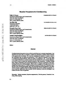
where the jth age group and kth calendar year notation has been substituted by a single indexing over the i = j×k number of cells. Hereafter we shall refer to this model as to the Bayesian AutoRegressive (BAR) model, and compare it to the ’standard’ one stated in (2.3). For computational reasons, Breslow and Clayton (1993) impose constraints on their random effects ui in order that their mean and linear trend are zero, and counter these constraints by introducing a linear term β ′′ k (with k the calendar year), and allowing unrestrained estimation of βj′ . Since we allow free movement of the u’s, we dispense with the linear term, and impose a ’corner’ constraint β1′ = 0. The graph is shown in Figure 1.

Ei-2 Ei-1

b

W Dage[i]

Ei

year[i]

Ei+1 Pi

Ei+2

pyr[i]

casesi

Figure 1: Graphical model for the Bayesian specification, using the directed autoregressive representation.

The model was implemented with WinBugs (Spiegelhalter, Thomas, and Best, 1999), according to the above specification. Goodness-of-fit was assessed through the Deviance Information Criterion (DIC) (Spiegelhalter et al., 2002) for both models.

3 Data We analysed data from the Childhood Cancer Registry of Piedmont (CCRP). The CCRP is the oldest and largest paediatric population-based Cancer Registry active in Italy. Data on incident cases of cancer in children (aged less than 15 years) are available over a 35-year period from 1967 to 2001. Clinical data on diagnosis and treatment are available together with personal information. The criteria for inclusion of cases in the CCRP database have been consistent and the quality of ascertainment has been satisfactory over the period covered by our investigation (Magnani et al., 2003). Counts of new cases of childhood


265

cancer by sex, age class (0, 1-4, 5-9, 10-14 years) and calendar year of diagnosis were used to compute annual incidence rates (per million children per year) referring to the population resident in Piedmont in 1967-2001. We considered the following diagnostic categories: ALL (n = 688), AnLL (n = 145), CNS tumours (n = 753), NB (n = 254), all cancers together (n = 3360). Analyses for ALL and AnLL were limited to 1975-2001 in order to exclude the effect of improvement in diagnostic methods of the early 70’s (Magnani et al., 2003).

4 Results Table 1 presents goodness-of-fit statistics for the standard Poisson and the BAR models, for the cancer types considered in the analysis. Figures 2-4 show observed and expected age-adjusted cancer incidence rates vs. calendar year of diagnosis for all cancer types (Figure 2), CNS tumours and NB (Figure 3) in 1967-2001, and ALL and AnLL in 1975-2001 (Figure 4). Rates expected by BAR are compared to the ones expected by the standard GLM used for cancer trend analysis (Poisson regression). Table 1: Goodness-of-fit statistics for the standard Poisson and the BAR model. p+ D is the Bayesian measure of model dimensionality (Spiegelhalter et al., 2002).

Poisson model

BAR model

Cancer type

DIC

p+ D

DIC

p+ D

ALL

434

7

457

20

AnLL

317

6

331

13

CNS tumours

573

8

596

20

Neuroblastoma

418

6

442

19

All cancer types

842

12

861

24

As expected, given its larger flexibility, BAR displays a more complex behaviour and follows more closely the observed data than the Poisson model. When all cancers are pooled together, the BAR model shows an inflection in the central years of the period under observation (Figure 2), but there are no large differences in the fit achieved (Table 1). For cancers of the nervous system (both CNS tumours and neuroblastoma), expectations do not differ greatly (Figure 3): the Poisson regression and BAR models yield very similar patterns with similar goodness-of-fit (Table 1). For ALL, both the Poisson regression and BAR models again fitted the data quite well, with a slightly smaller error for the BAR model (sum of squared Pearson residuals: Poisson: 1041, BAR: 822). The expectations do not differ greatly for most of the individual years considered, but the overall shape of the models is different (Figure 4). In particu-


266

-6

IR (x 10 person-years)

250

200

Observed BAR Poisson

150

100

50

0 1960

1970

1980

1990

2000

2010

Year of diagnosis

Figure 2: Childhood Cancer Registry of Piedmont. Observed (dots) and expected age - adjusted incidence rates (IR) vs. calendar year of diagnosis for children (0-14 years of age) for all cancer types in 1967-2001. Expectations by the Bayesian autoregressive model (BAR, thick straight line) and the Poisson model (dashed line).

lar, the BAR expected rates do not exhibit a monotonically increasing pattern: in the first half of the study period they oscillate around an average value of 35 cases/106 years, then show a sharp increase in the years from 1989 until 1997, and finally begin to decline from 1998. Figure 4 also shows the corresponding analyses for AnLL (lower curves). For this cancer type, the Poisson and BAR models produced similar patterns.

5 Discussion In this study CCRP data on the incidence of ALL, and other selected childhood cancer sites, were analysed using a Bayesian approach, in order to assess the possibility of a deviation from the monotonic increasing trend necessarily expected by standard regression methods, given their restrictive assumptions. Both the Poisson and BAR models showed increases in incidence for ALL. However, while the former was bound to lead to monotonically increasing rates, the latter’s expectations showed broad oscillations. On the other hand, the two approaches produced very similar patterns for AnLL, nervous system tumours and all cancer types. In standard epidemiological practice, the choice between statistical models is usually carried out through a posteriori criteria, such as goodness-of-fit statistics and residual


70

IR (x 10-6 person-years)

60

267


CNS

50 40 30 20

NB

10 0 1960

1970

1980 1990 Year of diagnosis

2000

2010

Figure 3: Childhood Cancer Registry of Piedmont. Observed (dots) and expected age - adjusted central nervous system tumour (CNS, upper curves) and neuroblastoma (NB, lower curves) incidence rates (IR) vs. calendar year of diagnosis for children (0-14 years of age) in 1967-2001. Expectations by the Bayesian autoregressive model (BAR, thick straight line) and the Poisson model (dashed line).

analysis, and sometimes also a priori considerations about the plausibility of model assumptions. This paper shows an example of the typical pitfall resulting from relying onto a posterior evaluation of the model fit without considering the model assumptions in the first place. In the above application, both the standard Poisson and the BAR model fit the same data equally well (thus providing no useful statistical criteria for the choice of model) and yet for ALL they lead to different interpretations of the shape of the time trends. The Poisson model with fixed-effects only is not an appropriate tool to give a faithful description of the incidence data. Poisson regression fixes the overall shape of the curve, resulting in more weight to long-term trends, while BAR is more flexible and hence more responsive to short-term changes. Besides being more correct for this application, the latter is a safer methodology for descriptive trend analysis, and it might disclose unsuspected behaviour of the disease. Flexible methods (i.e. compatible with non-linear behaviour) are thus capable of providing an ”early warning” of changes in the direction of the incidence trend - high sensitivity. On the other hand, a potential drawback of this and similar methods is that their estimates are very sensitive to short term fluctuations, and may therefore be more susceptible to random variation - low specificity. Bearing these considerations and limitations in mind, the findings presented here are


268

60

IR (x 10-6 person-years)

50


ALL

40 30 20 AnLL

10 0 1960

1970

1980 1990 Year of diagnosis

2000

2010

Figure 4: Childhood Cancer Registry of Piedmont. Observed (dots) and expected age-adjusted acute lymphoblastic leukaemia (ALL, upper curves) and acute non lymphoblastic leukaemia (AnLL, lower curves) incidence rates (IR) vs. calendar year of diagnosis for children (0-14 years of age) in 1975-2001. Expectations by the Bayesian autoregressive model (BAR, thick straight line) and the Poisson model (dashed line).

of interest to epidemiologists since they are consistent with the hypothesis of an infectious aetiology for ALL (Kinlen, 1988; Greaves, 1988; Alexander et al., 1998), given that infections commonly exhibit cyclical behaviour in time, and the short latency time for childhood cancer means that cancers with an infectious aetiology may also be expected to show cyclical time trends. CNS tumours and NB (Figure 3), and AnLL (Figure 4), which are all considered to have a non-infectious aetiology, do not show similar oscillations. Since we do not believe that cancer rates may change at a constant rate over a long period of time, we deem it more appropriate and meaningful to characterise the trend with a nonparametric smoother, which also allows us to detect recent changes in trend.

Acknowledgements This project was partly supported by the special programme ”Ricerca Sanitaria Finalizzata” of the Piedmont Region. We also acknowledge the financial support of the Italian Association for Cancer Research (AIRC) and of the ”Oncology Special Project”, Compagnia di San Paolo FIRMS. The authors would like to thank Franco Merletti, Neil Pearce, Corrado Magnani and Guido Pastore for useful discussions and suggestions.


269

References [1] Aickin, M. (2004): Bayes without priors. J Clin Epidemiol, 57, 4-13. [2] Alexander, F.E., Boyle, P., Carli, P.M., Coebergh, J.W., Draper, G.J., Ekbom, A., Levi, F., McKinney, P.A., McWhirter, W., Magnani, C., Michaelis, J., Olsen, J.H., Peris-Bonet, R., Petridou, E., Pukkala, E., and Vatten, L. (1998): Spatial temporal patterns in childhood leukaemia: further evidence for an infectious origin. EUROCLUS project. Br J Cancer, 77, 812-7. [3] Besag, J., York, J., and Mollie, A. (1991): Bayesian image restoration, with two applications in spatial statistics. Ann Inst Statist Math, 43, 1-59. [4] Box, G.E.P. and Tiao, G.C. (1992): Bayesian Inference in Statistical Analysis. New York: Wiley. [5] Breslow, N.E. and Clayton, D.G. (1993): Approximate inference in Generalised Linear Mixed Models. J Am Stat Assoc, 88, 9-25. [6] Carlin, B.P. and Louis, T.A. (2000): Bayes and Empirical Bayes Methods for Data Analysis. London: Chapman and Hall. [7] Dreifaldt, A.C., Carlberg, M., and Hardell, L. (2004): Increasing incidence rates of childhood malignant diseases in Sweden during the period 1960-1998. Eur J Cancer, 40, 1351-60. [8] Dunson, D.B. (2001): Commentary: practical advantages of Bayesian analysis of epidemiologic data. Am J Epidemiol, 153, 1222-6. [9] Engeland, A., Haldorsen, T., Tretli, S., Hakulinen, T., Horte, L.G., Luostarinen, T., Magnus, K., Schou, G., Sigvaldason, H., Storm, H.H., et al. (1993): Prediction of cancer incidence in the Nordic countries up to the years 2000 and 2010. A collaborative study of the five Nordic Cancer Registries. APMIS Suppl, 38, 1-124. [10] Fahrmeir, L. and Lang, S. (2001): Bayesian inference for generalised additive mixed models based on Markov random field priors. J Roy Stat Soc C-App, 50, 201-20. [11] Greaves, M.F. (1988): Speculations on the cause of childhood acute lymphoblastic leucemia. Leukemia, 2, 120-5. [12] Hjalgrim, L.L., Rostgaard, K., Schmiegelow, K., Soderhall, S., Kolmannskog, S., Vettenranta, K., Kristinsson, J., Clausen, N., Melbye, M., Hjalgrim, H., and Gustafsson, G. (2003): Age- and sex-specific incidence of childhood leukemia by immunophenotype in the Nordic countries. J Natl Cancer Inst, 95, 1539-44. [13] Jowaheer, V. and Sutradhar, B.C. (2002): Analysing longitudinal count data with overdispersion. Biometrika, 89, 389-99. [14] Kinlen, L. (1988): Evidence for an infective cause of childhood leukaemia: comparison of a Scottish new town with a nuclear reprocessing site in Britain. Lancet, 2, 1323-7.

270


[15] Lilford, R.J., Braunholtz, D. (2000): Whos afraid of Thomas Bayes? J Epidemiol Community Health, 54, 731-9. [16] Magnani, C., Dalmasso, P., Pastore, G., Terracini, B., Martuzzi, M., Mosso, M.L., and Merletti, F. (2003): Increasing incidence of childhood leukemia in Northwest Italy, 1975-98. Int J Cancer, 105, 552-7. [17] McCullagh, P. and Nelder, J.A. (1989): Generalised Linear Models (2nd ed.). London: Chapman and Hall. [18] Moller, B., Fekjaer, H., Hakulinen, T., Tryggvadottir, L., Storm, H.H., Talback, M., and Haldorsen T. (2002): Prediction of cancer incidence in the Nordic countries up to the year 2020. Eur J Cancer Prev, 11, S1-96. [19] Ries, L.A.G., Eisner, M.P., Kosary, C.L., Hankey, B.F., Miller, B.A., Clegg, L., Mariotto, A., Feuer, E.J., Edwards, B.K. (Eds) (2004): SEER Cancer Statistics Review, 1975-2001, National Cancer Institute. Bethesda, MD. Available from URL: http://seer.cancer.gov/csr/19752001/. [20] Spiegelhalter, D.J., Thomas, A., and Best, N.G. (1999): WinBUGS Version 1.2 User Manual. MRC Biostatistics Unit. [21] Spiegelhalter, D.J., Best, N.G., Carlin, B.P., and van der Linde, A. (2002): Bayesian measures of model complexity and fit (with discussion). J Roy Statist Soc B, 64, 583-639. [22] Steliarova-Foucher, E., Stiller, C., Kaatsch, P., Berrino, F., Coebergh, J.W., Lacour, B., Parkin, M. (2004): Geographical patterns and time trends of cancer incidence and survival among children and adolescents in Europe since the 1970s (the ACCISproject): an epidemiological study. Lancet, 364, 2097-105.