Nonparametric Bayesian Covariate-Adjusted Estimation of the Youden

Biometrics 000, 000–000

(2017, to appear)

DOI: 000

000 0000

Nonparametric Bayesian Covariate-Adjusted Estimation of the Youden Index

Vanda In´ acio de Carvalho1,⇤ , Miguel de Carvalho1 , and Adam J. Branscum2 1 2

School of Mathematics, University of Edinburgh, Scotland, UK

College of Public Health and Human Sciences, Oregon State University, USA *email: [email protected]

Summary:

A novel nonparametric regression model is developed for evaluating the covariate-specific accuracy of a

continuous biological marker. Accurately screening diseased from nondiseased individuals and correctly diagnosing disease stage are critically important to health care on several fronts, including guiding recommendations about combinations of treatments and their intensities. The accuracy of a continuous medical test or biomarker varies by the cuto↵ threshold (c) used to infer disease status. Accuracy can be measured by the probability of testing positive for diseased individuals (the true positive probability or sensitivity, Se(c), of the test) and the true negative probability (specificity, Sp(c)) of the test. A commonly used summary measure of test accuracy is the Youden index, YI = max{Se(c) + Sp(c)

1 : c 2 R}, which is popular due in part to its ease of interpretation and relevance to

population health research. In addition, clinical practitioners benefit from having an estimate of the optimal cuto↵ that maximizes sensitivity plus specificity available as a byproduct of estimating YI. We develop a highly flexible nonparametric model to estimate YI and its associated optimal cuto↵ that can respond to unanticipated skewness, multimodality and other complexities because data distributions are modeled using dependent Dirichlet process mixtures. Important theoretical results on the support properties of the model are detailed. Inferences are available for the covariate-specific Youden index and its corresponding optimal cuto↵ threshold. The value of our nonparametric regression model is illustrated using multiple simulation studies and data on the age-specific accuracy of glucose as a biomarker of diabetes. Key words: Diagnostic test; Dirichlet process mixtures; Optimal cuto↵; Sensitivity; Specificity.

This paper has been submitted for consideration for publication in Biometrics

Nonparametric Covariate-Adjusted Youden Index

1

1. Introduction Evaluating and ranking the performance of medical tests for screening and diagnosing disease greatly contributes to the health promotion of individuals and communities. The ability of a medical test to distinguish diseased from nondiseased individuals must be thoroughly vetted before the test can be widely used in practice. Throughout this paper we use the terms “medical test” and “test” to broadly include any continuous classifier (e.g., a single biological marker or a composite score from a combination of biomarkers) for a well-defined condition (termed “disease,” with “nondiseased” used to indicate absence of the condition). The ability of a test that produces outcomes on a continuous scale to correctly di↵erentiate between ¯ individuals is characterized by the separation between the diseased (D) and nondiseased (D) ¯ populations. A common parametric approach distributions of test outcomes for the D and D ¯ populations vary according to separate to data analysis assumes that data from the D and D normal distributions. As a safeguard against model misspecification and to permit robustness from the sharp constraints of parametric models (e.g., the normal-normal model) that can fail to accommodate increasingly complex distributions of data from modern medical tests, many contemporary methods for estimating test accuracy are based on flexible statistical models that use nonparametric or semiparametric structures (e.g., Erkanli et al., 2006; Wang et al., 2007; Branscum et al., 2008; Hanson et al., 2008; Gonzalez-Manteiga et al., 2011; In´acio et al., 2011; In´acio de Carvalho et al., 2013; Rodr´ıguez and Mart´ınez, 2014; Zhao et al., 2015). We develop a nonparametric Bayesian regression modeling framework that allows for data-driven flexibility from the confines of parametric models by using dependent Dirichlet process mixtures to estimate the covariate-specific Youden index of a medical test and the covariate-specific optimal threshold to screen individuals in practice. The Youden index (Youden, 1950) is a popular summary measure of the accuracy of ¯ continuous tests. Let yD and yD¯ denote (possibly transformed) data from the D and D

2

Biometrics, 000 0000

populations, respectively, and let FD /fD and FD¯ /fD¯ denote the corresponding continuous distribution/density functions. Without loss of generality, we assume that a subject is classified as diseased (nondiseased) if the test value is greater (less) than a threshold c 2 R. Then, the probability of a positive test for a diseased subject (i.e., the sensitivity of the test) is Se(c) = Pr(yD > c) = 1

FD (c), and the test’s specificity to correctly classify nondiseased

subjects is Sp(c) = Pr(yD¯ 6 c) = FD¯ (c). The Youden index (YI) is given by YI = max{Se(c) + Sp(c) c2R

1} = max{FD¯ (c) c2R

FD (c)},

and thus combines sensitivity and specificity over all thresholds into a single numeric summary. To qualify as a bona fide medical test, it is required that Se(c) + Sp(c) > 1 for all c. Therefore, YI ranges from 0 to 1, with YI = 0 corresponding to complete overlap of the data ¯ populations (i.e., FD (c) = FD¯ (c) for all c) and YI = 1 when the distributions for the D and D distributions are completely separated; values of YI between 0 and 1 correspond to di↵erent levels of stochastic ordering between FD¯ and FD , with values closer to one indicating better discriminatory ability. In addition to providing a global measure of test accuracy, YI provides a criterion to select an optimal threshold to screen subjects in clinical practice. The criterion is to choose the cuto↵ value for which sensitivity plus specificity is maximized, i.e., c⇤ = arg max{FD¯ (c) c2R

FD (c)}.

It is worth noting that the Youden index corresponds to the maximum vertical distance between the receiver operating characteristic (ROC) curve and the chance diagonal line, with c⇤ being the cuto↵ that achieves this maximum. This criterion to select the optimal cuto↵ has been found to be superior to another popular approach for selecting an optimal threshold, namely using the value of c for which the ROC curve is closest to the point (0, 1) in R2 . Specifically, the ROC-based criterion can lead to an increased rate of misclassification compared to the YI-based criterion (Perkins and Schisterman, 2006). The Youden index

Nonparametric Covariate-Adjusted Youden Index

3

continues to be successfully used in practice across a variety of scientific fields (e.g., Hawass, 1997; Demir et al., 2002; Castle et al., 2003; Larner, 2015), resulting in a demand for increased research to develop flexible and robust methods that can reliably estimate it (e.g., Fluss et al., 2005; Molanes-L´opez and L´eton, 2011; Bantis et al., 2014; Zhou and Qin, 2015). Although it is well known that the discriminatory power of a medical test is often a↵ected by covariates, such as age or sex, past research has mostly been devoted solely to estimating the unadjusted Youden index rather than covariate-specific Youden indices and their associated optimal cuto↵s. To the best of our knowledge, the only literature on estimating the covariate-specific YI has involved normal linear regression models (Faraggi, 2003), heteroscedastic kernel-based methods (Zhou and Qin, 2015), and a model-free estimation method (Xu et al., 2014). In this paper, we develop a nonparametric Bayesian regression model that is based on dependent Dirichlet process mixtures, which provide a very flexible tool that can capture a wide variety of functional forms. In contrast with most of the aforementioned models for the Youden index, where only one or two characteristics (mean and/or variance) of the distributions of test outcomes in each group depend on covariates, our modeling framework allows the entire distributions to smoothly change as a function of covariates by using B-splines regression. Therefore, our new procedure successfully combines two sources of nonparametric flexibility, namely (i) arbitrary and unspecified distributions ¯ populations in place of standard parametric for test outcome data from the D and D distributions and (ii) nonparametric regression B-splines in place of the standard linearity assumption in multiple regression. The remainder of the paper is organized as follows. In the next section we introduce our new approach to nonparametric Bayesian estimation of the Youden index via a flexible mixture model. The performance of our methods is assessed in Section 3 using multiple simulation

4

Biometrics, 000 0000

studies. Section 4 applies our methods to estimate the age-specific accuracy of glucose as a biomarker of diabetes. Concluding remarks are provided in Section 5.

2. Models and Methods We develop a nonparametric regression model to estimate the covariate-specific Youden index and optimal threshold by using dependent Dirichlet process (DDP) mixtures. The Dirichlet process (Ferguson, 1973) is a prior probability model for an unknown distribution function F and is characterized by a baseline distribution F ⇤ (the prior mean; E{F (·)} = F ⇤ (·)) and a positive precision parameter ↵ that is related to the prior variance, with larger values of ↵ resulting in prior realizations of F that are stochastically closer to F ⇤ . Let F ⇠ DP(↵, F ⇤ ) denote that F follows a Dirichlet process prior with parameters ↵ and F ⇤ . We will use the following constructive definition of the Dirichlet process developed by Sethuraman (1994): F (·) =

1 X

p`

✓` (·).

`=1

Here,

✓

denotes a point mass at ✓, and ✓1 , ✓2 , . . . are independently distributed according to

F ⇤ and they are independent of the weights, which are generated by a stick-breaking scheme Q iid wherein p1 = q1 and for ` = 2, 3, . . ., p` = q` `r=11 (1 qr ), with q1 , q2 , . . . ⇠ Beta(1, ↵).

MacEachern (2000) proposed the DDP, a generalization of the DP, as a prior for a collection of covariate-dependent random distributions {Fx : x 2 X ✓ Rp }. Because of the full support properties it obtains (Barrientos et al., 2012), we consider a ‘single-weights’ DDP (De Iorio et al., 2009) in which Fx (·) =

1 X

p`

✓x` (·).

(1)

`=1

The random support locations ✓x` = {✓l (x) : x 2 X } are, for ` = 1, 2, . . ., independent and identically distributed realizations from a stochastic process over the covariate space X and the weights {p` }1 `=1 match those from a standard DP. We begin by describing a nonparametric model for medical test data in the absence of covariates and build up to

Nonparametric Covariate-Adjusted Youden Index

5

our new nonparametric DDP mixture model that contains nonlinear regression B-splines for capturing unforeseen complex covariate trends and that provides robust subpopulationspecific inference about YI.

2.1 Nonparametric Model In the absence of covariates, we consider nonparametric data analysis using separate Dirichlet process mixture (DPM) models for data yD1 , . . . , yDnD from population D and yD1 ¯ , . . . , yDn ¯ ¯ D ¯ That is, we consider normal mixture models with a DP prior placed on from population D. the mixing distribution, namely iid

yDi |FD ⇠ FD , where (c; µ,

2

FD (c) =

Z

(c; µ,

2

)dGD (µ,

2

GD ⇠ DP(↵D , G⇤D ),

),

) denotes the normal distribution function with mean µ and variance

is evaluated at c. We select the baseline distribution G⇤D (µ, aD , bD ) (i.e., G⇤D (µ,

2

2

2

) to be N(µ | mD , s2D ) (

that 2

|

) is the product of independent normal and gamma distribution func-

¯ population. The stick-breaking tions). A similar model is posited for data from the D representation of the Dirichlet process leads to specifying the sampling models as infinite normal mixtures given by FD (c) =

1 X

pD` (c; µD` ,

`=1

2 D` )

and FD¯ (c) =

1 X

pD` (c; µD` ¯ ¯ ,

2 ¯ ), D`

`=1

with the aforementioned Sethuraman construction used to define the weights and priors (e.g., iid

iid

µD` ⇠ N(mD , s2D ) and D`2 ⇠ (aD , bD )). The Youden index under this nonparametric model P 2 2 ⇤ is YI = maxc2R { 1 (c; µD` ¯ ¯ , D` ¯ ) pD` (c; µD` , D` ))} and c is the input that returns `=1 (pD` the maximum value. Following the popular computational approach by Ishwaran and James

(2002), we fit the model by accurately approximating the infinite mixtures that characterize FD and FD¯ by finite mixtures with many components (details in Section 2.2).

6

Biometrics, 000 0000

2.2 Nonparametric Regression Model We develop a robust nonparametric model that can be used to determine if and how the accuracy of a medical test varies across subpopulations defined by di↵erent covariate values. For ease of exposition, we assume that p = 1 (i.e., one covariate); an extension to the multiple covariate case is outlined at the end of this section. In this setting, sensitivity and specificity depend on a single covariate x, so that Se(c | x) = Pr(yD > c | x) = 1

FD (c | x) and Sp(c |

x) = Pr(yD¯ 6 c | x) = FD¯ (c | x). The data from population D are {(yDi , xDi ) : i = 1, . . . , nD } ¯ we have {(yDj and from population D ¯ , xDj ¯ ) : j = 1, . . . , nD ¯ }, where xDi , xDj ¯ 2 X ✓ R for ind.

all i, j. Test outcomes are assumed to be independent with yDi | xDi ⇠ FD ( · | xDi ) and ind.

yDj ¯ | xDj ¯ ⇠ FD ¯ ( · | xDj ¯ ). For x 2 X , the covariate-specific Youden index and optimal cuto↵ are given by YI(x) = max{FD¯ (c | x) c2R

FD (c | x)} and c⇤ (x) = arg max{FD¯ (c | x) c2R

FD (c | x)}.

(2)

Note that we can also estimate YI(xD , xD¯ ) and c⇤ (xD , xD¯ ), the Youden index and optimal cuto↵ for diseased subjects with covariate xD and nondiseased subjects with covariate xD¯ . We specify a prior probability model for the entire collection of conditional distributions ¯ where the conditional distributions in each Fd = {Fd ( · | x) : x 2 X } for d 2 {D, D}, population are characterized by covariate-dependent mixtures of normals Z ¯ Fd (c | x) = (c; µ, 2 )dGdx (µ, 2 ), d 2 {D, D},

(3)

with the single weights DDP prior in (1) placed on the mixing measure Gdx (·). Specifically, we set ✓d` (x) = (µd` (x),

2 d` ),

where the potentially nonlinear function µd` (x) is approximated

by a linear combination of cubic B-spline basis functions over a sequence of knots ⇠d0 < ⇠d1 < · · · < ⇠dK < ⇠d,K+1 . The knots ⇠d0 and ⇠d,K+1 are boundary knots and ⇠d1 , . . . , ⇠dK are interior knots. Thus, µd` (x) =

Q X q=1

d`q Bdq (x),

Q = K + 4,

(4)

Nonparametric Covariate-Adjusted Youden Index

7

where Bdq (x) corresponds to the qth cubic B-spline basis function in group d evaluated at x. ¯ groups. For simplicity, we have assumed the same number of interior knots for the D and D An important issue regarding the application of regression splines is the selection of interior knots, i.e., the number of inner knots and their location. As stated in Durrleman and Simon (1989), in practice often only a few knots are needed to adequately describe most of the phenomena likely to be observed in medical studies. A maximum of three or four interior knots will often suffice. The selection of K can be assisted by a model selection criterion, e.g., the log pseudo marginal likelihood (LPML) (Geisser and Eddy, 1979). We use empirical percentiles of xd to determine knot locations. Specifically, following Rosenberg (1995), the covariate space is partitioned in accordance with the goal of having each interval containing approximately the same number of observations, which leads to setting ⇠dk equal to the ¯ and k = 1, . . . , K. The boundary knots are set k/(K + 1) percentile of xd , for d 2 {D, D} equal to the minimum and maximum of xd . We proceed by noting that µd` (x) can be written as µd` (x) =

Q X

d`q Bdq (x)

= zTd

d` ,

q=1

where zd = (Bd1 (x), . . . , BdQ (x)) and T

d`

=(

d`1 , . . . ,

d`Q )

T

. Thus, under this formulation,

the base stochastic processes are replaced with a group-specific base distribution G⇤d that generates the component specific regression coefficients and variances. The B-splines DDP mixture model can therefore be represented as a DP mixture of Gaussian regression models where the component means vary nonlinearly with the predictors, namely Z ¯ Fd (c | x) = (c; zTd , 2 )dGd ( , 2 ), Gd ⇠ DP(↵d , G⇤d ), d 2 {D, D}. To complete model (5), we take G⇤d ( ,

2

2

) to be NQ ( | md , S d ) (

hyperpriors md ⇠ NQ (md0 , S d0 ) and S d 1 ⇠ WishartQ (⌫d , (⌫d with degrees of freedom ⌫d and expectation

1 d

d)

1

(5)

| ad , bd ), with conjugate

) (a Wishart distribution

).

We use the blocked Gibbs sampler of Ishwaran and James (2002) for posterior sampling.

8

Biometrics, 000 0000

The blocked Gibbs sampler relies on truncating the stick-breaking representation to a finite number of components. Hence, FD (c | x) =

LD X

T

pD` (c; zD

D` ,

2 D` )

`=1

and FD¯ (c | x) =

LD ¯ X

pD` (c; zTD¯ ¯

¯ , D`

2 ¯ ), D`

(6)

`=1

with LD and LD¯ being upper bounds on the number of components used for the approximations. The conditional distribution in each group is then estimated by a finite mixture of Gaussian regression models with the mixing weights automatically determined by the data. The weights pd` are generated from the stick-breaking representation, while iid d`

⇠ NQ (md , S d ) and

2 iid d` ⇠

(ad , bd ). The full conditional distributions have the conjugate

forms detailed in Appendix A of the Supplementary Materials. The level of truncation can P be guided by properties of Ud = 1 `=Ld +1 pd` . Ishwaran and Zarepour (2000) demonstrated that E(Ud ) = ↵dLd /(1 + ↵d )Ld and var(Ud ) = ↵dLd /(2 + ↵d )Ld

↵d2Ld /(1 + ↵d )2Ld . For example,

¯ as in our simulation study and application, results setting Ld = 20 and ↵d = 1 (d 2 {D, D}) in E(Ud ) = 10

6

. and var(Ud ) = 10

10

, which is more than adequate for our data analysis.

Posterior inference for YI(x) is obtained by using (2) and (6), and the covariate-specific optimal cuto↵ c⇤ (x) is the input that returns the maximum. A grid search was used to identify the maximum. Finally, in the case of multiple covariates (so that x 2 Rp ), a possibility would be to use the additive structure µd` (x) = fd`1 (x1 ) + · · · + fd`p (xp ). The model can therefore be regarded as a DDP mixture of additive models. Each function could be approximated by basis functions as in (4). 2.3 Theoretical Properties In this section we characterize the support properties of our nonparametric models, with and without covariates. The overarching goal is to construct extremely flexible models for FD and FD¯ that support any collection of Youden indexes with positive probability. Roughly speaking, the following results are an affirmation of the theoretical resilience of the model, in

Nonparametric Covariate-Adjusted Youden Index

9

the sense that the model can successfully adapt to and support very complex distributions of data. We have the following theorem about the nonparametric model in Section 2.1. Theorem 1:

Let (⌦, A, P ) be the probability space associated with the DPM model,

which induces the Youden index YI = maxc2R {FD¯ (c)

FD (c)}. For almost every ! 2 ⌦,

let YI! be a realization of the Youden index under the proposed DPM. Then, for every " > 0, it holds that P (! 2 ⌦ : |YI!

YI| < ") > 0.

The following analogous result holds for the covariate-dependent nonparametric regression setting in Section 2.2. Theorem 2:

Let (⌦, A, P ) be the probability space associated with the general DDP

mixture of Gaussian distributions in (3) with the single weights DDP prior in (1) placed on the mixing measure and with trajectories given by YI(x) = maxc2R {FD¯ (c | x)

FD (c | x)}.

For almost every ! 2 ⌦ and every x 2 X , let YI! (x) be a trajectory of the Youden index under the DDP mixture model. Then, for x1 , . . . , xn 2 X , for every positive integer n and " > 0, it holds that P (! 2 ⌦ : |YI! (xi )

YI(xi )| < ", i = 1, . . . , n) > 0.

Proofs are given in Appendix B of the Supplementary Materials.

3. Simulation Study To evaluate the performance of our nonparametric regression model for estimating the covariate-specific Youden index and optimal cuto↵ value, we analyzed simulated data under the following four scenarios: linear mean, a mixture of linear means, nonlinear mean with constant variance, and nonlinear mean with covariate-dependent variance. For each scenario, 100 data sets were generated using sample sizes of (nD , nD¯ ) = (100, 100), (nD , nD¯ ) = (100, 200), and (nD , nD¯ ) = (200, 200). For all scenarios, covariate values were independently generated from a uniform distribution, namely xDi ⇠ U(0, 1) and xDj ¯ ⇠ U(0, 1).

10

Biometrics, 000 0000

3.1 Simulation Scenarios In Scenario 1, we consider di↵erent homoscedastic linear mean regression models for the diseased and nondiseased groups. Specifically, independent data were generated as yDi | xDi ⇠ N(2+4xDi , 22 ),

2 yDj ¯ | xDj ¯ ⇠ N(0.5+xDj ¯ , 1.5 ),

i = 1, . . . , nD ,

j = 1, . . . , nD¯ .

The primary purpose of including this scenario is to investigate the loss of efficiency of our covariate-specific Youden index and optimal cuto↵ estimators when standard parametric assumptions hold. ¯ populations is The popular normal-normal regression model for data from the D and D violated in Scenarios 2-4. Data for Scenario 2 are governed by the following mixtures of homoscedastic linear mean regression models: ind.

yDi | xDi ⇠ 0.5N(2 + 3xDi , 12 ) + 0.5N(6 + 2.5xDi , 12 ), ind.

2 2 yDj ¯ | xDj ¯ ⇠ 0.5N(2 + xDj ¯ , 1.25 ) + 0.5N( 2.5 + xDj ¯ , 1 ).

Scenario 3 involves the homoscedastic nonlinear mean regression models given by ind.

ind.

2 2 yDi | xDi ⇠ N(9+1.15x2Di , 2.52 ) and yDj ¯ | xDj ¯ ⇠ N(5.5+1.75xDj ¯ +1)), 1.5 ), ¯ +1.5 sin(⇡(xDj

for i = 1, . . . , nD , and j = 1, . . . , nD¯ . Finally, in Scenario 4, the most complex scenario considered, we use the following heteroscedastic nonlinear mean regression models for the diseased and nondiseased groups: ind.

yDi | xDi ⇠ N(5 + 1.5xDi + 1.5 sin(xDi ), 1.5 + (10xDi

2)),

ind.

yDj ¯ | xDj ¯ ⇠ N(3 + 1.5 sin(⇡xDj ¯ ), 0.2 + exp(xDj ¯ )). 3.2 Models For each simulated data set we fit the B-splines DDP mixture model with Q = 4, thus ¯ equal to one, which corresponding to K = 0 (no interior knots). We set ↵d (d 2 {D, D}) according to Hanson (2006) is the default value in the absence of prior information on the number of components needed to adequately describe Fd ( · | x). Using results from Antoniak

Nonparametric Covariate-Adjusted Youden Index

11

(1974) and Escobar (1994), this choice leads to a prior expected number of components of 5 when nd = 100 and 6 when nd = 200. For the normal-gamma prior we set md0 = 0Q , S d0 = 100IQ , ⌫d = Q + 2,

1 d

= IQ , where IQ denotes the Q ⇥ Q identity matrix, and we used

ad = bd = 0.1. The normal prior for

d`

is relatively di↵use since variances in S d0 are large

and the degree of freedom in the Wishart prior is small. Although the gamma prior for

2 d`

has a peak at 0+ , we found that estimates of the Youden index and optimal cuto↵ were robust to moderate departures from this prior distribution. We capped the maximum number of mixture components at Ld = 20 and, thus, a maximum of 20 regression models was used to approximate the conditional distributions in (5). We compared our estimator to results from ordinary linear regression analysis, i.e., where ⇤ D,

FD (c | x⇤ ) = (c; x⇤T T

⇤ d

with x⇤ = (1, x) and

=(

⇤ d0 ,

2⇤ D)

⇤ T d1 ) ,

and FD¯ (c | x⇤ ) = (c; x⇤T

⇤ ¯, D

2⇤ ¯ ) D

¯ We used the following priors that align d 2 {D, D}.

with those from the nonparametric analysis: ⇤ d

⇠ N2 (m⇤d , S ⇤d ),

2⇤ d

⇠ (a⇤d , b⇤d ),

m⇤d ⇠ N2 (m⇤d0 , S ⇤d0 ),

S ⇤d

1

⇠ Wishart(⌫d⇤ , (⌫d⇤

⇤ 1 d ) ),

with m⇤d0 = 02 ,

S ⇤d0 = 100I2 ,

⌫d⇤ = 4,

(

⇤ 1 d)

= I2 ,

and a⇤d = b⇤d = 0.1.

This model can be regarded as a Bayesian version of the model considered by Faraggi (2003). In both cases 1000 samples were kept after a burn-in period of 500 iterations of the Gibbs sampler. In addition, we compared our model to the nonparametric kernel-based method of Zhou and Qin (2015) (details appear in Section C of the Supplementary Materials).

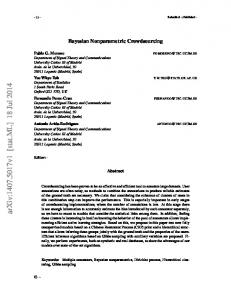
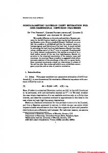
3.3 Results The estimated covariate-specific Youden index and optimal cuto↵ functions along with the 2.5 and 97.5 percentiles in Figures 1 and 2 illustrate the ability of our model to accurately and precisely capture complex functional forms dynamically. Specifically, for the case (nD , nD¯ ) =

12

Biometrics, 000 0000

(100, 200), which is similar to the diabetes application in Section 4, the minor loss in efficiency for our nonparametric estimator when a parametric normal linear regression holds (panels (a) and (e) in Figures 1 and 2) is a small price to pay for the benefit of the extreme robustness that leads to accurate data-driven estimates under increasingly complex scenarios (remaining panels in Figures 1 and 2). Similar conclusions were found for the other sample sizes (Figures 1–8 in Appendix C of the Supplementary Materials). As indicated by these figures, our estimator is able to successfully recover the true functional form of both the Youden index and optimal cuto↵ for all scenarios considered. As expected, the estimator based on the normality assumption has the best performance in Scenario 1, but it is unsuitable for the remaining scenarios and, unlike our nonparametric estimator, its performance fails to improve as the sample size increases. It is noteworthy that, in all scenarios considered, posterior uncertainty decreases as sample size increases and that even with a relatively low sample size combination of (nD , nD¯ ) = (100, 100), our method performs very well. The kernel-based estimator is also able to successfully recover the true functional form of the Youden index and optimal cuto↵. The discrepancy between estimated and true Youden index and optimal cuto↵ was assessed using the empirical global mean squared error (EGMSE) EGMSEYI

nx 1 X c r) = {YI(x nx r=1

YI(xr )}2 ,

where nx = 11 and the xr ’s are evenly spaced over [0, 1]. An analogous expression follows for EGMSEc⇤ . Boxplots summarizing the distribution of EGMSE are presented in Figures 9 and 10 of the Supplementary Materials. For most sample sizes considered under these scenarios, our B-splines DDP estimator produced smaller EGMSE compared to the kernel estimator (especially for the optimal cuto↵). The mean LPML values and 90% intervals presented in Table 1 of the Supplementary Materials highlight the performance of our model compared to the normal regression model.

Nonparametric Covariate-Adjusted Youden Index

13

The conditional predictive ordinate (CPO) was calculated using M post burn-in Gibbs sampler iterates (each of which is indexed by the superscript (k) in the following formula for CPO): LPMLD =

nD X

log(CPODi ),

CPODi1

i=1

An analogous formula holds for LPMLD¯ .

(L M D ⇣ 1 X X (k) = p yDi ; zTDi M k=1 `=1 D`

(k) (k) 2 D` , ( D` )

⌘

)

.

As suggested by a referee, we also fit the B-splines DDP model using multiple interior knots (Q = 7). The estimated Youden index and optimal cuto↵ functions are shown in Figures 1–8 of the Supplementary Materials. The true functional form is recovered successfully for both YI(x) and c⇤ (x), although with higher posterior uncertainty than with Q = 4. The model with Q = 4 was clearly favored by LPML for the majority of the scenarios and sample sizes considered (results not shown). [Figure 1 about here.] [Figure 2 about here.]

4. Application Diabetes mellitus, a chronic disease characterized in part by high levels of blood sugar (glucose), is an increasingly serious global health concern, with the estimated worldwide prevalence of 8% expected to continue to rise (Shi and Hu, 2014). A population-based survey of diabetes in Cairo, Egypt collected data on postprandial blood glucose measurements that were obtained from a finger stick on 286 adults. Our primary goal is to evaluate the agespecific accuracy of glucose to serve as a biomarker of diabetes. Based on the World Health Organization diagnostic criteria for diabetes, 88 subjects were classified as diabetic and 198 as nondiabetic (Smith and Thompson, 1996). Density estimates from an unadjusted analysis of data from the diabetic and nondiabetic groups using histograms of glucose levels and the DPM mixture of normal models described

14

Biometrics, 000 0000

in Section 2.1 are presented in Figures 11 (a) and (b) of the Supplementary Materials; Figure 11 (c) presents estimates of the distribution functions and optimal cuto↵ value. The Bayesian nonparametric estimate of the unadjusted Youden index (95% probability interval) of 0.66 (0.56, 0.75) illustrates the reasonably strong overall discriminatory ability of glucose to correctly classify diabetes status. The optimal cuto↵ that maximizes test accuracy occurs at a glucose level of 127 mg/dL (118, 142). The aging process may be associated with relative insulin resistance among those who are nondiabetic (Smith and Thompson, 1996). Thus, there is a need to accurately estimate the Youden index and optimal cuto↵ value adjusted for age. Our B-splines DDP mixture model was applied to the glucose data with Q = 4, 5, 6, and 7 and the same di↵use prior specification described in Section 3.2. Posterior inference was based on estimates calculated from 3500 Gibbs sampler iterates after a burn-in of the first 1500 realizations was discarded. Glucose levels were scaled by dividing by the standard deviation to fit the model, but we transformed back to the original scale to present the results (hyperparameter specification was made on the scaled data). Plots of the B-splines basis functions in each group are presented in Figure 12 of the Supplementary Materials. Figure 3 presents the posterior mean of the Youden index and the optimal cuto↵ for the di↵erent values of Q as a function of age, along with a band constructed using the pointwise 2.5% and 97.5% posterior quantiles. To enable comparisons across Q, Figure 13 of the Supplementary Materials shows the 4 posterior means together on the same graph. Our analysis found that glucose is a more accurate biomarker of diabetes in younger adult populations, with its accuracy decreasing with age and the optimal cuto↵ increasing with age. Also, as expected, posterior uncertainty increases with Q. The LPML values for models applied to the nondiabetic data are

878,

880,

881, and

887 for Q = 4, 5, 6, and 7,

Nonparametric Covariate-Adjusted Youden Index

respectively, while for the diabetic population the corresponding LPML values are 532,

531, and

15

530,

532.

Age-specific nonparametric estimates of the Youden index and optimal cuto↵ (posterior mean and 95% probability bands) when Q = 4 along with unadjusted estimates of YI and c⇤ are presented in Figures 4 (a) and (b). The probability band for the optimal cuto↵ from the unadjusted analysis is not completely contained in the age-adjusted band, which gives some additional support for estimating the age-specific accuracy of glucose for diagnosing diabetes. We compared estimates from our B-splines DDP model to those from the Gaussian linear regression model in Section 3.2 (Figures 4 (c) and (d)). To facilitate comparisons, Figures 4 (e) and (f) present the estimates together for both methods. While the estimates of the Youden index are similar, the di↵erent methods provide di↵erent estimates of the optimal age-specific cuto↵ values. For the nondiabetic group, the B-splines DDP model has LPML equal to -878 compared to -935 under the normal model, while for the diabetic group the corresponding LPML values are -530 and -532. The pseudo Bayes factors, which are larger than 1020 and 7, support the nonparametric model for both groups, although just slightly for the diabetic group. A log transformation made the normal model slightly more competitive, although the B-splines DDP mixture model was still preferred in the nondiseased group; for the diabetic group the comparison was roughly unchanged. We also highlight the important finding that our nonparametric analysis did not produce a substantial increase in the uncertainty associated with the estimates of the Youden index and optimal cuto↵ in this setting. A comparison with the kernel approach is presented in Figure 14 in the Supplementary Materials. A sensitivity analysis with a data-driven prior (Section D and Figure 15 of the Supplementary Materials) resulted in similar inferences as the primary analysis.

[Figure 3 about here.]

16

Biometrics, 000 0000

[Figure 4 about here.]

5. Concluding Remarks We developed a Bayesian nonparametric regression model to estimate the covariate-specific Youden index and the corresponding optimal cuto↵ value. The flexibility of our model arises from using dependent Dirichlet process mixtures combined with B-splines regression. Our simulation study illustrated the ability of the model to dynamically respond to complex data distributions in a variety of scenarios, with little price to be paid in terms of decreased posterior precision for the extra generality of our nonparametric estimator when compared with parametric estimates (even when the parametric model holds). Our investigation into the potential of glucose to serve as a biomarker of diabetes found that its classification accuracy decreases with age and the optimal cuto↵ to screen subjects in practice increases with age. It is important to underscore that, although the Youden index gives equal weight to sensitivity and specificity, a weighted Youden index can also be used. For instance, weighting by the prevalence of disease in the population would emphasize test sensitivity over specificity when the disease is common. An interesting avenue for future research is variable selection in the diseased and nondiseased subpopulations; spike and slab priors could be a possible approach to this problem.

6. Supplementary Materials Supplementary Materials describing the Gibbs sampling algorithm for fitting the nonparametric regression model, proofs of Theorems 1 and 2, details on the nonparametric kernel method of Zhou and Qin (2015), and the additional figures referenced in Sections 3 and 4 are available at the Biometrics website on Wiley Online Library.

Nonparametric Covariate-Adjusted Youden Index

17

Acknowledgements We thank a referee for suggestions that greatly improved the paper. This research was partially funded by CONICYT, through the Fondecyt projects 11130541 and 11121186.

References Antoniak, C. E. (1974). Mixtures of Dirichlet processes with applications to Bayesian nonparametric problems Annals of Statistics 2, 1152–1174. Bantis, L. E., Nakas, C. T., and Reiser, B. (2014). Construction of confidence regions in the ROC space after the estimation of the optimal Youden index-based cut-o↵ point. Biometrics 70, 212–223. Barrientos, A. F., Jara, A., and Quintana, F. (2012) On the support of MacEachern’s dependent Dirichlet processes and extensions. Bayesian Analysis 7, 277–310. Branscum, A.J., Johnson, W.O., Hanson, T.E., and Gardner, I.A. (2008). Bayesian semiparametric ROC curve estimation and disease diagnosis. Statistics in Medicine 27, 2474–2496. Castle, P., Lorincz, A. T., Scott, D. R., Sherman, M. E., Glass, A. G., Rush, B. B. et al. (2003). Comparison between prototype hybrid capture 3 and hybrid capture 2 human papillomavirus DNA assays for detection of high-grade cervical inter epithelial neoplasia and cancer. Journal of Clinical Microbiology 9, 4022–4030. Demir, A., Yaral, N., Fisgir, T., Duru, F., and Kara, A. (2002). Most reliable indices in di↵erentiation between thalassemial trait and iron deficiency anemia. Pedriatics International 44, 612–616. De Iorio, M., Johnson, W. O., M¨ uller, P. and Rosner, G. L. (2009). Bayesian nonparametric non-proportional hazards survival modelling. Biometrics 65, 762–771. Durrleman, S. and Simon, R. (1989). Flexible regression models with cubic splines. Statistics in Medicine 8, 551–561.

18

Biometrics, 000 0000

Erkanli, A., Sung, M., Costello, E. J., and Angold, A. (2006). Bayesian semi-parametric ROC analysis. Statistics in Medicine 25, 3905–3928. Escobar, M. D. (1994). Estimating normal means with a Dirichlet process prior. Journal of the American Statistical Association 89, 268–277. Faraggi, D. (2003). Adjusting receiver operating characteristic curves and related indices for covariates. Journal of the Royal Statistical Society, Ser. D 52, 1152–1174. Ferguson, T. S. (1973). A Bayesian analysis of some nonparametric problems. Annals of Statistics 1, 209–230. Fluss, R., Faraggi, D., and Reiser, B. (2005). Estimation of the Youden index and its associated cuto↵ point. Biometrical Journal 47, 458–472. Geisser, S., and Eddy, W. (1979). A predictive approach to model selection. Journal of the American Statistical Association 74, 153–160. Gonzalez-Manteiga, W., Pardo-Fernandez, J. C., and Van Keilegom, I. (2011). ROC curves in non-parametric location-scale regression models. Scandinavian Journal of Statistics 38, 169–184. Hanson, T. E. (2006). Modeling censored lifetime data using a mixture of gammas baseline. Bayesian Analysis 1, 575–594. Hanson, T. E., Branscum, A. J., and Gardner, I. A. (2008). Multivariate mixtures of Polya trees for modelling ROC data. Statistical Modelling 8, 81–96. Hawass, N. E. D. (1997). Comparing the sensitivities and specificities of two diagnostic procedures performed on the same group of patients. The British Journal of Radiology 70, 360–366. In´acio, V., Turkman, A. A., Nakas, C. T., and Alonzo, T. A. (2011). Nonparametric Bayesian estimation of the three-way receiver operating characteristic surface. Biometrical Journal 53, 1011–1024.

Nonparametric Covariate-Adjusted Youden Index

19

In´acio de Carvalho, V., Jara, A., Hanson, T. E., and de Carvalho, M. (2013). Bayesian nonparametric ROC regression modeling. Bayesian Analysis 8, 623–646. Ishwaran, H., and James, L. F. (2002). Approximate Dirichlet process computing in finite normal mixtures: smoothing and prior information. Journal of Computational and Graphical Statistics 11, 508–532. Ishwaran, H., and Zarepour, M. (2000). Markov chain Monte Carlo in approximate Dirichlet and beta two-parameter process hierarchical models. Biometrika 87, 371–390. Larner, A. J. (2015). Diagnostic Test Accuracy Studies in Dementia: A Pragmatic Approach. Cham: Springer. MacEachern, S. N. (2000). Dependent Dirichlet processes. Technical Report, Department of Statistics, The Ohio State University. Molanes-L´opez, E. M., and Let´on, E. (2011). Inference of the Youden index and associated threshold using empirical likelihood quantiles. Statistics in Medicine 30, 2467–2480. Perkins, N. J., and Schisterman, E. J. (2006). The inconsistency of “optimal” cut-points using two ROC based criteria. American Journal of Epidemiology 163, 670–675. Rodr´ıguez, A., and Mart´ınez, J. C. (2014). Bayesian semiparametric estimation of covariatedependent ROC curves. Biostatistics 2, 353–369. Rosenberg, P. S. (1995). Hazard function estimation using B-splines. Biometrics 51, 874–887. Sethuraman, J. (1994). A constructive definition of the Dirichlet process prior. Statistica Sinica 2, 639–650. Schisterman, E. F., and Perkins, N. (2007). Confidence intervals for the Youden Index and corresponding optimal cut-point. Communications in Statistics: Simulation and Computation 36, 549–563. Shi, Y., and Hu, F.B. (2014). The global implications of diabetes and cancer. The Lancet 383, 1947–1948.

20

Biometrics, 000 0000

Smith, P. J., and Thompson, T. J. (1996). Correcting for confounding in analyzing receiver operating characteristic curves. Biometrical Journal 7, 857–863. Wang, C., Turnbull, B. W., Gr¨ohn, Y. T., and Nielsen, S. S. (2007). Nonparametric estimation of ROC curves based on Bayesian models when the true disease state is unknown. Journal of Agricultural, Biological, and Environmental Statistics 12, 128–146. Xu, T., Wang, J., and Fang, Y. (2014). A model-free estimation for the covariate-adjusted Youden index and its associated cut-point. Statistics in Medicine 33, 4963–4974. Youden, W. J. (1950). Index for rating diagnostic tests. Cancer 3, 32–35. Zhao, L., Feng, D., Chen, G., and Taylor, J. M. G. (2005). A unified Bayesian semiparametric approach to assess discrimination ability in survival analysis. Biometrics 72, 554–562. Zhou, H., and Qin, G. (2015). Nonparametric covariate adjustment for the Youden index. In Applied Statistics in Biomedicine and Clinical Trials Design, 109–132, Cham: Springer.

0.8

1.0

0.4

0.6

0.8

1.0

1.0 0.6 0.4

Youden index

0.2 0.2

0.4

0.6

0.8

1.0

0.0

0.2

0.4

0.6

(b)

(c)

(d)

0.6

0.8

1.0

0.0

0.2

0.4

0.6

0.8

1.0

0.6

0.8 0.4

0.6

0.8

1.0

0.0

0.2

0.4

0.6

(f)

(g)

(h)

0.0

0.2

0.4

0.6

0.8

1.0

0.8 0.6 0.0

0.2

0.4

Youden index

0.8 0.6 0.0

0.2

0.4

Youden index

0.8 0.6 0.0

0.2

0.4

Youden index

0.8 0.6 0.4

1.0

1.0

(e)

1.0

x

1.0

x

0.8

1.0

0.2 0.2

x

0.6

0.8

0.0 0.0

x

0.4

1.0

0.4

Youden index

0.8 0.6 0.0

0.2

0.4

Youden index

0.8 0.6 0.0

0.2

0.4

Youden index

0.8 0.6 0.4

0.4

0.8

1.0

(a)

1.0

x

0.2

0.2

0.0 0.0

x

0.0 0.0

0.8

1.0 0.2

x

0.0

0.2

0.6 0.2 0.0

0.0

1.0

0.0

0.4

Youden index

0.8

1.0 0.8 0.6

21

x

0.2

Youden index

0.6 0.2 0.0

0.4

1.0

0.2

1.0

0.0

Youden index

0.4

Youden index

0.6 0.4 0.0

0.2

Youden index

0.8

1.0

Nonparametric Covariate-Adjusted Youden Index

0.0

0.2

0.4

0.6

0.8

1.0

0.0

0.2

0.4

0.6

x

x

x

x

(i)

(j)

(k)

(l)

0.8

1.0

Figure 1: True (solid black lines) and the average value over 100 simulated data sets (dashed blue lines) of the posterior mean (for the Bayesian estimators) of the Youden index function for the sample size (nD , nD¯ ) = (100, 200). A band constructed using the pointwise 2.5% and 97.5% quantiles across simulations is presented in gray. Row 1: B-splines DDP estimator. Row 2: Normal estimator. Row 3: Kernel estimator . Panels (a), (e), and (i) show the results under Scenario 1, panels (b), (f), and (j) under Scenario 2, panels (c), (g), and (k) under Scenario 3, and panels (d), (h), and (l) under Scenario 4.

6.5

Biometrics, 000 0000

0.4

0.6

0.8

1.0

0.0

0.2

0.4

0.6

0.8

1.0

0.0

0.2

0.4

0.6

0.8

(c)

(d)

1.0

0.0

0.2

0.4

0.6

0.8

1.0

5.5 5.0 4.5

Optimal cutoff 0.2

0.4

0.6

0.8

1.0

0.0

0.2

0.4

0.6

x

x

(e)

(f)

(g)

(h)

1.0

5.5 5.0 4.5

Optimal cutoff

3.5 3.0

6 0 0.8

4.0

9

1

7

8

Optimal cutoff

3 2

Optimal cutoff

4

4

10

6.0

5

5

11

6.5

x

0.6

1.0

3.5 0.0

x

0.4

0.8

3.0

6 0.8

4.0

10 9 7

8

Optimal cutoff

4 3 2

Optimal cutoff

1 0 0.6

1.0

6.0

5

5 4 Optimal cutoff

3

0.4

0.8

6.5

(b)

3

Optimal cutoff

0.6

(a)

2

0.2

0.4 x

1 0.0

0.2

x

2

0.2

5.5 0.0

x

1 0.0

5.0

1.0

x

11

0.2

4.5

Optimal cutoff

3.5 3.0

0 0.0

4.0

9 6

1

1

7

8

Optimal cutoff

3 2

Optimal cutoff

3 2

Optimal cutoff

4

4

10

6.0

5

5

11

22

0.0

0.2

0.4

0.6

0.8

1.0

0.0

0.2

0.4

0.6

0.8

1.0

0.0

0.2

0.4

0.6

x

x

x

x

(i)

(j)

(k)

(l)

0.8

1.0

Figure 2: True (solid black lines) and the average value over 100 simulated data sets (dashed blue lines) of the posterior mean (for the Bayesian estimators) of the optimal cuto↵ function for the sample size (nD , nD¯ ) = (100, 200). A band constructed using the pointwise 2.5% and 97.5% quantiles across simulations is presented in gray. Row 1: B-splines DDP estimator. Row 2: Normal estimator. Row 3: Kernel estimator . Panels (a), (e), and (i) show the results under Scenario 1, panels (b), (f), and (j) under Scenario 2, panels (c), (g), and (k) under Scenario 3, and panels (d), (h), and (l) under Scenario 4.

Nonparametric Covariate-Adjusted Youden Index

60

70

50

60

70

1.0 0.6 0.0

0.2

0.4

Youden index

0.8

1.0 0.8 0.6 0.2 0.0 40

40

50

60

70

40

50 Age

Q=4

Q=5

Q=6

Q=7

60 Age

70

40

50

60 Age

70

70

60

70

180 160 100

120

140

Optimal cutoff

180 160 100

120

140

Optimal cutoff

180 160 100

120

140

Optimal cutoff

180 160 140 120

50

60

200

Age

200

Age

200

Age

100

40

Q=7

0.4

Youden index

0.8 0.6 0.0

0.2

0.4

Youden index

0.8 0.6 0.4

Youden index

0.2 0.0

50

200

40

Optimal cutoff

Q=6

1.0

Q=5

1.0

Q=4

23

40

50

60 Age

70

40

50 Age

Figure 3: Estimated Youden index and optimal cuto↵ as a function of age for Q = 4, Q = 5, Q = 6, and Q = 7. Solid lines represent posterior means and the gray areas correspond to pointwise 95% posterior bands.

Biometrics, 000 0000

50

60

70

40

50 Age

(a)

(b)

60

70

60

70

160 140 120

0.4

0.6

Optimal cutoff

0.8

180

1.0

200

Age

0.0

100

0.2

50

60

70

40

50

Age

Age

(c)

(d)

0.2

160 140 120

0.4

0.6

Optimal cutoff

0.8

180

1.0

200

40

0.0

BsplinesDDP Normal

40

50

60

70

BsplinesDDP Normal

100

Youden index

160 120 100

0.0

40

Youden index

140

Optimal cutoff

0.6 0.4 0.2

Youden index

0.8

180

1.0

200

24

40

50

60

Age

Age

(e)

(f)

70

Figure 4: Estimated Youden index and optimal cuto↵ as a function of age. Panels (a) and (b) present results from the B-splines DDP estimator (along with the results obtained when ignoring the e↵ect of age), while panels (c) and (d) present results obtained under the normal linear model. Solid lines represent posterior means and the gray areas correspond to pointwise 95% posterior bands. For ease of comparison, panels (e) and (f) display the posterior means together.