Two-sample Bayesian nonparametric hypothesis testing

Two-sample Bayesian nonparametric hypothesis testing C. C. Holmes∗

F. Caron†

J. E. Griffin‡

D. A. Stephens§

October 27, 2009

arXiv:0910.5060v1 [stat.ME] 27 Oct 2009

Abstract In this article we describe Bayesian nonparametric procedures for two-sample hypothesis testiid iid ing. Namely, given two sets of samples y(1) ∼ F (1) and y(2) ∼ F (2) , with F (1) , F (2) unknown, we wish to evaluate the evidence for the null hypothesis H0 : F (1) ≡ F (2) versus the alternative H1 : F (1) 6= F (2) . Our method is based upon a nonparametric Polya tree prior centered either subjectively or using an empirical procedure. We show that the Polya tree prior leads to an analytic expression for the marginal likelihood under the two hypotheses and hence an explicit measure of the probability of the null Pr(H0 |{y(1) , y(2) }).

1

Introduction

Nonparametric hypothesis testing is an important branch of statistics with wide applicability. For example we often wish to evaluate the evidence for systematic differences between real valued responses under two different treatments without specifying an underlying distribution for the data. That is, iid iid given two sets of samples y(1) ∼ F (1) and y(2) ∼ F (2) , with F (1) , F (2) unknown, we wish to evaluate the evidence for the competing hypotheses H0 : F (1) ≡ F (2) versus H1 : F (1) 6= F (2) . In this article we describe a nonparametric Bayesian procedure for this scenario. Our Bayesian method quantifies the weight of evidence in favour of H0 in terms an explicit probability measure (1) Pr(H0 |y(1,2) ), where y(1,2) denotes the combined data set y(1,2) = {y , y(2) }. To perform the test we (1,2) use a Polya tree prior Lavine [1992] where under H0 we have F = F (1) = F (2) centered on some (1,2) (1) distribution G and under H1 , F 6= F (2) centered on distributions G(1) and G(2) respectively. The Polya tree is a well known nonparametric prior distribution for random probability measures F on Ω where Ω denotes the domain of Y Ferguson [1974]. One advantage of the Polya tree is that it exhibits conjugacy which enables us to obtain analytic expressions for the marginal likelihood of H0 and H1 given the data. A major motivation of our work was to develop a Bayesian test which is simple to implement with default user set parameters and that can be easily understood by non-statisticians. This issue is discussed in detail in sections 2 and 4. Bayesian nonparametrics is a fast developing discipline. Walker and Mallick [1999] provide a good overview of the field including a nice description of the Polya tree prior. While there has been considerable interest in nonparametric inference there has somewhat surprisingly been little written on nonparametric hypothesis testing and most work has concentrated on testing a parametric model versus a nonparametric alternative (the Goodness of Fit problem). Initial work on the Goodness of Fit problem was untaken by Florens et al. [1996] and Carota and Parmigiani [1996] who use a Dirichlet process prior for the alternative distribution and compare to a parametric model. In this case, the nonparametric distributions will be discrete and the Bayes factor will include a penalty term for ties. The method can lead to misleading results if the data is absolutely continuous. This has lead to the development of methods using classes of nonparametric prior that guarantee continuous distributions. ∗ Department

of Statistics and Oxford-Man Institute, University of Oxford, England Bordeaux Sud–Ouest and Institut de Math´ ematiques de Bordeaux, University of Bordeaux, France ‡ Institute of Mathematics, Statistics and Actuarial Science, University of Kent, England § Department of Mathematics and Statistics, McGill University, Canada † INRIA

1

Ω 1−θ

θ B0 θ0

B1 1 − θ0

B00 θ00 B000

θ1

B01 1 − θ00

B001

θ01 B010

1 − θ1

B10 1 − θ01

B011

θ10 B100

B11 1 − θ10

B101

θ11 B110

1 − θ11 B111

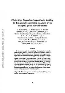
Figure 1: Illustration of the construction of a Polya tree distribution. Each of the θǫm is independently drawn from Beta(αǫm 0 , αǫm 1 ) Dirichlet process mixture model are one class. The calculation of Bayes factors for Dirichlet processbased models is discussed by Basu and Chib [2003]. Goodness of fit testing using mixtures of triangular distributions is given by McVinish et al. [2009]. An alternative form of prior, the P´ olya tree, was considered by Berger and Guglielmi [2001]. Simple conditions on the prior lead to absolutely continuous distributions. Berger and Guglielmi [2001] develops a default approach and considers its properties as a conditional frequentist method. Hanson [2006] discusses the use of Savage-Dickey density ratios to calculate Bayes factors in favour of the centering distribution (see also Branscum and Hanson [2008]). Consistency issues are discussed in general by Dass and Lee [2004] and McVinish et al. [2009]. There has been less work on testing the hypothesis that two distributions are the same. Pennell and Dunson [2008] develop a Mixture of Dependent Dirichlet Processes approach to testing changes in an ordered sequence of distributions. However, rather than using Bayes factors, a tolerance measure approach is developed. Of course, Bayesian parametric hypothesis testing where F (1) and F (2) are of known form is well developed in the Bayesian literature, see e.g. Bernardo and Smith [2000]. In the non-Bayesian literature nonparametric hypothesis testing is a mature discipline. Well known procedures include the Wilcoxon Signed-Rank test and the Kolmogorov-Smirnov test see e.g. Lehmann and Romano [2008]. Chapter 5 in Andersen et al. [1993] provides details of associated methods in survival analysis. However, none of these non-Bayesian procedures provide an explicit probabilistic measure of P (H0 |y(1,2) ) which is our interest here. We would argue that phrasing the test in a probabilistic fashion is a natural approach from which to report the evidence for H0 . The rest of the paper is as follows. In section 2 we discuss the Polya tree prior and derive the marginal probability distributions that result. In section 3 we describe our method and algorithm for calculating Pr(H0 |y(1,2) ) based on subjective priors. In section 4 we discuss an empirical Bayes procedure where the Polya Tree priors are centered on the empirical cdf of the joint data. Section 5 concludes with a brief discussion.

2

Polya tree priors

Polya trees form a class of distributions for random probability measures F on some domain Ω, Lavine [1992], Mauldin et al. [1992], Lavine [1994]. The Polya tree has a simple constructive formulation that we now describe. Consider a dyadic (binary) tree that recursively partitions Ω into disjoint measurable sets such m (m) (m) (m) = ∅ for all i 6= j. where Bi ∪ Bj that at the mth level of the tree we find Ω = ∪2j=0−1 Bj Figure 1, adapted from Ferguson [1974], illustrates such a tree up to level 2 where Ω = [0, 1). The (i+1) (i+1) (i) (i) jth junction in the tree at level i has associated set Bj and clearly Bj = (B2j , B2j+1 ) for all i, j. Conceptually we should imagine such a tree descending ad infinitum. It will be convenient in what follows to simply index the sets using base 2 subscript and drop the superscript so that, for example, B000 indicates the first set in level 3, B0011 the fourth set in level 4 and so on.

2

To define a random measure on Ω we construct random measures on the sets Bj . It is instructive to imagine a particle cascading down through the tree such that at the jth junction the probability of turning left or right is θj and (1 − θj ) respectively. In addition we consider θj to be a random variable with some appropriate distribution θj ∼ πj . The sample path of the particle down to level m will be recorded in a vector ǫm = {ǫm1 , ǫm2 , . . . , ǫmm } with elements ǫmi ∈ {0, 1}, such that ǫmi = 0 if the particle went left at level i, ǫmi = 1 if it went right. In this way Bǫm denotes which partition the particle belongs to at the mth level. Given a set of θj ’s it is clear that the probability of the particle falling into the set Bǫm is just P (Bǫm ) =

m Y (θǫi )(1−ǫii ) (1 − θǫi )ǫii ,

i=1

which is just the product of the probabilities of falling left or right at each junction that the particle passes through. In this way we have defined a random measure on the partitioning sets. The Polya tree is obtained under the following conditions: that the tree descends ad infinitum, level m → ∞, and that the θj ’are random variables with Beta distributions, θj ∼ Be(αj0 , αj1 ). To be precise, let Π denote the partition structure defined by the collection of sets Π = (B0 , B1 , B00 , . . .) and let A denote the collection of parameters that determine the Beta distribution at each junction, A = (α00 , α01 , α000 , . . .). Definition: Lavine [1992] A random probability measure F on Ω is said to have a Polya tree distribution, or a Polya tree prior, with parameters (Π, A), written, F ∼ P T (Π, A), if there exists nonnegative numbers A = (1) (1) (2) (1) (1) (2) (α0 , α1 , α00 , . . .) and random variables Θ = (θ0 , θ1 , θ00 , . . .) such that the following hold: 1. all the random variables in Θ are independent; 2. for every ǫm , θǫm ∼ Be(αǫm 0 , αǫm 1 ); 3. for every m = 1, 2, . . . and every ǫ1 , ǫ2 , . . ., F (Bǫm |Θ ) =

m Y

(θǫi )(1−ǫii ) (1 − θǫi )ǫii ,

(1)

i=1

A random probability measure F ∼ P T (Π, A) is realized by sampling the θj ’s from the Beta distributions. The set Θ is infinite dimensional as the level of the tree is infinite and hence for most practicable applications the tree is truncated to a depth m. Lavine [1994] refers to this as a “partially specified” Polya tree. It is worth noting that we will not need to make this truncation in what follows and hence our test will be fully specified with analytic expressions for the marginal likelihood. By defining Π and A the Polya tree can be centered on some chosen distribution G0 so that E[F ] = G0 where F ∼ P T (Π, A). Perhaps the simplest way to achieve this is to place the partitions in Π at the quantiles of G0 and then set αǫj 0 = αǫj 1 for all j Lavine [1992]. For Y ∈ R this leads to −1 B0 = (−∞, G−1 0 (0.5)), B1 = [G0 (0.5), ∞) and more generally at level m, −1 ∗ ∗ m m Bǫj = [G−1 0 {(j − 1)/2 }, G0 (j /2 )),

(2)

where j ∗ is the decimal representation of the binary number ǫj . It is usual to set the α’s to be constant in a level αǫm 0 = αǫm 1 = cm for some constant cm . The setting of cm governs the underlying continuity of the resulting F ’s. For example, setting cm = cm2 , c > 0, implies that F is absolutely continuous with probability 1 while cm = c/2m defines a Dirichlet process which makes F discrete with probability 1 Lavine [1992], Ferguson [1974]. We will follow the approach of Walker and Mallick [1999] and define cm = cm2 . The choice of c is left to Section 3.

2.1

Conditioning and marginal likelihood

An attractive feature of the Polya tree prior is the ease with which we can condition on data. Polya trees exhibit conjugacy since given a Polya tree prior F ∼ P T (Π, A) and a set of data y, the posterior

3

distribution on F is also a Polya tree, F |y ∼P T (Π, A∗ ) where A∗ is the set of updated parameters, A∗ = {α∗00 , α∗01 , α∗000 , . . .} with (3) α∗ǫi |y =αǫi + nǫi , where nǫi denotes the number of observations in y that lie in the partition Bǫi . The corresponding random variables θj∗ are therefore distributed a posteriori as θj∗ |y =Be(αj0 + nj0 , αj1 + nj1 )

(4)

where nj0 and nj1 are the numbers of observations falling left and right at the junction in the tree indicated by j. This conjugacy allows for a straightforward calculation of the marginal likelihood for any set of observations. A priori we see, Y nj0 (5) θj (1 − θj )nj1 Pr(y|Θ, Π, A) = j

θj |A ∼ Be(αj0 , αj1 )

where the product in (5) is over the set of all partitions, j ∈ {0, 1, 00, . . . , }, though clearly for many partitions we have nj0 = nj1 = 0. Equation (5) has the form of a product of independent BinomialBeta trials hence the marginal likelihood is, Y Γ(αj0 + αj1 ) Γ(αj0 + nj0 )Γ(αj1 + nj1 ) . (6) Pr(y|Π, A) = Γ(αj0 )Γ(αj1 ) Γ(αj0 + nj0 + αj1 + nj1 ) j where j ∈ {0, 1, 00, . . . , }. This marginal probability will form the basis of our test for H0 which we describe in the next section.

3

A procedure for subjective Bayesian nonparametric hypothesis testing

We are interested in providing a weight of evidence in favour of H0 given the observed data. From Bayes theorem, Pr(H0 |y(1,2) ) ∝Pr(y(1,2) |H0 )Pr(H0 ). (7) Recall that the null hypothesis H0 assumes y(1) and y(2) are samples from some common distribution F (1,2) with F (1,2) unknown and we specify our uncertainty in F (1,2) via a Polya tree prior, F (1,2) ∼ P T (Π, A). Under H1 , we assume y(1) ∼ F (1) , y(2) ∼ F (2) with F (1) , F (2) unknown. Again we adopt a Polya tree prior for F (1) and F (2) with the same prior parameterization as for F (1,2) so that iid

F (1) , F (2) , F (1,2) ∼ P T (Π, A)

(8)

where Π is centered on the quantiles of some a priori centering distribution (see below). Following the approach of Walker and Mallick [1999], Mallick and Walker [2003] we take common values for the αj ’s at each level as αj0 = αj1 = m2 for in α parameter at level m. The posterior odds of the two hypothesis is Pr(y(1,2) |H0 ) Pr(H0 ) Pr(H0 |y(1,2) ) = (9) Pr(H1 |y(1) ,y(2) ) Pr(y(1) ,y(2) |H1 ) Pr(H1 ) where the first term is just the ratio of marginal likelihoods, the Bayes Factor, which from (6) and conditional on our specification of Π and A is Y P (y(1,2) |H0 ) = (1) (2) P (y ,y |H1 ) j

(1)

(2)

(1)

(2)

j0

j0

j1

j1

Γ(αj0 )Γ(αj1 ) Γ(αj0 + nj0 + nj0 )Γ(αj1 + nj1 + nj1 ) × Γ(αj0 + αj1 ) Γ(αj0 + n(1) + n(2) + αj1 + n(1) + n(2) )

(10)

(1)

(1)

(2)

(2)

(1)

(1)

(2)

(2)

Γ(αj0 + nj0 + αj1 + nj1 ) Γ(αj0 + nj0 + αj1 + nj1 ) Γ(αj0 + nj0 )Γ(αj1 + nj1 ) Γ(αj0 + nj0 )Γ(αj1 + nj1 ) 4

!

(1)

(1)

where the product is over all partitions, j ∈ {0, 1, 00, . . . , }, nj0 and nj1 represent the numbers of (1) nj0

(1) nj1

are the equivalent quantities and observations in y(1) falling right and left at each junction and for y(2) . The product in (10) is defined over the infinite set of partitions. However, all terms cancel for which (1) (1) (2) (2) three of {nj0 , nj1 , nj0 , nj1 } are zero. That is, to calculate (10) for the infinite partition structure we just have to multiply terms from junctions which contain at least some samples going right and left. Hence, we only need specify Π to the quantile level where partitions contain more than one observation. Our algorithm is as follows: Algorithm 1 Bayesian nonparametric test 1. Fix the binary tree on the quantiles of some centering distribution G. 2. Set αj = m2 where m denotes the level in the tree of the corresponding junction. 3. Add the log of the contributions of terms in (10) for each junction in the tree that have non-zero numbers of observations in y(1,2) going both right and left. 4. Report Pr(H0 |y(1,2) ) as Pr(H0 |y(1,2) ) =

1 1 + exp(−LOR)

(11)

where LOR denotes the log odd ratio calculated at step 3.

3.1

Prior specification

The Bayesian procedure requires the specification of {Π, A} in the Polya tree. While there are good guidelines for setting A the setting of Π is more problem specific. Our current, default, guideline is to first standardise the joint data y(1,2) to have mean 0 and standard deviation 1 and then set the partition on the quantiles of a standard normal density, Π = Φ(·)−1 . We have found this to work well as a default in most situations, though of course the reader is encourage to set Π according to their subjective beliefs.

3.2

Characteristics (l)

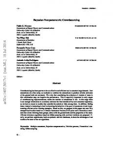
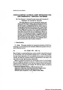
We can explore the contribution of each term in (10) as a function of njk , k ∈ {0, 1}, l ∈ {1, 2}. We can see from (10) that the overall Bayes Factor has the form of a product of Beta-Binomial tests (1) (2) at each junction in the tree to be interpreted as “do you need one θj or two, {θj , θj }, in order to model the distribution of the data going left and right at each junction”. Figure 2 shows the (2) (1) contribution from terms where nj0 = nj1 = 0, 1, . . . , n for n = 10, 100, 1000 in the first, second and third columns respectively and for α = 0.1, 10 in the first and second rows respectively. We can see that as the proportion of data going left moves away from 50% then each term starts to provide increasing evidence against the null. In Figure 2, the curvature of the log marginal likelihood ratio is changing with n; note changes in the vertical scale as n changes. In Figure 3 we look at the frequentist distribution of Pr(H1 |y) when y is generated under the null y(1) , y(2) ∼ N (0, 1) assuming a priori Pr(H1 ) = 0.5. For given sample size n, on the x-axis, we repeatedly drew 1000 data sets under the null, calculating the probability assigned to the alternative hypothesis for each set. The expected value as a function of sample size along with 90% confidence intervals is shown in Figure 3. We can see that the estimator appears to be consistent in converging to 0 as n → ∞ though we have been unable to prove this result holds for any H0 : F (1,2) .

5

Log MLR, α = 0.1

n = 10

n = 1000

50

500

0

0

0

−5

−50

−500

−10

−100

−1000

−15

Log MLR, α = 10

n = 100

5

0

0.5

1

−150

0

0.5

1

−1500

5

50

500

0

0

0

−5

−50

−500

−10

−100

−1000

−15

0

0.5 Proportion going left

1

−150

0


1

−1500

0

0.5

1

0


1

Figure 2: Shows the log marginal likelihood ratio as a function of n and α for the symmetric case (2) (1) n01 = n00 = 1, 2, . . . , n.

1

0.9

0.8

0.7

1

Pr(H | Y)

0.6

0.5

0.4

0.3

0.2

0.1

0 1 10

2

3

10

10

4

10

N

Figure 3: Shows the frequentist distribution, mean and 90% confidence intervals, for P (H1 |y) as a function of sample size, N , when samples are drawn under the null y(1) , y(2) ∼ N (0, 1) for prior Pr(H1 ) = 0.5.

6

3.3

Simulations

To examine the operating performance of the method we consider the following experiments designed to explore various canonical departures from the null. a) Mean shift: Y (1) ∼ N (0, 1), Y (2) ∼ N (θ, 1), θ = 0, . . . , 3 b) Variance shift: Y (1) ∼ N (0, 1), Y (2) ∼ N (0, θ2 ), θ = 1, . . . , 3 c) Mixture: Y (1) ∼ N (0, 1), Y (2) ∼ 21 N (θ, 1) + 21 N (−θ, 1), θ = 0, . . . , 3 d) Tails: Y (1) ∼ N (0, 1), Y (2) ∼ t(θ−1 ), θ = 10−3 , . . . , 10 e) Skew: Y (1) ∼ N (0, 1), Y (2) ∼ SN (0, 1, θ), θ = 1, . . . , 10 f ) Outlier: Y (1) ∼ N (0, 1), Y (2) ∼ (1 − θ)N (0, 1) + θN (0, 20), θ = 0, . . . , 1 g) Lognormal mean shift: log Y (1) ∼ N (0, 1), log Y (2) ∼ N (θ, 1), θ = 0, . . . , 3 h) Lognormal variance shift: log Y (1) ∼ N (0, 1), log Y (2) ∼ N (0, θ2 ), θ = 1, . . . , 3 where SN (0, 1, λ) is the skew normal distribution of skewness parameter λ. The default mean dis(1,2) tribution F0 = N (0, 1) was used in the Polya tree to construct the partition Π and α = m2 . Data are standardized. Comparisons are performed with n0 = n1 = 50 against the two-sample Kolmogorov-Smirnov and Wilcoxon rank test. To compare the models we explore the “power to detect the alternative”. As a test statistic for the Bayesian model we simulate data under the null and then take the empirical 0.95 quantile of the distribution of Bayes Factors as a threshold to declare H1 . This is known as “the Bayes, non-Bayes compromise” by Good [1992]. Results are reported in Figure 4. As a general rule we can see that the KS test is more sensitive to changes in central location while the Bayes test is more sensitive to changes to tails or higher moments. We also see that the subjective Bayes test appears to be inconsistent in some circumstances and fails to detect changes to the degrees of freedom of a t-density to a normal. One clear advantage of the Bayesian model is that it provides an explicit measure of P (H1 |y). The expectation of Pr(H1 |y) arising from the simulations in Figure 4, along with 90% frequentist confidence intervals, derived from 100 repeated simulations, is shown in Figure 5. Again, we observe the inconsistency of the subjective Bayes test to detect tail changes between a normal and t-distribution; with all other tests showing intuitive performance. We investigated a more diffuse distribution for the centering distribution of the Polya Tree Π = [G(1,2) ]−1 , such as G(1,2) ≡ N (0, 2) and G(1,2) ≡ t(2) but the behavior still persists. The dyadic partition structure of the Polya Tree allows us to breakdown the contribution to the Bayes Factor by levels. That is, we can explore the contribution, in the log of equation (10), by level. This is shown in Figure 6 as boxplots of the distribution of log BF statistics across the levels for the simulations generated for Figure 4. This is a strength of the Polya tree test in that it provides a qualitative and quantitative decomposition of the contribution to the evidence against the null from differing levels of the tree. For example, we observe that shifts in central location are, unsurprisingly, detected at the top most level of the tree, while changes to the tails or variances are detected further down in the quantiles or below. This provides the statistician with a useful gauge on where signal against the null is coming from. We next explore sensitivity to the prior parameters α = cm2 by changing the constant such that α = 10m2 . Figures 7 and 8 show the corresponding results analogous to Figure 4 and Figure 6 with α = m2 . Increasing the constant places greater contribution to the higher levels of the tree and hence we find that setting c = 10 improves the precision to detect a shift in central location at the expense to sensitivity to lower quantiles such as tail and higher moment detection.

4

An empirical Bayes procedure

The Bayesian procedure above requires the subjective specification of the partition structure Π. This subjective setting may make some users uneasy regarding the sensitivity to specification. Moreover, we have seen for certain tests under H1 the subjective test performs poorly. In this section we explore 7

an empirical procedure, akin to empirical Bayes, whereby the partition Π is centered on the data via h i−1 ˆ = Fˆ (1,2) . This is akin to an empirical Bayes procedure with the empirical cdf of the joint data Π

ˆ to the marginal MAP estimate. The empirical cdf maximises a flat prior over π(Π) and the setting Π the marginal likelihood when using symmetric Be(αj , αj ) priors, as a priori we expect to see equal numbers of observations going left or right at any junction in the tree. This provides a default setting for the partition. ˆ be the partition constructed with the quantiles of the empirical distribution Fˆ (1,2) of y (1,2) . Let Π Under H0 , there are now no free parameters and only one degree of freedom in the random variables (2) (2) (1) (1) {nj0 , nj1 , nj0 , nj1 } as conditional on the partition centered on the empirical cdf of the joint, once one of variables has been specified the others are then known. We consider, arbitrarily, the marginal (1) distribution of {nj0 } which is now a product of hypergeometric distributions (we only consider levels (12)

where nj

> 1) (1)

(1) ˆ A) ∝ P r({nj0 }|H0 , Π,

nj (1) nj0

Y

!

Y

!

(12)

(12)

nj (12) nj0

j

=

(1)

(12)

nj − nj (1) (12) nj0 − nj0 !

(1)

(12)

HypGeo(nj ; nj

(1)

(12)

, nj , nj0 )

(13)

j

(12)

(12)

(1)

if max(0, nj0 + nj − nj

(1)

) ≤ nj

(12)

(1)

≤ min(nj , nj0 ), 0 otherwise. (1)

Under H1 , the marginal distribution of {nj0 } is a product of the conditional distribution of independent binomial variates, conditional on their sum, (1)

ˆ A) ∝ Pr({nj0 }|H1 , Π, (12)

(1)

(12)

if max(0, nj0 + nj − nj

(12)

(1)

g(nj0 ; nj

(1)

) ≤ nj

(1)

(12)

(1)

(1)

(2)

(1)

(1)

(1)

(12)

, nj , nj0 , θj , θj ) = Bin(nj0 ; nj , θj ) × . . . (12)

Bin(nj0 − nj0 ; nj and

(14)

≤ min(nj , nj0 ), 0 otherwise, and where (12)

(1)

(12) (1) (2) (1) (12) Y g(n(1) , nj , nj0 , θj , θj ) j0 ; nj P (12) (1) (2) (1) (12) , nj , nj0 , θj , θj ) j x g(x; nj

(1)

(2)

− n j , θj )

(2)

(1)

θj |A ∼ Be(αj0 , αj1 )

θj |A ∼ Be(αj0 , αj1 ) (1)

Now, consider the odds ωj =

θj

(2)

θj

and let (1)

(12)

(1)

W (nj0 ; nj

(12)

(1)

(12)

(1)

(2)

g(nj0 ; nj , nj , nj0 , θj , θj ) (12) (1) , nj , nj0 , ωj ) = P . (12) (1) (2) (1) (12) , nj , nj0 , θj , θj ) x g(x; nj

Then it can been seen that W (x; N, m, n, ω) is the Wallenius noncentral hypergeometric distribution Wallenius [1963], Johnson et al. [2005] whose pdf is

m x

N −m n−x

Z

1

(1 − tω/D )x (1 − t1/D )n−x dt

0

where D = ω(m − x) + (N − m − n + x). Note there are C++ and R routines to evaluate the pdf 1 . Wallenius noncentral hypergeometric distribution models a biased urn sampling scheme whereby 1 See references there http://en.wikipedia.org/wiki/Wallenius‘ noncentral hypergeometric distribution

8

there is a different likelihood of drawing one type of ball over another at each draw. The Bayes factor is now given by (12) (1) (12) (1) Y HypGeo(nj0 ; nj , nj , nj0 ) (15) BF = R∞ (12) (1) (12) (1) , nj , nj0 , ωj )p(ωj )dωj j 0 W (nj0 ; nj

where the marginal likelihood in the denominator can be evaluated using importance sampling or one-dimensional quadrature. The empirical Bayes two-sample test can then be given as: Algorithm 2 Empirical Bayes nonparametric test 1. Fix the binary tree on the quantiles of the empirical distribution Fˆ (1,2) . 2. Set αj = m2 where m denotes the level in the tree of the corresponding junction. 3. Add the log of the contributions of terms in (15), evaluated using importance sampling or quadrature, for each junction in the tree that have non-zero numbers of observations in y(1,2) going both right and left. 4. Report Pr(H0 |y(1,2) ) as Pr(H0 |y(1,2) ) =

1 1 + exp(−LOR)

(16)

where LOR denotes the log odd ratio calculated at step 3. We repeated the simulations from Section 3.3 with α = m2 . The corresponding results are shown in Figures 9, 10, 11. We observe similar behaviour to the subjective test but importantly we see that the problem in detecting the difference between normal and t-distribution is corrected. Moreover, no standardisation of the data is required for this test.

5

Conclusions

We have described a Bayesian nonparametric hypothesis test for real valued data which provides an explicit measure of Pr(H0 |y(1,2) ). The test is based on a fully specified Polya Tree prior for which we are able to derive an explicit form for the Bayes Factor. The choice of the partition is quite crucial for the subjective Bayes test. This is a well known phenomena of Polya Tree priors and some interesting directions to mitigate its effects can be found in Hanson and Johnson [2002], Paddock et al. [2003], Hanson [2006]. To this aim we also provided an automated empirical Bayes procedure which centres the partition on the empirical cdf of the joint data which was seen to rectify problems in the subjective Bayes test.

Acknowledgements This research was partly supported by the Oxford-Man Institute through a visit by the second author to the OMI.

References P.K. Andersen, O. Borgan, R.D. Gill, and N. Keiding. Statistical models based on counting processes. Springer Series in Statistics, 1993. S. Basu and S. Chib. Marginal likelihood and bayes factors for dirichlet process mixture models. Journal of the American Statistical Association, 98:224–235, 2003. J.O. Berger and A. Guglielmi. Testing of a parametric model versus nonparametric alternatives. Journal of the American Statistical Association, 96:174–184, 2001. 9

J.M. Bernardo and A.F.M. Smith. Bayesian theory. Chichester: John Wiley, 2000. A. J. Branscum and T. J. Hanson. Bayesian nonparametric meta-analysis using polya tree mixture models. Biometrics, 64:825–833, 2008. C. Carota and G. Parmigiani. On Bayes factors for nonparametric alternatives. In J. M. Bernardo, J. O. Berger, A. P. Dawid, and A. F. M. Smith, editors, Bayesian Statistics 5, pages 508–511, London, 1996. Oxford University Press. S. C. Dass and J. Lee. A note on the consistency of bayes factors for testing point null versus nonparametric alternatives. Journal of Statistical Planning and Inference, 119:143–152, 2004. T.S. Ferguson. Prior distributions on spaces of probability measures. The Annals of Statistics, 2: 615–629, 1974. J. P. Florens, J. F. Richard, and J. M. Rolin. Bayesian encompassing specification tests of a parametric model against a nonparametric alternative. Technical Report 96.08, Institut de Statistique, Universit´e Catholique de Louvain, 1996. I.J. Good. The Bayes/non-Bayes compromise: a brief review. Journal of the American Statistical Association, 87:597–606, 1992. T. Hanson and W. O. Johnson. Modeling regression error with a mixture of Polya trees. Journal of the American Statistical Association, 97:1020–1033, 2002. T. E. Hanson. Inference for mixtures of finite Polya tree models. Journal of the American Statistical Association, 101:1548–1565, 2006. N.L. Johnson, A.W. Kemp, and S. Kotz. Univariate discrete distributions. John Wiley. &. Sons, 2005. M. Lavine. Some aspects of Polya tree distributions for statistical modelling. The Annals of Statistics, 20:1222–1235, 1992. M. Lavine. More aspects of Polya tree distributions for statistical modelling. The Annals of Statistics, 22:1161–1176, 1994. E.L. Lehmann and J.P. Romano. Testing Statistical Hypotheses. Springer, 2008. B.K. Mallick and S. Walker. A Bayesian semiparametric transformation model incorporating frailties. Journal of Statistical Planning and Inference, 112:159–174, 2003. R.D. Mauldin, W.D. Sudderth, and S.C. Williams. Polya trees and random distributions. The Annals of Statistics, 20:1203–1221, 1992. R. McVinish, J. Rousseau, and K. Mengersen. Bayesian goodness of fit testing with mixtures of triangular distributions. Scandivavian Journal of Statistics, 36:337–354, 2009. S. M. Paddock, F. Ruggeri, M. Lavine, and M. West. Randomized Polya tree models for nonparametric Bayesian inference. Statistica Sinica, 13:443–460, 2003. M. L. Pennell and D. B. Dunson. Nonparametric Bayes testing of changes in a response distribution with an ordinal predictor. Biometrics, 64:413–423, 2008. S. Walker and B.K. Mallick. A Bayesian semiparametric accelerated failure time model. Biometrics, 55:477–483, 1999. K.T. Wallenius. Biased sampling: the non-central hypergeometric probability distribution. PhD thesis, Stanford University, 1963.

10

mean

var 1

1

0.9

0.9

0.8

0.8

0.8

0.7

0.7 Polya Tree Kolmogorov−Smirnov Wilcoxon

0.5

0.5

0.4

0.4

0.4

0.3

0.3

0.3

0.2

0.2

0.2

0.1

0.1

0

0

0.2

0.4

0.6

0.8

1 theta

1.2

1.4

1.6

1.8

0

2

0.1

1

1.5

(a) Gaussian: mean

2

2.5

3 sigma

3.5

4

4.5

0

5

1

0.9

0.8

0.8

0.8

0.7


0.5

0.4

0.4

0.3

0.3

0.3

0.2

0.2

0.2

0.1

0.1

5 sigma

6

7

8

9

0

10

1.4

1.6

1.8

2

0.9

1

Polya Tree Kolmogorov−Smirnov Wilcoxon

0.1

0

0.5

(d) Gaussian: tail

1

1.5

2

2.5 theta

3

3.5

4

(e) Gaussian: skewness

lognorm ean

4.5

5

0

0

0.1

0.2

0.3

0.4

0.5 theta

0.6

0.7

0.8

(f) Gaussia: outlier

lognorm ar

m

v

1

1

0.9

0.9

0.8

0.8

0.7



0.6 Power

0.6

0.5

0.5

0.4

0.4

0.3

0.3

0.2

0.2

0.1

0

1.2

0.5

0.4

4

1 theta

0.6 Power

0.5

3

0.8


0.6 Power

0.6

2

0.6

outlier

1

0.9

1

0.4

(c) Gaussian: mixture

1

0

0.2

skew

0.9

0

0

(b) Gaussian: variance

tail

Power

0.6 Power

0.5



0.6 Power

Power

0.6

Power

mixture

1

0.9

0.1

0

0.2

0.4

0.6

0.8

1 theta

1.2

1.4

1.6

(g) lognormal: mean

1.8

2

0

1

1.5

2

2.5

3 sigma

3.5

4

4.5

5

(h) lognormal: variance

Figure 4: Power of Bayes Polya Tree prior test with αj = m2 tested on simulations from Section 3.2 with Gaussian distribution with varying (a) mean (b) variance (c) Mixture (d) tails (e) skewness (f) outlier. Log-normal distribution with varying (g) mean (h) variance. The x-axis measures the value of θ, the parameter in the alternative given in Section 3.2. Legend: Kolmogorov-Smirnov test (red dashed), Wilcoxon (red dot-dashed), Bayesian nonparametric test (solid blue).

11

var

0.8

0.8

0.8

0.7

0.7

0.7

0.6

0.6

0.6

0.5

Pr(H1 | Y)

1

0.9

0.5

0.4

0.4

0.3

0.3

0.3

0.2

0.2

0.2

0.1

0.1

0

0.2

0.4

0.6

0.8

1 theta

1.2

1.4

1.6

1.8

0

2

0.1

1

1.5

(a) Gaussian: mean

2.5

3 sigma

3.5

4

4.5

0

5

1

0.9

0.8

0.8

0.8

0.7

0.7

0.7

0.6

0.6

0.6

0.5

Pr(H1 | Y)

1

0.9

0.5

0.4

0.4

0.3

0.3

0.3

0.2

0.2

0.2

0.1

0.1

2

3

4

5 sigma

6

7

8

9

0

10

0.8

1 theta

1.2

1.4

1.6

1.8

2

0.9

1

0.1

0

0.5

(d) Gaussian: tail

1

1.5

2

2.5 theta

3

3.5

4


lognorm ean

4.5

5

0

0

0.1

0.2

0.3

0.4

0.5 theta

0.6

0.7

0.8

(f) Gaussian: outlier

lognorm ar

m

v

1

0.9

0.8

0.8

0.7

0.7

0.6

0.6 Pr(H | Y)

1

0.9

1

0.5

0.5

0.4

0.4

0.3

0.3

0.2

0.2

0.1

0

0.6

0.5

0.4

1

0.4

outlier

1

0

0.2


0.9

0

0

skew

Pr(H1 | Y)

Pr(H1 | Y)

2


tail

1

0.5

0.4

0

Pr(H | Y)

mixture

1

0.9

Pr(H1 | Y)

1

Pr(H | Y)

mean 1

0.9

0.1

0

0.2

0.4

0.6

0.8

1 theta

1.2

1.4

1.6

(g) lognormal: mean

1.8

2

0

1

1.5

2

2.5

3 sigma

3.5

4

4.5

5


Figure 5: Expected probability of H1 , with 90% frequentist confidence intervals by repeatedly applying the Bayes Polya Tree prior test with αj = m2 for tests show in Figure 4. x-axis records the value of θ the parameter of the alternative on same scale as Figure 4.

12

mean, θ = 1

var, σ = 3

mixture, θ = 1

40 20 20

35

25

20

15

10

Contribution to Log Bayes Factor



30 15

10

5

15

10

5

5 0

0 0 1

2

3

4

5

6

7

8

9

10

1

2

3

4

5

Level

6

7

8

9

10

1

2

3

4

5

Level

(a) Gaussian: mean


7

8

9

10

9

10


skew, θ = 2.5

tail, σ = 4.5

6 Level

outlier, θ = 0.5

0

16 −1

20 14

−4 −5 −6 −7

12


−3



−2

10

8

6

4

15

10

5

−8

2 −9

0

0

−10

−2 1

2

3

4

5

6

7

8

9

1

10

2

3

4

5

6

7

8

Level

Level

(d) Gaussian: tail

10

1

2

3

4

5

6

7

8

Level


lognorm ean, θ = 1

9


lognorm ar, σ = 3

m

v

45 25

40

35 Contribution to Log Bayes Factor


20 30

25

20

15

10

15

10

5

5 0 0 1

2

3

4

5

6

7

8

Level

(g) lognormal: mean

9

10

1

2

3

4

5

6

7

8

9

10

Level


Figure 6: Contribution to Bayes Factors from different levels of the Polya Tree under the alternative. Gaussian distribution with varying (a) mean (b) variance (c) Mixture (d) tails (e) skewness (f) outlier; Log-normal distribution with varying (g) mean (h) variance, from Section 3.2. Parameters of H1 were set to the mid-points of the x-axis in Figure 4

13

mean

var 1

1

0.9

0.9

0.8

0.8

0.8

0.7


0.5

0.5

0.4

0.4

0.4

0.3

0.3

0.3

0.2

0.2

0.2

0.1

0.1

0

0

0.2

0.4

0.6

0.8

1 theta

1.2

1.4

1.6

1.8

0

2

0.1

1

1.5

(a) Gaussian: mean

2

2.5

3 sigma

3.5

4

4.5

0

5

0.9

0.9

0.9

0.8

0.8

0.8

0.7


0.5

0.4

0.4

0.3

0.3

0.3

0.2

0.2

0.2

0.1

0.1

5 sigma

6

7

8

9

0

10

1.4

1.6

1.8

2

0.9

1


0.1

0

0.5

(d) Gaussian: tail

1

1.5

2

2.5 theta

3

3.5

4


lognormmean

4.5

5

0

0

0.1

0.2

0.3

0.4

0.5 theta

0.6

0.7

0.8


lognormvar

1

1

0.9

0.9

0.8

0.8

0.7



0.6 Power

0.6

0.5

0.5

0.4

0.4

0.3

0.3

0.2

0.2

0.1

0

1.2

0.5

0.4

4

1 theta

0.6 Power

0.5

3

0.8


0.6 Power

0.6

2

0.6

outlier 1

1

0.4


1

0

0.2

skew

1

0

0


tail

Power

0.6 Power

0.5



0.6 Power

Power

0.6

Power

mixture

1

0.9

0.1

0

0.2

0.4

0.6

0.8

1 theta

1.2

1.4

1.6

(g) lognormal: mean

1.8

2

0

1

1.5

2

2.5

3 sigma

3.5

4

4.5

5


Figure 7: Same as Figure 4 but now with αj = 10m2 . Gaussian distribution with varying (a) mean (b) variance (c) Mixture (d) tails (e) skewness (f) outlier. Log-normal distribution with varying (g) mean (h) variance. Legend: Kolmogorov-Smirnov test (red dashed), Wilcoxon (red dashed-dot), Bayesian nonparametric test (solid blue)

14

var, σ = 3

mean, θ = 1

mixture, θ = 1

30

6 6 25

5

15

10




5

20

4

3

2

4

3

2

1

1 5

0

0

0 1

2

3

4

5

6

7

8

9

1

10

2

3

4

5

6

7

8

9

10

1

2

3

4

5

Level

Level

(a) Gaussian: mean


7

8

9

10

9

10

(c) Gaussian: mixture outlier, θ = 0.5

skew, θ = 2.5

tail, σ = 4.5

6 Level

7 12

−1

6 −2



−4

−5

−6

−7

−8


10 −3

8

6

4

5

4

3

2

1

2

−9

0 0

−10 1

2

3

4

5

6

7

8

9

1

10

2

3

4

5

6

7

8

(d) Gaussian: tail


lognorm ean, θ = 1

10

1

2

3

4

5

6

7

8

Level

Level

Level

9


lognorm ar, σ = 3

m

v

7 30 6 25 Contribution to Log Bayes Factor


5

20

15

10

4

3

2

1 5 0 0

−1 1

2

3

4

5

6

7

8

Level

(g) lognormal: mean

9

10

1

2

3

4

5

6

7

8

9

10

Level


Figure 8: Contributions to BFs using αj = 10m2 . Gaussian distribution with varying (a) mean (b) variance (c) Mixture (d) tails (e) skewness. Log-normal distribution with varying (f) mean (g) variance. Legend: Kolmogorov-Smirnov test versus Bayesian nonparametric test. Parameters of H1 were set to the mid-points of the x-axis in Figure 4.

15

mean

var 1

1

0.9

0.9

0.8

0.8

0.8

0.7


0.5

0.5

0.4

0.4

0.4

0.3

0.3

0.3

0.2

0.2

0.2

0.1

0.1

0

0

0.2

0.4

0.6

0.8

1 theta

1.2

1.4

1.6

1.8

0

2

0.1

1

1.5

(a) Gaussian: mean

2

2.5

3 sigma

3.5

4

4.5

0

5

0.9

0.9

0.9

0.8

0.8

0.8

0.7


0.5

0.4

0.4

0.3

0.3

0.3

0.2

0.2

0.2

0.1

0.1

5 sigma

6

7

8

9

0

10

1.4

1.6

1.8

2

0.9

1


0.1

0

0.5

(d) Gaussian: tail

1

1.5

2

2.5 theta

3

3.5

4


lognormmean

4.5

5

0

0

0.1

0.2

0.3

0.4

0.5 theta

0.6

0.7

0.8


lognormvar

1

1

0.9

0.9

0.8

0.8

0.7



0.6 Power

0.6

0.5

0.5

0.4

0.4

0.3

0.3

0.2

0.2

0.1

0

1.2

0.5

0.4

4

1 theta

0.6 Power

0.5

3

0.8


0.6 Power

0.6

2

0.6

outlier 1

1

0.4


1

0

0.2

skew

1

0

0


tail

Power

0.6 Power

0.5



0.6 Power

Power

0.6

Power

mixture

1

0.9

0.1

0

0.2

0.4

0.6

0.8

1 theta

1.2

1.4

1.6

(g) lognormal: mean

1.8

2

0

1

1.5

2

2.5

3 sigma

3.5

4

4.5

5


Figure 9: Empirical Bayes Test using αj = m2 . Power to detect Gaussian distribution with varying (a) mean (b) variance (c) Mixture (d) tails (e) skewness (f) outlier and Log-normal distribution with varying (g) mean (h) variance; as in Section 3.2. Legend: Kolmogorov-Smirnov test (red dashed), Wilcoxon (red dot-dashed), Bayesian nonparametric test (solid blue).

16

var

0.8

0.8

0.8

0.7

0.7

0.7

0.6

0.6

0.6

0.5

Pr(H1 | Y)

1

0.9

0.5

0.4

0.4

0.3

0.3

0.3

0.2

0.2

0.2

0.1

0.1

0

0.2

0.4

0.6

0.8

1 theta

1.2

1.4

1.6

1.8

0

2

0.1

1

1.5

(a) Gaussian: mean

2.5

3 sigma

3.5

4

4.5

0

5

0.9

0.8

0.8

0.8

0.7

0.7

0.7

0.6

0.6

0.6

0.5

Pr(H1 | Y)

0.9

0.5

0.4

0.4

0.3

0.3

0.3

0.2

0.2

0.2

0.1

0.1

2

3

4

5 sigma

6

7

8

9

0

10

0.8

1 theta

1.2

1.4

1.6

1.8

2

0.9

1

0.1

0

0.5

(d) Gaussian: tail

1

1.5

2

2.5 theta

3

3.5

4


lognormmean

4.5

5

0

0

0.1

0.2

0.3

0.4

0.5 theta

0.6

0.7

0.8


lognormvar 1

0.9

0.8

0.8

0.7

0.7

0.6

0.6 Pr(H | Y)

1

0.9

1

0.5

0.5

0.4

0.4

0.3

0.3

0.2

0.2

0.1

0

0.6

0.5

0.4

1

0.4

outlier

1

0.9

0

0.2

(c) Gaussian: mixture 1

0

0

skew 1

Pr(H1 | Y)

Pr(H1 | Y)

2


tail

1

0.5

0.4

0

Pr(H | Y)

mixture

1

0.9

Pr(H1 | Y)

1

Pr(H | Y)

mean 1

0.9

0.1

0

0.2

0.4

0.6

0.8

1 theta

1.2

1.4

1.6

(g) lognormal: mean

1.8

2

0

1

1.5

2

2.5

3 sigma

3.5

4

4.5

5


Figure 10: Expected probability of empirical Bayes test for H1 , with 90% confidence intervals by repeatedly applying the Bayes Polya Tree prior test with αj = m2 on Gaussian distribution with varying (a) mean (b) variance (c) Mixture (d) tails (e) skewness (f) outlier and log-normal distribution with varying (g) mean (h) variance, as in Section 3.2.

17

var, σ = 3

mean, θ = 1 35

mixture, θ = 1

25

30

20

20

15

10




20 25

15

10

5

15

10

5

5 0

0 0 1

2

3

4

5

6

7

8

9

10

1

2

3

4

5

Level

6

7

8

9

10

1

2

3

4

5

Level

(a) Gaussian: mean


7

8

9

10

9

10


skew, θ = 2.5

tail, σ = 4.5

6 Level

outlier, θ = 0.5

14 20

20

15

10

5




12

10

8

6

4

15

10

5

2

0

0

0

−2 1

2

3

4

5

6

7

8

9

10

1

2

3

4

5

Level

6

7

8

Level

(d) Gaussian: tail

10

1

2

3

4

5

6

7

8

Level


lognorm ean, θ = 1

9


lognorm ar, σ = 3

m

v

25

35

30 Contribution to Log Bayes Factor


20 25

20

15

10

15

10

5 5 0 0 1

2

3

4

5

6

7

8

Level

(g) lognormal: mean

9

10

1

2

3

4

5

6

7

8

9

10

Level


Figure 11: Contribution to the Bayes Factor for differing levels of the empirical Polya Tree prior for Gaussian distribution with varying (a) mean (b) variance (c) Mixture (d) tails (e) skewness (f) outlier. Log-normal distribution with varying (g) mean (h) variance.

18