NONPARAMETRIC LEARNING CAPABILITIES OF FUZZY SYSTEMS
Author: Manuel Landajo Statistics and Econometrics Unit Department of Applied Economics University of Oviedo Avenida del Cristo s/nº 33006 Oviedo Spain
e-mail:
[email protected] Fax: +34-985-105050 Telephone: +34-985-105055
1
Nonparametric Learning Capabilities of Fuzzy Systems Manuel Landajo University of Oviedo
Abstract—Nonparametric estimation capabilities of fuzzy systems in stochastic environments are analyzed in this paper. By using ideas from sieve estimation, increasing sequences of fuzzy rule-based systems, capable of consistently estimating regression surfaces in different settings, are constructed. Results include least squares learning of a mapping perturbed by additive random noise in a static-regression context and least squares learning of a regression surface from data generated by a bounded stationary ergodic random process. L1 estimation is also studied, and the consistency of fuzzy rule-based sieve estimators for the L1 optimal regression surface is shown, thus giving additional theoretical support to the robust filtering capabilities of fuzzy systems and their adequacy for modeling, prediction and control of systems affected by impulsive noise. Index terms—fuzzy systems, nonparametric sieve estimation, consistency, least squares learning, robust learning
2 I.
INTRODUCTION AND MOTIVE
In a series of recent papers (Kosko [16], Wang and Mendel [31], Nguyen et al. [24], Mao et al. [23], Zeng and Singh [39-40], Kreinovich et al. [18], Landajo et al. [22], among others), fuzzy rule-based systems have been shown to be universal approximators in a wide variety of function spaces with practical relevance. Mathematical content is thus given to one of the aspects of flexibility or model-freedom of fuzzy models. As is well known, fuzzy systems (FSs) possess at least one other additional source of flexibility: they can be constructed both from expert information supplied by the modeler and from statistical data by using adequate neural and/or statistical training devices. In many practical applications, both sources of knowledge are combined in order to efficiently construct an FS with optimal (or, at least, sufficient) performance. Since fuzzy modelers became aware of the advantages of automatic or semi-automatic model-building procedures, a vast array of literature has appeared on the subject. A number of statistical learning mechanisms –including, e.g., batch and on-line algorithms for rule-tuning, cross-validation-based techniques for model selection and evaluation of model performance− have been adapted, and often specifically designed, to enhance the performance of FSs (e.g., Takagi and Sugeno [29], Sugeno and Tanaka [28], Kosko [14-15], Wang [32], Jang [12], and many others, the list is far from complete). A survey of the above literature suggests that the fuzzy or neuro-fuzzy community has adopted an essentially pragmatic view as to the use of statistical ideas and methods, often applying them on an ad hoc basis, with practically no reference to any probabilistic framework underlying such methods and with a limited use of the statistical inference apparatus. A few exceptions are, e.g., works by Kosko [15, 17], Watanabe and Imaizumi [33], and Wang [32]. In all these cases, fuzzy systems are explicitly viewed as approximators to regression surfaces or to other deterministic characteristics of probability distributions, and formal probabilistic and statistical inference analyses are conducted in order to study the behavior of fuzzy systems in random settings. In spite of the relative meagerness of such kinds of analyses, there are important reasons for a formal study of the statistical behavior of fuzzy systems, or equivalently,
3 to analyze their performance in stochastic environments. First, in practical applications, fuzzy rule-based models are required to satisfactorily perform tasks such as modeling, control and forecasting of systems affected by random noise. In such cases, noise must be filtered out in order for fuzzy models to perform successfully. Since, as noted by Wang ([32], Chapter 7), the presence of random noise is the rule rather than the exception, FSs should also possess good statistical properties in addition to their fuzzy logic support. Secondly, model freedom has been advocated as an important advantage of fuzzy systems that enables them to be used as flexible approximators for arbitrary mappings, or more generally, as nonparametric estimators for regression surfaces (see Kosko [16]). Thus, nonparametric learning results are a natural complement to the above-mentioned universal approximation theorems: while the latter are concerned with what FSs can do, the former would try to answer the question of how they can do it, i.e., how to learn from experience. Plainly stated, universal approximation theorems (which often are simply existence theorems) may become useless if not complemented with results showing the way to construct models from a limited amount of information obtained from the real system under study. Finally, statistical analyses of the performance of FSs in random contexts enable us to directly compare them to standard modeling paradigms such as linear state space models, as well as to neural networks, series estimators and other model-free methodologies. Empirical comparisons such as those in Kosko [15, Chapters 9-11] may thus find a good complement in analytical results. Due to the above-mentioned reasons, and regardless of the various epistemological positions on fuzzy sets and their semantics, a formal answer to the question of what fuzzy rule-based systems do in stochastic environments seems of considerable interest. In this paper, we purport to direct the attention of researchers to that point and to provide some additional insight on the subject. Since the matter is obviously very broad, we will restrict ourselves to formalizing only some of the ideas about the role of fuzzy systems as regression tools. For this, we will take advantage of a number of important results obtained in recent years in the closely related field of artificial neural networks (ANNs). At least in the last decade, the ANN community has become increasingly prone to use the toolkit of mathematical statistics to better understand many aspects of learning processes in neural models. The interface between neural networks and statistics has shown to be rather fruitful, giving birth to a rich resource of literature on
4 statistical properties regarding neural models and their learning mechanisms (see, e.g., White [34-36], Kuan and White [19], Geman et al. [9]). All these −and many other− contributions have provided a natural complement to the now well-known universal approximation properties of neural nets and have solidly established them as flexible regression tools. Analogous to the ANN case, in the context of fuzzy (or neuro-fuzzy) systems, the problem of learning from statistical data may also be seen in terms of nonparametric estimation. In principle, we can use the flexibility of FSs (i.e., their universal approximation
capabilities)
in
order
to
approximate
certain
non-stochastic
characteristics of the modeled system. Then, in order to solve the learning problem, adequate estimation mechanisms must be implemented and their convergence to the relevant characteristics of the real system must be assured. This is precisely the main goal of this paper. Our scheme should also be encompassing enough to include another relevant aspect of fuzzy modeling, i.e., the above-mentioned combination of statistical and expert information (Zadeh [38]). As we shall see, expert information plays an important role in our results, since in fact it directs (i.e., usefully constrains) the whole learning process, which in this way turns out to be simpler than the purely black-box learning of ANNs. The importance of this difference among the purely neural and the fuzzy (or neuro-fuzzy) paradigms has been greatly stressed in literature (see, e.g., Nguyen et al. [24], Kim and Mendel [13]). In this paper, we adapt some of the results from the statistical literature on neural networks in order to show that a mainstream class of fuzzy models equipped with a standard training mechanism provides a consistent nonparametric estimation device, capable of asymptotically learning arbitrary regression surfaces. The structure of the paper is as follows: Section II reviews the basic estimation setting and the ideas of sieve estimation, and explores its connection to neuro-fuzzy (and to general) rule-based modeling. Section III contains several nonparametric results that establish the consistency of our fuzzy rule-based sieve estimators for arbitrary regression surfaces, both under i.i.d. and (bounded) stationary ergodic data-generating processes, and for several learning criteria (least squares and minimum L1 distance). Section IV contains
5 the conclusions and further research lines. Mathematical proofs are included in the Appendix.
II.
LEARNING IN FUZZY SYSTEMS AND MODEL-FREE STATISTICAL ESTIMATION Briefly, our problem may be summarized in the following terms: the researcher is
interested in approximating a certain (non-stochastic) characteristic of a real system, namely an unknown regression surface θ* , which is a point in a certain function space Θ . Since in most real world problems the probability laws associated with the modeled system are unknown, the researcher must try to learn the θ* based on the partial information at his/her disposal. This may come from two sources: 1) contour information on the modeled system, and 2) statistical data, i.e., a finite (random or at least stochastic-like) sample of input-output pairs, obtained from observation or experimentation on the modeled system. At this point, the common (fuzzy) modeling practice proceeds as follows: the modeler’s aim is to use the above information in order to construct an adequate (fuzzy) model, the performance of which must be optimal in terms of a properly chosen cost function. As is well known, least squares fitting is the leading choice, but any other quantitative criterion that grants a well-defined optimization scheme may be acceptable. An important point in the above framework is that the modeler’s goal is not that of memorizing the sample information, but rather that of constructing fuzzy systems that behave optimally for the whole population. Such a requirement –which evidently amounts to the use of learning mechanisms with good generalization capabilities– is common to both neural and fuzzy models and, indeed to every statistical estimation scheme. The arguments provided by H. White [35], who presents a detailed discussion on the relevance of the statistical inference viewpoints to the neural networks paradigm, may be directly applied to the case of fuzzy systems when used to perform in stochastic environments. For the sake of brevity, we omit the details, which can be found in the mentioned (and related) papers.
6 A. Sieve Estimation The method of sieves, proposed by U. Grenander [11] and originally devised to bypass several drawbacks of standard maximum likehood estimation in infinite dimensional parametric spaces (see [11], and Geman and Wang [10]), has received increasing attention in recent years in statistical literature. It provides a general-purpose scheme that is useful for deriving well-behaved estimators in very general settings. In fact, many standard non-parametric estimation schemes −including neural networks (White [36]) and series estimators based on trigonometric functions, splines and wavelets (see, e.g., Elbadawi et al. [5], Andrews [1], Chen and Shen [2])− may be seen as particular classes of sieve extremum estimators. In sieve estimation, the object to be learned is a point θ* lying in a set Θ (generally an abstract space endowed with a certain metric). The method of sieves replaces an estimation process which requires optimization to be carried out on the entire parameter space Θ by a sequence of well-defined estimation problems that have the same limit. In essence, a sieve
{Θ m }
is an increasing sequence of parametric models whose
complexity is indexed by m . This sequence is generally required to be dense in Θ , and thus sieve estimation always relies on the availability of appropriate classes of universal approximators in Θ . Another basic point is usually that of permitting m to increase slowly enough with sample size n , in order to asymptotically avoid both overfitting and underfitting, and to obtain convergence to θ* . B. Fuzzy Rule-Based Sieves The ideas of sieve estimation may be adapted to many different estimation problems and to many classes of flexible regression schemes. We may construct sieves based on rule-based systems, by the simple expedient of taking a flexible class of rule-based models and increasing the permitted number of (fuzzy/crisp) rules as the sample size grows. This idea is intuitively reasonable, and is coherent with the current practice of model building in the field of rule-based systems: When a large amount of (statistical and/or expert) information is available, we are capable of constructing systems with a large number of finer rules. Otherwise, we can only take models with a reduced number of coarser rules (see Figure 1). Following these lines, a (fuzzy) rule-based sieve may be defined as an increasing sequence of (fuzzy) rule-based models, whose complexity (i.e.,
7
y
System
Contour Information
x
y
Samples {(xi , yi)| i=1, 2...n}
y
y
... x
x
x
Sample Information (n) ↑ ⇒ Number of Rules (m) ↑ Figure 1: A fuzzy rule-based sequence based on sieve estimation ideas: as the sample size (n) increases, the number of rules (m) becomes larger and permits the capture of finer details of the modeled system.
m , the maximum number of rules permitted) is indexed by sample size n (the amount of statistical information at the researcher’s disposal). We require effective learning, at least asymptotically, i.e., we must obtain a consistent sequence of fuzzy systems converging to θ * , a regression surface which summarizes certain relevant characteristics of the modeled system, and which lies in a certain function space Θ . In Landajo [20-21], we used the above ideas to obtain preliminary sieve estimation results valid for fuzzy and crisp rule-based systems as well as other closely related neural model-free estimators. Our approach may be seen as a further formalization of ideas by B. Kosko [16-15]. As the same author points out, fuzziness −not being strictly necessary− is an interesting feature since it provides estimators with richer mathematical and statistical properties. In this paper, we restrict ourselves to the analysis of the case of fuzzy rule-based systems.
8 III.
MAIN RESULTS
A. Heuristics and Definitions Briefly stated, we are going to consider the estimation of a regression surface θ* (depending on the context, it may be a conditional mean or a conditional median). The statistical information comes from a training set, a finite random sample z n ≡ {z t = ( xt , y t ) | t = 1, 2, ..., n} generated according to an assumed stochastic data
generating process (DGP) defined on a certain probability space (Ω, A, P0 ) , where x and y are observable quantities (respectively, inputs and outputs of the system) related by a regression-type expression yt = θ* ( xt ) + et , with e being an unobservable additive random noise term. For fuzzy systems, the possibility must also be taken into account that useful additional information may come from non-statistical sources, and thus it is assumed that some a priori contour conditions are known. In particular, θ* is assumed to be of the C 1 class (more formally, θ* ∈ C 1 ( X ) , the space of X → R functions with continuous derivatives up to order 1), and a bound B > 0 is known a priori, such that max sup | D α θ* ( x) |≤ B , i.e., the derivatives of θ* up to order 1 are bounded by B . The α ≤1 x∈X
parameter space Θ may thus be taken as Θ ≡ θ ∈ C 1 ( X ) | max sup | D α θ( x ) |≤ B , for α ≤1 x∈ X given B > 0 . For the above estimation problem, we are going to construct a fuzzy rule-based sieve {Θ m } indexed by m (the permitted number of fuzzy rules), with m itself being driven by sample size n , and the same smoothness conditions which define Θ will also be included in {Θ m } . As will be seen below (Lemma A.2 in the Appendix), {Θ m } is an increasing sequence of compact sets, dense in Θ (the closure of Θ with respect to the sup-norm). In order to construct our sieve estimation scheme, we will restrict ourselves to a slightly modified version of the class of additive fuzzy systems with Gaussian basis functions. In particular, we will take the following class:
9 Definition (Additive Fuzzy Models with Gaussian Membership Functions): For given N ∈ IN , let us define: Am = θ(⋅) = g (⋅, δ) | g ( x, δ) =
1 x − µ 2 i ij βj aij exp − 2 σ ij j =1 i =1 , 2 1 x −µ N m i ij aij exp − 2 σ j =1 i =1 ij N
m
∑ ∏ ∑∏
x = ( x1 , x 2 ,...x N ) ∈ R , δ ≡ vec (β j , µ ij , σ ij , aij ) ∈ ∆ m, N i =1, 2 , ... N , j =1, 2 ... m N
with m ∈ IN and ∆ m, N restricted to being the following compact set:1 ∆ m , N ≡ δ ∈ R m (1+ 3 N ) | - c1m ≤ β j ≤ c1 m, - c 2 m ≤ µ ij ≤ c 2 m, c3 1 ≤ σ ij ≤ c3 m, m 0 ≤ aij ≤ c 4 m, max min aij ≥ c 4 1 m , i = 1, 2,..., N ; j = 1, 2, ..., m i j with c k (k = 1, 2, 3,4) being arbitrary positive constants. The above class is slightly larger than that used in Landajo et al. ([22], Theorem 1). Obviously, Am corresponds to the set of fuzzy systems with at most m rules (notice that we may always set an aij = 0 , thus voiding the effect of the jth rule of the system).
The above definition – somewhat artificial at first glance – provides the useful property that Am ⊂ Am +1 for every m ∈ IN , and also guarantees that for every m ∈ IN the restriction of Am to the compact set X ⊂ R N is a compact subset of C ( X ) , the space of continuous X → R mappings endowed with the sup-norm.
1
(β
In j
Definition
, µ ij , σ ij , aij
)
1
above
i =1, 2 , ... N ; j =1, 2 ... m
vec[⋅]
denotes any
into a vector in R
m (1+3 N )
one to .
one mapping
which
transforms
10 In order to obtain our results, we will specialize a general-purpose result by A.R. Gallant [6], also used by Gallant and White [8] to obtain results for estimation in Sobolev spaces with perceptron networks. In essence, we will adapt Gallant’s generic framework to the function space and the class of fuzzy models that we are studying here, also taking advantage of −with the necessary changes− the same formal scheme used by Gallant and White [8]. (For the sake of brevity, we omit some of the details on the basic results and technical definitions which may be found in [6-8] and which are also used in this paper.) We have also tried to respect most of the notation from the source papers.) In what follows, we present results showing how consistent fuzzy rule-based sequences may be obtained for standard nonparametric regression problems under different DGPs and for several cost functions. We divide our results into three cases according to the learning mechanism (least squares and minimum L1 distance, respectively) and the degree of dependence on the assumed DGP (i.i.d. or stationary ergodic process, respectively). A number of comments follow each result.
B. Least Squares Learning (Cross-Sectional Data) Assumption 1.1 (Data-Generating Process): a) The underlying probability space (Ω, A, P0 ) is complete and the observations are
generated by the following mechanism: yt = θ* ( xt ) + et , (t = 1, 2, ...)
with {xt } and {et } being independent sequences of random vectors taking values in
E ⊆ R and X ⊂ R N ( X being the closure of a (nonvoid) convex bounded set). b) The error process {et } is a sequence of i.i.d. random variables with common
distribution P , E (et ) = 0 and Var (et ) = σ 2e < ∞ . c) µ n , the empirical distribution function of the inputs {xt }t =1 , converges weakly n
almost surely to µ (abbreviated as ‘ µ n ⇒ µ , a.s. − P0 ’), with µ being a probability measure on ( X , B( X )) , satisfying the requirement µ(O ) > 0 for every (nonempty) open O ⊂ X .
11 Assumption 1.2 (Contour Knowledge): θ* (the object to estimate) belongs to Θ ,
with Θ ≡ θ ∈ C 1 ( X ) | max sup | D α θ( x) |≤ B , for some known B > 0 . We endow Θ α ≤1 x∈ X with the sup-norm (i.e., θ = sup | θ( x ) | for every θ ∈ Θ ). x∈ X
Assumption 1.3 (Identification): θ*
is the unique minimizer in Θ of
s * (θ) = ∫ ∫ [ y − θ( x)]2 G (dy | x )µ(dx) = ∫ ∫ [e + θ* ( x) − θ( x)]2 P(de)µ(dx ) , with G (⋅ | x) R X
E X
the distribution of y conditional to x . Assumption 1.4 (Fuzzy Rule-Based Sieve): For m = 1, 2, ... , define Θ m = Am ∩ Θ ,
with Am defined as above and Θ the closure of Θ with respect to ⋅ .
Theorem 1: Under Assumptions 1.1-1.4, let θˆ m ( n) be a solution to the problem n
min sn (θ) ≡ n −1 ∑ [ yt − θ( xt )]2
θ∈Θ m ( n )
t =1
If m(n) → ∞ as n → ∞ a.s. − P0 , then for every σ(⋅) , continuous with respect to ⋅ , it holds that
σ(θˆ m ( n) ) → σ(θ* )
as
n → ∞,
a.s. − P0 .
In particular,
θˆ m ( n ) − θ* → 0 as n → ∞ , a.s. − P0 .
Comments on Theorem 1
The above result indicates that under Assumptions 1.1 to 1.4 (which roughly correspond to a nonlinear regression problem with cross-sectional data), an off-line nonlinear least squares learning mechanism based on a combination of statistical data and contour information −together with the expedient of increasing the number (and fineness) of fuzzy rules as the amount of statistical information rises− delivers a sequence of fuzzy rule-based systems, which with probability 1 converges to θ* , the regression
surface
which
passes
through
conditional
expectations
(i.e.,
θ* ( xt ) = E ( y t | xt ) ). Theorem 1 is a close relative to Theorem 3.3 in Gallant and White
[8]: As noted above, we take advantage of the same general-purpose result of Gallant [6], and essentially assume the same DGP as Gallant and White [8]. On the other hand, our sieve is rather different (instead of perceptron networks, we use sequences of fuzzy rule-based systems) and we have limited our estimation goal to functions, excluding
12 derivatives. As mentioned in Gallant and White [8], conditions on m( n) permit both deterministic and random rules, such as various cross-validation-like and information criteria (see, e.g., Sugeno and Tanaka [28], Sin and White [27]) in order to determine the number of fuzzy rules for a given sample size. Remark 1: As to the chosen sieve, the exact bounds that define ∆ m , N are essentially
arbitrary (we have set them mainly following considerations of simplicity). In fact, many others that are more intuitive or case-adequate for particular applications may be selected. Restrictions on the aij s permit some (but not all) of the fuzzy system’s rules to be inactive, and since Gaussian membership functions have non-compact support, they guarantee that all the fuzzy systems in Am are well-defined, continuous functions throughout R N (and thus on X ). Remark 2: As to the constraints imposed on Θ and on the estimation process, these
relatively mild conditions permit the restriction of the learning process to a compact parameter space, which mathematically is a very convenient feature. The compactness of Θ greatly simplifies the application of the sieve estimation framework, avoiding the need to impose precise bounds on the allowed growth rates for model complexity in order to achieve consistency (see White [36], Chen and Shen [3]). For each m , we incorporate the expert information about θ* by restricting the search to the set Am ∩ Θ , i.e., to fuzzy systems that satisfy the above contour conditions. (In Lemma A.2 in the Appendix, it is shown that the sieve {Θ m } is an increasing sequence of compact sets, dense in Θ ). Condition sup | θ( x ) |≤ B is equivalent to x∈ X
max | β j |≤ B . Constraint
j =1, 2,...m
max sup | D α θ( x ) |≤ B controls the roughness of the estimators and is somewhat more α =1 x∈X
complex to implement at a theoretical level. It mainly relates to the value of min σ ij , i, j
which evidently plays the role of a smoothing parameter, and also requires the control of the maximum of the differences | β j − β j ' | among the consequents of every two rules, as well as restrictions on the minimum of pairwise Euclidian distances among (µ ij ) i =1, 2,... N and (µ ij ' ) i =1, 2,... N for every j , j ' = 1, 2, ..., m . (Another interesting point is that
conditions on first-order derivatives may be replaced by weaker Lipschitz conditions.)
13
Remark 3 (The Role of Subjective Information): As to the connection of the above
restrictions with expert knowledge in fuzzy modeling, in practice they roughly correspond to the way practitioners of fuzzy model building proceed: first, an initial set of rules is provided by the modeler, which is then fine-tuned by using an adequate training scheme. As is well known, since many training algorithms converge (at best) to local optima of error surfaces, the initial values for the iteration process are relevant in the sense that they de facto drive the training algorithm to the closest local optimum. Hence, expert information is usually very helpful in order to drive optimization algorithms towards global optima (the least squares scheme in Theorem 1 requires a search for a global optimum). Finally, an a posteriori analysis of generated rules is usually carried on, and the modeler analyzes the rules generated by the automatic mechanism, discarding those fuzzy systems that do not accommodate his/her knowledge about the system. Also well known is the fact that contour information and statistical data are largely interchangeable resources. In parametric statistics, contour information plays a very relevant role (e.g., providing the researcher with a functional form with only a finite number of free parameters to be estimated). The role of such contour information is essentially to tightly constrain the learning process, thus permitting parametric estimators to be more statistically efficient than its model-free counterparts (typically, under correct model specification, parametric estimation requires lower amounts of statistical data). At the opposite extreme, we find nonparametric (or model-free) methods, which include kernel-based estimators (see e.g., Ullah [30]), series estimators (Elbadawi et al. [5], Andrews [1]), and neural networks (White [36], Chen and Shen [3]). As stressed by Geman et al. [9], for computational black boxes such as neural nets practical difficulties in obtaining a satisfactory approximation degree to many real world phenomena may become formidable, requiring unrealistically large amounts of statistical data, as well as exceedingly high numbers of neurons and computational effort. In this sense, purely nonparametric learning, driven only by data and without any help from expert knowledge, may often be a problematic goal. Fuzzy systems may be seen as a compromise between parametric estimators and purely computational black-box approaches. Being essentially model-free, they are not
14 computational black-box models since they are able to take advantage both of expert information provided by the researcher and statistical data. An important point is that such contour information permits effective learning with relatively low amounts of data as compared to purely black-box schemes. Of course, expert knowledge as it appears within the fuzzy modeling paradigm (i.e., under the form of approximate local rules) is rather different (both in nature and in the way such information is processed) from its closest counterparts in standard statistics, namely, the specification of parametric functional forms in classical estimation theory and the use of probability priors in Bayesian statistics. Finally, a closer look at the fuzzy systems also reveals a number of obvious commonalities with standard kernel regression tools such as the NadarayaWatson estimator (e.g., coincidence in functional forms and ideas of smoothing), together with strong differences such as (1) the use of expert information, (2) the relative simplicity of fuzzy systems, since usually m 0
for every (nonempty) open subset O of X . Assumption 2.2 (Identification): θ*
is the unique
s * (θ) = ∫ ∫ [ y − θ( x )] G (dy | x) µ(dx) = E[ E[ y − θ( x)] 2 | x ] . 2
I X
minimizer
in
Θ
for
15 Theorem 2: Under Assumptions 1.2, 1.4, 2.1 and 2.2, let θˆ m ( n) be a solution to the
least squares problem min s n (θ) . If m(n) → ∞ as n → ∞ a.s. − P0 , then for every θ∈Θ m ( n )
⋅ , it holds that σ(θˆ m ( n) ) → σ(θ* ) (and so,
σ(⋅) , continuous with respect to θˆ m ( n ) − θ* → 0 ) as n → ∞ , a.s. − P0 .
Remark: Assumption 2.1 characterizes a bounded stationary ergodic DGP. Thus,
fuzzy systems are also consistent estimators for regression surfaces for this particular class of dependent data, which mostly corresponds to time series contexts. No doubt, the DGP assumed in Theorem 2 is rather simplistic and restrictive in various senses: many time series violate the above requirements and, in many practical applications, several transformations (pre-filterings) have to be applied to data in order to induce the required properties. As well known in time series literature, these transformations may often result problematic, and thus an extension of Theorem 2 in order to accommodate DGPs that are more general seems of interest.
D. Robust Learning ( L1 Estimation with Cross-Sectional Data) Assumption 3.1 (DGP): a) The underlying probability space (Ω, A, P0 ) is complete, and the observations
are generated by the following mechanism: y t = θ** ( xt ) + et , (t = 1, 2, ...)
with {xt } and {et } as in Assumption 1.1.a). b) The error process is i.i.d. with a common distribution F which is continuous
and strictly increasing at the origin, and satisfying Fe (0) =
1 (i.e., Me(et ) = 0 ) and 2
E (| et |) = ρ e < ∞ . c) Identical to Assumption 1.1.c). Assumption 3.2 (Identification): θ**
is the unique minimizer in Θ of
l ** (θ) = ∫ ∫ y − θ( x) G (dy | x)µ(dx ) = ∫ ∫ e + θ** ( x) − θ( x) P(de)µ(dx) . R X
E X
16
Under the above set of assumptions, the following results follow: ~ Theorem 3: Under Assumptions 1.2, 1.4, 3.1 and 3.2, let θm ( n) be a solution to the problem min l n (θ) ≡ n −1
θ∈Θ m ( n )
n
∑y
t
− θ( xt )
t =1
If m(n) → ∞ as n → ∞ a.s. − P0 , then for every σ(⋅) , continuous with respect to ~ ~ ** ⋅ , it holds that σ( θm ( n) ) → σ(θ ) (and so, θm ( n ) − θ** → 0 ) as n → ∞ , a.s. − P0 .
Comments on Theorem 3
Theorem 3 refers to L1 or LAD (i.e., least absolute deviation) model-free ~ estimation. The fuzzy system θm ( n ) is a random approximant to θ** , the regression surface which passes through conditional medians (i.e., Me( y t | xt ) ≡ θ** ( xt ) ) and provides the L1 -optimal predictor of y from x . It is well known that L1 estimators have interesting robustness properties, which make them useful for modeling, control and prediction in systems affected by impulsive noise processes. Hence, Theorem 3 provides a complement to pioneer results by B. Kosko [17] on robust filtering and prediction capabilities of fuzzy systems.
IV.
CONCLUDING REMARKS AND FURTHER RESEARCH
The above results indicate that, when used in stochastic environments, fuzzy rulebased systems may behave as a sophisticated class of nonparametric estimators, capable of consistently estimating arbitrary regression surfaces in a variety of contexts. This provides additional (theoretical) support for the use of fuzzy models as tools for modeling, prediction and control in such situations. Although this may not necessarily be a primary goal of the fuzzy modeler, it is obviously a useful feature that makes fuzzy systems competitive with other flexible modeling approaches. From a practical viewpoint, our results suggest that many current practices in empirical fuzzy modeling
17 may also be defended with statistical arguments. In this sense, the remarkable status of expert knowledge in fuzzy model building also emerges as crucial for statistical learning since it plays the role of guiding and constraining the learning process in a meaningful way. Our choice in this paper of additive FSs with Gaussian mf’s – a class frequently used both in theoretical analyses and in practical applications (e.g., Wang and Mendel [31], Wang [32]) – has been motivated mainly by considerations of concision. In fact, many other classes of fuzzy systems may be readily adopted in order to implement our sieve estimation scheme. With some minor changes in order to avoid pathologies, the same procedure works for any class of additive fuzzy systems whose basis functions are smooth (i.e., C 1 ) and either compactly supported or rapidly decreasing at the infinity. Hence, the analysis in this paper may be seen mainly as an illustration of how the ideas and methods of sieve estimation may be used for the analysis of model-free learning processes in fuzzy systems under random conditions. Many other consistent (and surely more intuitive) sieve estimators may be constructed, and much more general estimation results may be obtained using the same ideas as in previous sections. Consistency is only a minimal asymptotic property (inconsistent estimators stop learning after a certain precision level is achieved, no matter what additional samples we incorporate into the learning process, and thus cannot converge to the desired goal). Many other properties may be investigated, such as relative statistical efficiency of sieve rule-based fuzzy systems as compared to other model-free estimators. Once more, the presence of expert knowledge may favor fuzzy systems with respect to neural nets and other computational black boxes less naturally adapted to incorporate non-statistical information. As noted above, the extension of the results of Theorem 2 to more general dynamic settings is of interest in its own right. In this paper we have considered estimation processes based on nonlinear optimization schemes. In fuzzy systems literature many other procedures appear whose analysis is of obvious interest. In particular, in some cases basis functions are taken as fixed and linear (or orthogonal) least squares learning is applied, combined with a datadriven method that determines the number of fuzzy rules (e.g., Sugeno and Tanaka [28]). Some insight on the behavior of such modeling strategies in random
18 environments may be obtained from series estimation literature, and results by Shen [26] and by Chen and Shen [3] for sieve estimation with (fixed-knot) B-spline bases appear (with necessary modifications) relevant to our analysis. On the other hand, a number of fuzzy model-building procedures are more self-organizing in nature (examples include AVQ-based algorithms proposed by Kosko [15, Chapter 8], rulebased systems generated by nearest-neighbor clustering methods such as in Yager [37] and Wang [32, Chapter 6], as well as the table look-up scheme proposed by Wang [32, Chapter 5]). Applications, as well as some theoretical intuitions, suggest that many of these model-building strategies surely have useful statistical properties. By endowing all these methods with appropriate (generally data-driven) protocols in order to determine the number of fuzzy rules, nonparametric estimation results analogous to those in this paper will surely be obtained. Analytical proof for such intuitions remains an interesting open problem.
19 REFERENCES
[1] D. W. K. Andrews, “Asymptotic normality of series estimators for nonparametric and semiparametric regression models,” Econometrica, vol. 59, no. 2, pp. 307-345, March 1991. [2] J. L. Castro, “Fuzzy Logic Controllers Are Universal Approximators,” IEEE Transactions on Systems, Man, and Cybernetics, vol. 25, no. 4, pp. 629-635, Apr. 1995. [3] X. Chen and X. Shen, “Sieve Extremum Estimates for Weakly Dependent Data,” Econometrica, vol. 66, no. 2, pp. 289-314, March 1998. [4] G. Choquet, Cours d’Analyse. Topologie. Paris: Masson et Cie, Editeurs, 1971. [5] I. Elbadawi, A. R. Gallant, and G. Souza, “An elasticity can be estimated consistently without a priori knowledge of functional form,” Econometrica, vol. 51, no. 6, pp. 17311751, November 1983. [6] A. R. Gallant, “Identification and consistency in semi-nonparametric regression,” in Advances in econometrics fifth world congress, Truman F. Bewley, Ed., vol. I, pp. 145170. New York: Cambridge University Press, 1987. [7] A. R. Gallant, Nonlinear statistical models. New York: John Wiley & Sons, 1987. [8] A. R. Gallant and H. White, “On Learning of the Derivatives of an Unknown Mapping With Multilayer Feedforward Networks,” Neural Networks, vol. 5, pp. 129-138, 1992. [9] S. Geman, E. Bienenestock, and R. Doursat, “Neural Networks and the Bias/Variance Dilemma,” Neural Computation, 4 pp. 1-58, 1992. [10] S. Geman and C. R. Hwang, “Nonparametric Maximum Likehood Estimation by The Method of Sieves,” The Annals of Statistics, vol. 10, no. 2, pp. 401-414, 1982. [11] U. Grenander, Abstract Inference. New York: John Wiley & Sons, 1981. [12] J. S. R. Jang, “ANFIS: Adaptive-Network-Based Fuzzy Inference System,” IEEE Transactions on Systems, Man, and Cybernetics, vol. 23, no. 3, pp. 665-685, May-June, 1993. [13] H. M. Kim and J. M. Mendel, “Fuzzy Basis Functions: Comparisons with Other Basis Functions,” IEEE Transactions on Fuzzy Systems, vol. 3, no. 2, pp. 158-167, May 1995. [14] B. Kosko, “Stochastic Competitive Learning,” IEEE Transactions on Neural Networks, vol. 2, no. 5, pp. 522-529, September, 1991. [15] B. Kosko, Neural networks and fuzzy systems. A dynamical systems approach to machine intelligence. Englewood Cliffs, N.J.: Prentice-Hall, 1992. [16] B. Kosko, “Fuzzy Systems as Universal Approximators,” IEEE Transactions on Computers, vol. 43, no. 11, pp. 1329-1333, Nov. 1994. [17] B. Kosko, “Fuzzy prediction and filtering in impulsive noise,” Fuzzy Sets and Systems, 77, pp. 15-33, 1996. [18] V. Kreinovich, H. T. Nguyen, and Y. Yam, “Fuzzy systems are universal approximators for a smooth function and its derivatives,” International Journal of Intelligent Systems, vol. 15, pp.565-574, 2000. [19] C. M. Kuan and H. White, “Artificial Neural Networks: An Econometric Approach,” Econometric Reviews, vol. 13, no. 1, pp. 1-91, 1994. [20] M. Landajo, Modelos neuroborrosos para la predicción económica. Ph. D. Dissertation, Universidad de Oviedo, 1999. [21] M. Landajo, “Neural and fuzzy models for economic forecasting. An econometric view and some practical experience,” Fuzzy Economic Review, vol. 5, no. 1, pp. 3-28, May 2000. [22] M. Landajo, María J. Río, and R. Pérez, “A Note on Smooth Approximation Capabilities of Fuzzy Systems,” IEEE Transactions on Fuzzy Systems, vol. 9, no. 2, pp. 229-237, April 2001.
20 [23] Z. H. Mao, Y. D. Li, and X. F. Zhang, “Approximation Capability of Fuzzy Systems Using Translations and Dilations of One Fixed Function as Membership Functions,” IEEE Transactions on Fuzzy Systems, vol. 5, no. 3, pp. 468-473, August 1997. [24] H. T. Nguyen, V. Kreinovich, and O. Sirisaengtaksin, “Fuzzy control as a universal control tool,” Fuzzy Sets and Systems, vol. 80, pp. 71-86, 1996. [25] B. M. Pötscher and I. R. Prucha, “A uniform law of large numbers for dependent and heterogenous data processes,” Econometrica, vol. 57, no. 3, pp. 675-683, May 1989. [26] X. Shen, “On methods of sieves and penalization,” The Annals of Statistics, vol. 25, no. 6, pp. 2555-2591, 1997. [27] C. Y. Sin and H. White, “Information criteria for selecting possibly misspecified parametric models,” Journal of Econometrics, vol. 71, no. 1-2, pp. 207-225, 1996. [28] M. Sugeno and K. Tanaka, “Successive identification of a fuzzy model and its applications to prediction of a complex system,” Fuzzy Sets and Systems, 42, pp. 315334, 1991. [29] T. Takagi and M. Sugeno, “Fuzzy identification of systems and its applications to modeling and control,” IEEE Transactions on Systems, Man, and Cybernetics, vol. 15, pp. 116-132, 1985. [30] A. Ullah, “Non-parametric estimation of econometric functionals”, Canadian Journal of Economics, vol. XXI, no. 3, pp. 625-658, August 1988. [31] L. X. Wang and J. M. Mendel, “Fuzzy Basis Functions, Universal Approximation, and Orthogonal Least-Squares Learning,” IEEE Transactions on Neural Networks, vol. 3, no. 5, pp. 807-814, Sept. 1992. [32] L. X. Wang, Adaptive fuzzy systems and control: design and stability analysis. Englewood Cliffs, N. J.: PTR Prentice-Hall, 1994. [33] N. Watanabe and T. Imaizumi, “On least squares methods in fuzzy modeling,” in Proceedings of Seventh IFSA World Congress, M. Mares, Ed., vol. 2, pp. 336-341. Prague: Academia, 1997. [34] H. White, “Some Asymptotic Results for Back-propagation,” Proceedings of The First International Conference on Neural Networks, vol. 3, pp. 261-266. New York: IEEE Press, 1987. [35] H. White, “Learning in Artificial Neural Networks: A Statistical Perspective”, Neural Computation, vol. 1, no. 4, pp. 425-464, Winter 1989. [36] H. White, “Connectionist Nonparametric Regression: Multilayer Feedforward Networks Can Learn Arbitrary Mappings,” Neural Networks, vol. 3, pp. 535-549, 1990. [37] R. R. Yager, "Towards the use of nearest neighbor rules in bioinformatics," Proceedings of the Atlantic Symposium on Computational Biology, Genome Information Systems and Technology, Duke University, Durham, pp. 92-96, 2001. [38] L. Zadeh, “Outline of a New Approach to the Analysis of Complex Systems and Decision Processes,” IEEE Transactions on Systems, Man, and Cybernetics, vol. SMC3, no. 1, pp. 28-44, January 1973. [39] X. J. Zeng and M. G. Singh, “Approximation Theory of Fuzzy Systems: SISO case,” IEEE Transactions on Fuzzy Systems, vol. 2, no. 2, pp. 162-176, May 1994. [40] X. J. Zeng and M. G. Singh, “Approximation Theory of Fuzzy Systems: MIMO case,” IEEE Transactions on Fuzzy Systems, vol. 3, no. 2, pp. 219-235, May 1995.
21 APPENDIX: MATHEMATICAL PROOFS
We start by proving two lemmas that establish results to be used in the proof of Theorem 1. The idea is that we must ensure that imposing the set of constraints which identify Θ on our class of universal approximators does not affect their approximation
capabilities. Formally, we need to show that
U Θ =U ( A m
m
m
U(A
m
m
∩ Θ ) = Θ , i.e., that the closure of
∩ Θ ) with respect to || ⋅ || - the uniform metric we have endowed C ( X )
m
with, coincides with Θ . Notice that
U m
Am ∩ Θ ⊃
U m
( Am ∩ Θ ) , but the converse
does not necessarily hold (see Choquet [4], Chapter 1, Section II.6). (Also, notice a slight abuse of notation in the above expression, since it really refers to the restrictions
UA
of the elements of
m
to the compact X ).
m
The following lemma states that the functions of
UA
m
are capable of
m
approximating (uniformly on compact sets in R N ) arbitrary smooth mappings and their derivatives to the first order, with arbitrarily high accuracy.
Lemma A.1:
UA
m
is dense in E 1 ( R N ) , for every N ∈ IN .
m
Proof of Lemma A.1:
The result immediately follows from Theorem 1 in Landajo et al. [22] (see that paper for definitions): The class A(G ) of additive fuzzy systems with Gaussian mf’s is dense in E 1 ( R N ) for every N ∈ IN . It can be immediately seen that
⊃ A(G ) ,
UA
m
m
i.e., for each f ∈ A(G ) , an m ∈ IN exists such that f ∈ Am , and thus
UA
m
m
dense in E 1 ( R N ) .
The following lemma provides the results we are after:
is also
22 Lemma A.2:
U Θ =U ( A m
m
m
∩ Θ ) is dense in Θ with respect to || ⋅ || , the uniform
m
metric C ( X ) is endowed with.
Proof of Lemma A.2:
Let us take arbitrary θ ∈ Θ and ε > 0 . We must show that an element f ∈ U Am m
exists such that its restriction to X belongs to Θ (i.e., max sup | D α f ( x) |≤ B ), and α ≤1 x∈ X
simultaneously satisfies || θ − f ||< ε . To start, notice that for very θ ∈ Θ and 0 < k < 1 , we may define θ' = kθ . Obviously, θ'∈ Θ , and max sup | D α θ' ( x) |= B ' ≤ kB . In α ≤1 x∈X
addition,
max sup | D α θ( x) − D α θ' ( x ) |≤ (1 − k ) B . We can easily guarantee that α ≤1 x∈X
max sup | D α θ( x) − D α θ' ( x ) |< α ≤1 x∈X
ε (it suffices to select an appropriate value for k in the 2
definition of θ' , i.e., any k > 1 − Now,
by
Lemma
A.1,
ε ). 2B
we
may
choose
an
f∈
UA
m
,
such
that
m
ε max sup | D α θ' ( x ) − D α f ( x) |< ∆ , with ∆ = min , B − B' > 0 . Applying the triangle α ≤1 x∈X 2
inequality, we obtain: max sup | D α f ( x) |≤ max sup | D α f ( x ) − D α θ' ( x) | + max sup | D α θ' ( x) |< ∆ + B ' ≤ B − B '+ B' = B α ≤1 x∈ X
α ≤1 x∈ X
α ≤1 x∈ X
Thus, the restriction of f to X belongs to Θ . By again applying the triangle inequality, we obtain:
θ( x) − f ( x) ≤ θ( x) − θ' ( x) + θ' ( x) − f ( x)
0 . Z
As a consequence of 1)-3) above, the SULLN we are using gives:
25
1) As n→∞, it holds that sup s n (θ) − s * (θ) → 0 , a.s. − P0 , and θ∈Θ
∫
2) s * (θ) ≡ q ( z, θ) H (dz) = Z
∫∫ [ y − θ( x)] G(dy | x)µ(dx) 2
is continuous on
X I
Θ. The rest of the proof follows as in Theorem 1, and we obtain the proposed consistency result.
Proof of Theorem 3:
Again, the proof is analogous to that of Theorem 1. Now we take
f (e, x, θ) = y − θ( x) = e + θ** ( x) − θ( x ) . From the triangle inequality, it follows that | f ( x, e, θ |≤ d (e, x ) =| e | +2 sup | θ( x ) |=| e | +2 B . Thus, x∈ X
f (e, x, θ) is continuous and
appropriately dominated for every θ ∈ Θ , and by the same SULLN used for Theorem 1, we obtain the desired result: 1) As n→∞, it holds that sup l n (θ) − l ** (θ) → 0 , a.s. − P0 , and θ∈Θ
2) l ** (θ) =
∫∫ f (e, x, g ) P(de)µ(dx) is continuous on Θ . E X
The rest of the proof follows as in Theorem 1.