applied on data of two-way between, within, and mixed factorial designs. The term between .... by comparing the sum of row ranks with the sum of column ranks. The interaction.test ..... A nonparametric test for interaction in two-way layout.
C ONTRIBUTED R ESEARCH A RTICLES
367
Nonparametric Tests for the Interaction in Two-way Factorial Designs Using R by Jos Feys Abstract An increasing number of R packages include nonparametric tests for the interaction in two-way factorial designs. This paper briefly describes the different methods of testing and reports the resulting p-values of such tests on datasets for four types of designs: between, within, mixed, and pretest-posttest designs. Potential users are advised only to apply tests they are quite familiar with and not be guided by p-values for selecting packages and tests.
Introduction In his book ‘Discovering Statistics Using R’ (Field et al., 2012), Andy Field remarked that, contrary to the popular assertion, there are robust methods that can be used to test for the interaction in mixed models. He was referring to the WRS package (early version of WRS2 by Mair et al. (2015), based on Rand Wilcox’s book (Wilcox, 2012)). At that time, this apparently was the only R package known to the authors for nonparametric (robust or distribution-free) tests for the interaction in factorial designs. The nparLD package by Noguchi et al. (2012), which offers a variety of such tests, was first published in September 2012. Since then, an increasing number of R packages have emerged with functions to run nonparametric tests for the interaction(s) in factorial designs. The main purpose of this paper is to familiarize researchers and potential users, who have a fair knowledge of statistics, with R packages that include nonparametric tests (R functions for such tests) for the interaction in two-way factorial designs. I first shortly describe the different methods for such tests in R Packages (available at the time of writing) and then report the resulting p-values of the tests, applied on data of two-way between, within, and mixed factorial designs. The term between refers to a between-subjects independent factor (or variable), for which a different group of subjects (or units of observation) is used for each level of the factor. A within-subjects factor, on the other hand, is an independent factor that is manipulated by testing each participant at each level of the factor, also named repeated measures. Mixed designs are a combination of between and within factors. For the account of p-values, in R packages available nonparametric functions to test for the interaction were run on datasets for four types of two-way designs: ‘between x between’, ‘within x within’, ‘between x within’ or ‘mixed’, and a special case, ‘(between x) pretest-posttest’ designs. The latter design is a common mixed design with only two levels of the within factor. In the next section, I advise potential users not to rely on p-values and to justify why they chose the particular method of testing for each of the four types of designs. They should know what the chosen test does. In the concluding section the main advices are summarized and I close with the paradox Fagerland (2012) has pointed to.
Methods and R packages The word nonparametric is used here in a general sense: to include all distribution-free methods that do not rely on the restrictive assumptions of parametric tests, particularly about normality of the outcome distribution and homogeneity of variances. There are some situations when it is clear that the outcome does not follow a normal distribution. These include situations when the outcome is an ordinal variable or a rank, when there are definite outliers or when the outcome has clear limits of detection. (Data with limits of detection require quite advanced special methods for analyzing (see e.g., LaFleur et al., 2011), which are not discussed here.) Tools to address assumption problems are: simulations, nonparametric tests, robust procedures, data transformation, and re-sampling. The word nonparametric is rather associated with rank tests, and ‘robust’ primarily refers to methods for dealing with outliers, but I use the term nonparametric for all situations. • An account of simulation studies would, it seems to me, not fit into the purpose of the R Journal and therefore is not covered in this paper. • Rank test and robust methods are the main topics of interest. The word robust can be interpreted literally. If a test is robust, the validity of the test result will not be affected by poorly structured data. Robust also has a more technical meaning. If the actual Type I error rate of a test is close to the proclaimed Type I error rate (e.g., .05) the test is considered robust. • Data transformation is not covered in this article. Erceg-Hurn and Mirosevich (2008) remarked that transformations often fail to restore normality and homogeneity of variances, they do not
The R Journal Vol. 8/1, Aug. 2016
ISSN 2073-4859
C ONTRIBUTED R ESEARCH A RTICLES
368
deal with outliers, they can reduce power, they sometimes rearrange the order of the means from what they were originally, and they make the interpretation of results difficult, as findings are based on the transformed rather than the original data. Data transformation should be replaced by more up-to-day methods. • Re-sampling techniques such as permutation or randomization tests and bootstrap are only very concisely described here. Permutation tests use all possible distinct permutations of the dependent variable, holding the independent variables fixed. Unfortunately, a typical full permutation test is too time-consuming. An alternative is often called a randomization test. (Many authors use both terms interchangeably.) The underlying idea of randomization tests is to compare the results from the real data against the possible results if one repeatedly (e.g., 10,000 times) re-labels the data points, then see how extreme the results from the real data are, when compared against the array of alternative arrangements of the data. There are a number of R packages for randomization tests (e.g., coin, lmPerm and perm), but, to my knowledge, they do not readily include test for the interaction in two-way factorial designs. The ezPerm function from the ez package by Lawrence (2015) can be used for permutation tests with many types of factorial designs. (This package also has functions for visualization of the interaction using bootstrap: ezBoot and ezPlot2. Visualization methods are beyond the scope of this paper.) A bootstrap is a process in which data are re-sampled repeatedly (randomly with replacement and each time of the same size as the original data), and a statistic is calculated for each resampling to form an empirical distribution for that statistic. The boot package by Canty and Ripley (2016) provides extensive facilities for bootstrapping and related re-sampling methods. This package has a function for confidence intervals: boot.ci. In my opinion, nonparametric tests not only have the obvious advantage of not requiring the assumption of normality or of homogeneity of variance, but also the benefit that they can be used with many different types of scales and that, when sample size is small, there may be no alternative to use a nonparametric test unless the population distribution is known exactly. Gibbons (1993) observed that ordinal scale data, notably Likert-type scales, are very common in social sciences and argued these should be analyzed with nonparametric tests.
Dealing with outliers Rand Wilcox’s book (Wilcox, 2012) and the corresponding R package WRS2 offer robust methods for dealing with outliers: trimmed means, bootstrap (see brief description above), median tests and M-estimators. Trimmed means This involves the calculation of the mean after discarding given parts of a probability distribution or sample at the high and low end, and typically discarding an equal amount of both. This number of points to be discarded is usually given as a percentage of the total number of points, but may also be given as a fixed number of points. The t2way and bwtrim functions from WRS2 are based on 20% trimmed means, respectively for between x between and mixed (between x within) designs. Median tests The median is a robust measure of central tendency (the mean is not), thus not influenced by outliers; therefore median tests are often chosen for dealing with outliers. The med2way function from WRS2 is such a test. M-estimators M-estimators are a general class of robust statistics which are obtained as the minima of sums of functions of the data, e.g., iterated re-weighted least-squares. As already mentioned, in the WRS2 package, the t2way function computes a between x between ANOVA for trimmed means with interactions effects. The accompanying pbad2way performs a two-way ANOVA using M-estimators for location. With this function, the user can choose between three M-estimators for group comparisons: M-estimator of location using Huber’s ψ, a modified ψ estimator, or a median. In the same package the bwtrim function computes a between x within (mixed) subjects ANOVA on the trimmed means. Along with this function, the sppbi function computes the interaction effect, using bootstrap. With this function, the user here too can choose between the same three M-estimators for group comparisons.
Ordinal data and (aligned) ranks The vast majority of nonparametric tests are rank-based tests. Many authors have proposed their own methods of ranking to test for the interaction. A special method, the alignment of the data before ranking, was introduced early in the 1990s (see e.g., Higgins et al., 1990). Aligning implies that some estimate of a location (e.g., for the effect on a certain level of a given factor), such as the mean or median of the observations, is subtracted from each observation. These data, thus aligned according
The R Journal Vol. 8/1, Aug. 2016
ISSN 2073-4859
C ONTRIBUTED R ESEARCH A RTICLES
369
to the desired main or interaction effect, are then ranked and parametric tests are performed on the aligned ranks. Higgins and Tashtoush (1994) offered formulas for aligning the data with completely random (between x between) designs and for repeated measures (mixed) designs. Aligned ranks The aligned ranks tests functions aligned.rank.transform (from the ART package by Villacorta (2015)) and art (from the ARTool package by Kay and Wobbrock (2015)) can be used for between x between designs. Both functions are aligned ranks tests based on the Higgins and Tashtoush formula for completely random designs (Higgins and Tashtoush, 1994, pp. 203-204). The art function can also be used for within x within designs and for higher order designs. Hettmansperger also proposed a ranking method (Hettmansperger and Elmore, 2002) to test for the interaction in between x between designs which essentially corresponds to the aligned rank transform method. To my knowledge, there is no package available (yet?) implementing this method (which is quite complicated to accomplish with a simple calculator). The npIntFactRep function (from the npIntFactRep package by Feys (2015)) yields aligned ranks tests for the interaction in two-way mixed designs, based on Beasley and Zumbo (2009), and uses the Higgins and Tashtoush formula for split-plot or repeated measures designs (Higgins and Tashtoush, 1994, pp. 208) to align the data for the interaction. It lists ANOVA tables for three types of ranks: regular, Friedman, and Koch ranks. Rank-based tests For between x between designs, the raov function from the Rfit package by Kloke and McKean (2012) is available. This package is for the rank-based analysis of linear models, a robust alternative to least squares. This raov test is based on reduction in dispersion for testing main effects and interaction, using an algorithm described in Hocking (1985). Gao and Alvo (2005) developed their own ranking method to test for the interaction in such designs, by comparing the sum of row ranks with the sum of column ranks. The interaction.test function from the StatMethRank package by Quinglong (2015) is an application of this method. The already mentioned nparLD package offers two functions for two-way designs: the ld.f2 function for within x within and the f1.ld.f1 function for mixed (between x within) designs. (ld stands for longitudinal data.) The package also offers functions for three-way designs: f1.ld.f2 (between x within x within) and f2.ld.f1 (between x between x within), along with functions for confidence intervals and to help researchers choose the correct function. The functions in this package are based on studies by Akritas and Brunner (see e.g., Akritas et al., 1997). The testing method defines relative treatment effects in reference to the distributions of the variables measured in the experiment. These are estimated on mean ranks. In one sense, therefore, one can think of a relative treatment effect as a generalized expectation or mean (see e.g., Shah and Madden, 2004, for an introduction to the basic concepts underlying these tests).
Resulting p-values In this section, the resulting p-values are reported for various designs with concrete datasets, obtained with the appropriate R packages tests.
Between x Between Two-way between subjects designs are dealt with first, using the ‘Box-Cox’ and the ‘Ants-eating-lizards’ data. Box-Cox data The Rfit package uses the data from Box and Cox (1964) on the survival times (10hr units) of animals in a 3 x 4 factorial experiment (n = 4 observations per cell). (The authors, Box and Cox, gave no further details about the study than that it was a biological experiment using a 3 x 4 factorial design, the factors being (a) three poisons and (b) four treatments). The distribution of the Box-Cox data is displayed in the left panel of Figure 1. The response (dependent variable) is the log survival (logSurv) time of the animal. For these data, the Fligner-Killeen (median) test for the homogeneity of variances is significant (α = .05), with a p-value = .0011, as is the Shapiro-Wilk normality test, with p = .0001. (The Shapiro-Wilk test is known to be biased by sample size. With large samples, small deviations from normality yield significant results. Thus e.g., a Q–Q plot might be required for verification in addition to the test, if one really wants to address the normality issue, which is not the case here.) As illustrated in the left panel of Figure 1, the spreading of the data in the poisons I and especially in the poisons II condition is quite larger than in the poisons III condition (which illustrates the significance of the Fligner-Killeen test), and in the B and D treatments, survival is higher than in the other two treatments.
The R Journal Vol. 8/1, Aug. 2016
ISSN 2073-4859
C ONTRIBUTED R ESEARCH A RTICLES
370
Figure 1: Distributions of the dependent variables by Between conditions for the Box-Cox (left) and Ants-eating-lizards (right) data.
In Table 1, the parametric ANOVA (ezANOVA, from the ez) on these data shows no significant interaction between treatments and poisons; neither does its permutation version ezPerm. The t2way function from WRS2 shows no significant interaction. pbad2way does not run here because the covariance matrix is singular. The med2way function returns a significant p-value. The rank tests aligned.rank.transform (from the ART), art (from the ARTool) and the raov robust ANOVA test (from the Rfit package) all bring about equal and significant values, whereas the p-value for the ranks interaction.test (from the StatMethRank) is not significant. In the package manual, the example for the use of this function is on the Box-Cox data in matrix format.
Function
Package
Box-Cox
Ants-eating-lizards
Parametric ezANOVA
ez
.1123
.0617
Permutation ezPerm
ez
.1430
.0820
Robust t2way pbad2way med2way
WRS2 WRS2 WRS2
.0560 NA .0000
.3310 .5373 .0000
Rank raov aligned.rank.transform art interaction.test
Rfit ART ARTool StatMethRank
.0144 .0168 .0168 .4913
.0115 .0688 .0688 .3959
Table 1: Resulting p-values of the various tests for the interaction on the Box-Cox and Ants-eatinglizards data.
Ants-eating-lizards In the web pages material accompanying his book, in the folder on permutation tests, David Howell (Howell, 2013) illustrates the use of R scripts for permutation tests in factorial designs. He took an example from Manly (2007, p. 144). In this study, the number of ants consumed by two sizes of lizards over each of four months were observed. The distributions of milligrams of ants consumed by 24 lizards (categorized as large or small in sizes; n = 3 lizards per cell) during four months are displayed
The R Journal Vol. 8/1, Aug. 2016
ISSN 2073-4859
C ONTRIBUTED R ESEARCH A RTICLES
371
in the right panel of Figure 1. It is obvious that in August, lizards – especially the large sized ones – eat most ants.
Effect
Parametric
Manly
Edgington
Still-White
ter Braak
Size Months SxM
.0506 .0000 .0617
.0485 .0000 .0480
.0400 .0000 .0480
.0400 .0000 .0512
.0480 .0000 .0488
Table 2: Summary of results in p-values from Howell (2013). For these data, the Fligner-Killeen median test for the homogeneity of variances is not significant. Yet, the Shapiro-Wilk normality test is significant, with a p-value = 5.2E–06. Howell performed several permutation tests with different approaches. The resulting p-values are summarized in Table 2 (as in Howell’s table, p-values are reported only up to 4 digits after the decimal point). With the parametric test and with the Still-White approach, the p-values for the interaction (S x M) are ‘almost’ significant. (I know I should not use such terms, yet researchers typically do; this is discussed further below in the ‘Choosing methods’ section.) With the other approaches, the p-values are significant. Using the Hettmansperger method (Hettmansperger and Elmore, 2002), I calculated a very small p-value: 5.9E–157. In Table 1, the resulting p-values for the interaction (sizes x months) with the Ants-eating-lizards data are on the right side. The parametric value using ezANOVA is not significant and equal to the parametric value in Table 2 (p = .0617). The ezPerm value is about the same. The t2way value, based on trimmed means, is not significant. The pbad2way function also returns a non-significant value (about .5400, depending on the ad hoc bootstrap). The med2way however, as for the Box-Cox data, yields a very small p-value. (This function only gives up to 4 digits after the decimal point.) The raov robust test value reveals to be significant. The aligned ranks aligned.rank.transform and art values are the same and not significant, and the p-value for the interaction.test is not significant.
Within x Within
Figure 2: Distributions of the Amylase concentrations by Within conditions for the Amylase data. Amylase data For a two-way within (doubly repeated) subjects designs, the ‘Amylase’ data form the nparLD package were used. The data are from a longitudinal study on the concentration of α-amylase (a protein most prominent in pancreatic juice and saliva) levels (in U/ml) of the saliva from a group of 14 volunteers. Measurements were taken on 8 occasions, four times per day (8 a.m., 12 p.m., 5 p.m., 9 p.m.) and on
The R Journal Vol. 8/1, Aug. 2016
ISSN 2073-4859
C ONTRIBUTED R ESEARCH A RTICLES
372
two days (Monday, Thursday). The distribution of the amylase concentrations in Figure 2 suggests that, on Monday, these are higher than on Thursday and that there might be an interaction between time 1 (days) and time 2 (hours). The spreading of concentrations is high at noon, and highest in the afternoon. The Shapiro-Wilk test for normality (on the data in ‘long’ format) is significant with a p-value close to zero: 1.41E–12. Mauchly’s sphericity test on the 8 repeated measures also reveals a significant value p = .0135. In Table 3, all p-values are significant. (The H-F value is for the Huynh-Feldt correction due
Function
Package
Amylase
Parametric ezANOVA – H-F corrected
ez
.0112 .0221
ez
.0180
ARTool nparLD
.0127
Permutation ezPerm Rank art ld.f2 – Walt-type – Anova-type
.0025 .0042
Table 3: Resulting p-values of the various tests for the interaction on the Amylase data. to lack of sphericity.) Both values of the ld.f2 (from nparLD) function are somewhat smaller than the other.
Mixed (between x within) Three datasets were chosen for the nonparametric tests for the interaction in mixed designs: the ‘Hangover’, the ‘Higgins’, and the ‘Bonate’ data. The latter dataset is for a pretest-posttest mixed design, which is reviewed in the ‘Pretest-Posttest’ subsection. Hangover data
Figure 3: Distributions of the dependent variables by the Mixed conditions for the Hangover (left) and the Higgins (right) data. The data on hangover symptoms are from Wilcox (2012, p.411). These data, also used in the WRS2 package, come from a study on the effect of consuming alcohol, in which the number of hangover
The R Journal Vol. 8/1, Aug. 2016
ISSN 2073-4859
C ONTRIBUTED R ESEARCH A RTICLES
373
symptoms were measured for two independent groups (N = 40, 2 x n = 20, 3 repeated measures), with each subject consuming alcohol and being measured on three different occasions. One group consisted of sons of alcoholics and the other was a control group. The distribution of this dataset is presented in the left panel of Figure 3. The Shapiro-Wilk normality test is significant, the p-value is about zero: 4.78E–14. Mauchly’s test for sphericity is not significant.
Function
Package
Hangover
Higgins
Parametric ezANOVA
ez
.3823
.0003
Permutation ezPerm
ez
.3800
.0020
Robust bwtrim(20%) sppbi
WRS2 WRS2
.5790 .8607
NA .0000
.6424 .7289 .6502
.0007 .0019 .0037
.3743
.0006
.6165 .6812
.0000 .0466
Rank npIntFactRep – regular – Friedman – Koch
npIntFactRep
art
ARTool
f1.ld.f1 – Walt-type – Anova-type
nparLD
Table 4: Resulting p-values of the various tests for the interaction on the Hangover and Higgins data. None of the p-values for the interaction in the Hangover data, in the left column in Table 4, are significant. Higgins data The Higgins data are the Table 5 data in Higgins et al. (1990). They came from an experiment by Milliken and Johnson (1984) in which 4 peat pots, with a different (within) level of fertilizer randomly assigned to each, were placed in a tray (unit of observation). Each tray was treated with one of four different (between) moisture levels (N = 12, 4 x n = 3 trays, 4 repeated measures). The distribution of this set is displayed in the right panel of Figure 3. Both the Shapiro-Wilk normality test and Mauchly’s test for sphericity are not significant. (This implies that nonparametric tests are not really required here, but this is not an issue. Higgins et al. (1990) used these data to illustrate the aligned rank transform procedure.) The p-values for the interaction in the Higgins data are reported in the right column of Table 4; all of them are significant. The bwtrim function does not run on these data because the covariance matrix is singular. f1.ld.f1 gives the same warning; its resulting values might not be valid here.
Pretest-Posttest This type of design is a special case of mixed designs, with only 2 within levels. Bonate (2000) thoroughly discussed the data he presented in his Table 5.4. They resulted from a study with two between groups (control and treatment; n = 10 and n = 9, respectively) and two repeated measures: pre- and posttest. In the treatment group, there was an outlier on the posttest: a value of 19 between values quite larger than 60 in the whole table. (Bonate did not give any more details about these data.) According to Bonate, pretest-posttest data can be analyzed in several ways: (1) ANOVA on final scores alone, (2) on difference scores, (3) on percentages change scores, (4) by means of an analysis of covariance (ANCOVA) with the pre-test as covariate for the predicting group factor and the posttest as outcome variable, (5) blocking by initial scores (stratification), and (6) as repeated measures. For this design, I only review the ANCOVA, because most statisticians would agree that this should be the preferred method for analysis of pretest-posttest data (see e.g., Dimitrov and Rumrill, 2003). To test for the interaction in such a design boils down to the test for the between effect (predictor) on the posttest (criterion) after the pretest has been included in the regression model as a covariate.
The R Journal Vol. 8/1, Aug. 2016
ISSN 2073-4859
C ONTRIBUTED R ESEARCH A RTICLES
374
Figure 4: Distribution of the dependent variable by the Pretest-Posttest and Group conditions (left panel) and Pretest-Posttest regression plots by Group (right panel) for the Bonate data.
The Shapiro-Wilk test (on the data in ‘long’ format) is significant, p = .0003. Grubb’s test (grubb.test) for one outlier (from the outliers package by Komsta (2011)) spots the value 19, with p = .0007. It seems evident from Figure 4 (in the right panel) that the regression slopes are not equal between groups. (Different scales for the pre- vs. posttest were used for the plot to fit in the whole figure, despite the outlier. The shaded areas correspond to the 95% confidence intervals.) So, one of the assumptions for an ANCOVA, that of homogeneity of regression slopes, seems to be violated, most probably due to the outlier. Yet, the robust onecova function (from the npsm package by Kloke and McKean (2015), based on the their book (Kloke and McKean, 2011)), shows that the interaction group x pretest is not significant, p = .7457. Furthermore, when comparing the Pearson correlations between pre- and posttest in the two groups (r = .2683 in the control group and –.0756 in the treatment group) with the cocor.indep.groups function (from the cocor package by Diedenhofen and Musch (2015)), the resulting p-value is not significant: p = .5284. Based upon these reassuring results a nonparametric ANCOVA on these data seems justified.
Robust and rank (R)ANCOVA Except for the outlier, in Figure 4 (left panel), all posttest values are clearly much higher in the treatment group (green dots) than in the control group (red dots). Yet, a parametric ANCOVA on these data yields a non-significant group effect (which corresponds to the interaction group x pre-posttest), with a p-value = .0576. Bonate (2000, pp.103-106) proposed two ways for dealing with an outlier: simply removing the outlier or applying a method to minimize the influence of an observation on parameter estimations, namely the iterative re-weighted least-squares (IRWLS). He used two weight functions for the iterations: the Huber function and the bisquare. Removing the outlier from the data in this example resulted in a p-value (for the group effect) close to zero (