Nonstandard Kernels and Their Applications - CiteSeerX

Nonstandard Kernels and Their Applications Robert Schaback∗, Stefano De Marchi† November 11, 2009

Abstract Besides using standard radial basis functions, there are a few good reasons to look for kernels with special properties. This survey will provide several examples, starting from an introduction into kernel construction techniques. After providing the “missing” Wendland functions, we focus on kernels based on series expansions. These have some very interesting special cases, namely polynomial and periodic kernels, and “Taylor” kernels for which the reproduction formula coincides with the Taylor formula. Finally, we review the use of kernels as particular or fundamental solutions of PDEs, look at harmonic kernels and kernels generating divergence–free vector fields. Numerical examples will be provided as we are going along.

∗ Akademie der Wissenschaften zu G¨ ottingen, Institut f¨ ur Numerische und Angewandte Mathematik (NAM), Georg-August-Universit¨ at G¨ ottingen, Lotzestrasse 16-18 D-37083 G¨ ottingen † Department of Pure and Applied Mathematics, University of Padua. Via Trieste, 63 I-35121 - Padova, Italy.

1

R. Schaback, S. De Marchi

November 11, 2009

Contents 1 Kernel Basics

3

2 Kernel–Based Error Bounds

4

3 Compactly Supported Kernels

5

4 Expansion Kernels

8

5 Polynomial Kernels

13

6 Taylor Spaces and Kernels

16

7 Periodic Kernels

18

8 Kernels for PDEs

22

9 Special Kernels

25

10 Conclusion

27

References

29

page 2 of 31

R. Schaback, S. De Marchi

1

November 11, 2009

Kernel Basics

We start here with some notational background. Further details should be taken from the book [28] of H. Wendland. A kernel K : Ω×Ω→R

(1)

on a set Ω ⊂ Rd is called positive (semi-) definite if for all finite point sets X = {x1 , . . . , xn } ⊂ Ω the associated kernel matrix (K(xj , xk ))1≤j,k≤n is positive (semi-) definite. Reproducing Kernels in Hilbert Spaces F of functions on Ω are kernels K for which the reproduction property (f, K(x, ·))F = f (x) for all x ∈ Ω, f ∈ F .

(2)

holds. Each positive semidefinite kernel is reproducing in a unique “native” reproducing kernel Hilbert space (RKHS) associated to it, and each Hilbert space of functions has a reproducing kernel if the point evaluation functionals are continuous. This survey focuses on some new nonstandard kernels that should get more attention, and thus we have to omit the classical kernel constructions summarized in [28] or in a somewhat more compact form in [24]. They comprise Whittle–Mat´ern-Sobolev kernels, polyharmonic functions, thin– plate splines, multiquadrics, Gaussians, and compactly supported kernels. Unfortunately, space limitations force us to be very brief with certain recent interesting nonstandard constructions. We shall mention these only briefly and provide more room for the special ones we want to focus on. For numerical analysis, the most important use of kernels is that they yield spaces of trial functions. Indeed, for each discrete set of points Xn := {x1 , . . . , xn } ⊂ Ω the space Un := span {K(·, xj ) : xj ∈ Xn }

(3)

spanned by translates of the kernel can serve for many purposes. Questions related to these spaces concern their approximation properties. In particular, one can interpolate data f (xk ) of a function f ∈ F sampled at xk ∈ Xn by a trial function n X αj K(·, xj ) ∈ Un (4) sf,Xn := j=1

page 3 of 31

R. Schaback, S. De Marchi

November 11, 2009

solving the linear system sf,Xn (xk ) =

n X j=1

2

αj

K(xk , xj ) = f (xk ) for all xk ∈ Xn . | {z } Kernel matrix

(5)

Kernel–Based Error Bounds

Before we look at nonstandard kernels, we shall provide a nonstandard application of kernels. This concerns the use of kernels for obtaining error bounds for fairly general (in particular kernel–independent) interpolants. Consider a quasi–interpolant of the form Q(f ) :=

n X

f (xj )uj

(6)

j=1

to f on Xn using functions u1 , . . . , un on Ω. Note that interpolants take this form when the basis is rewritten in Lagrange form, satisfying uj (xk ) = δjk . Now consider the pointwise error functional   n X uj (x)δxj  (f ) ǫQ,x (f ) := f (x) − Q(f )(x) = δx − j=1

in a space F of functions on Ω with continuous point evaluation. Then |f (x) − Q(f )(x)| = |ǫQ,x (f )| ≤ kǫQ,x kF ∗ kf kF

yields a bound that separates the influence of f from the influence of the quasi–interpolant. In a RKHS F with reproducing kernel K one has (δx , δy )F ∗ = K(x, y) for all x, y ∈ Ω and thus the norm of the error functional can be explicitly evaluated as 2 PQ,X (x) := kǫQ,x k2F n ,F

= K(x, x) − 2 +

n n X X

n X

uj (x)K(x, xj )

j=1

(7)

uj (x)uk (x)K(xk , xj ).

j=1 k=1

This provides the error bound |f (x) − Q(f )(x)| ≤ PQ,Xn ,F (x)kf kF

(8) page 4 of 31

R. Schaback, S. De Marchi

November 11, 2009

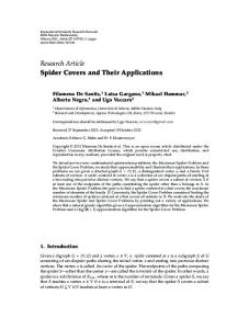
where the Q–dependent part is fully known. The function PQ,Xn ,F can be called the Generalized Power Function. If one minimizes PQ,Xn F (x) for fixed x over all quasi–interpolants Q of the form (6), it turns out that the minimum is attained when the uj are the Lagrange basis of the kernel–based interpolant (4). This yields the standard power function [28] of kernel–based interpolation. We denote it by PXn ,F and use it later. In order to show how the above technique for error bounds works in practice, we add two examples. Example 1. The top left plot of Fig. 1 shows the generalized power function for linear interpolation on the triangle spanned by the three points (0, 0), (1, 0), (0, 1) in R2 . The evaluation is done in the space W22 (R2 ), using the kernel K1 (r)r within the generalized power function, and where Kν is the modified Bessel function of order ν. Note that the kernel–based interpolant using K1 (r)r for interpolation must perform better, but is only slightly superior. The optimal power function is the top right plot, while the difference of the power functions is the lower plot. Example 2. A harder case is given in Fig. 2. In this case, we started from a grid, with spacing h = 0.02, in [−1, 1]2 and we considered only the points falling into the domain of the lower left plot, i.e. 5943 gridded points. Then, the Vandermonde matrix for interpolation by polynomials of degree 6 was formed, and a LU decomposition was calculated which selected 28 points by pivoting [21]. This results in a degree 6 polynomial interpolation method on the circled points of the lower left plot. This polynomial interpolant has an error bound of the above form with the generalized power function for W24 (R) using the kernel K3 (r)r 3 given in the top left plot. The optimal kernel–based interpolation process for the same points in the same function space has the top right power function, while the difference of the power functions is in the lower right plot.

3

Compactly Supported Kernels

First we observe that most of the results in this session are not particularly new. In the univariate case, symmetric even–order B–splines are compactly supported positive definite kernels, because their Fourier transforms are even powers of sinc functions [14]. The multivariate analogues of these would be inverse Fourier transforms of even powers of Bessel functions as arising already in [12], but there are no explicit formulas available. Since 1995, page 5 of 31

R. Schaback, S. De Marchi

November 11, 2009

Figure 1: Error of affine-linear interpolation in W22 however, there are two useful classes of compactly supported kernels due to Z.M. Wu [29] and H. Wendland [27]. The ones by Wendland, having certain advantages, we shall describe below. An addition to the zoo of compactly supported functions was given in 1998 by M.D. Buhmann [1], but we shall focus here on a very recent extension [20] to Wendland’s class of functions. We recall that Wendland’s compactly supported kernels have the form ⌊d/2⌋+k+1

Φd,k (r) = (1 − r)+

· pd,k (r)

(9)

where pd,k is a polynomial of degree ⌊d/2⌋ + 3k + 1 on [0, 1] and such that the kernel K(x, y) = Φd,k (kx − yk2 ) is in C 2k , while pd,k (r) is of minimal degree for smoothness C 2k . Finally, the kernel is reproducing in a Hilbert d/2+k+1/2 space F norm–equivalent to W2 (Rd ). But if the dimension d is even, these functions do not generate integer– order Sobolev spaces. This calls for new compactly supported Wendland– type kernels that work for half–integer k, since it can be expected that d/2+k+1/2 they always generate a space equivalent to W2 (Rd ). In general, the construction of Wendland ’s functions proceeds via φd,k (r) = ψ⌊d/2⌋+k+1,k (r)

(10) page 6 of 31

R. Schaback, S. De Marchi

November 11, 2009

Figure 2: Polynomial interpolation, degree 6. Error in W24 with ψµ,k (r) :=

Z

r

1

t(1 − t)µ

(t2 − r 2 )k−1 dt, 0 ≤ r ≤ 1. Γ(k)2k−1

(11)

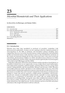
But it turns out that the above formula, used so far only for integers k in order to produce polynomials, can also be used for half–integers k. The R self–explanatory MAPLE code line wend:=int(t*(1-t)^mu*(t*t-r*r)^(k-1)/(GAMMA(k)*2^(k-1)),t=r..1); runs for all reasonable and fixed choices of µ and k where one half–integer is allowed, while it fails if both µ and k are genuine half–integers. A special case is √     p 2 r √ φ2,1/2 (r) = √ 3r 2 log + (2r 2 + 1) 1 − r 2 , 0 ≤ r ≤ 1 3 π 1 + 1 − r2 (12) plotted in Fig. 3 in the one dimensional case. It turns out that it generates a Hilbert space norm–equivalent to W22 (R2 ), as expected. There are a few additional results proven in [20]: page 7 of 31

R. Schaback, S. De Marchi

November 11, 2009

• ψµ,k is positive definite on Rd for µ ≥ ⌊d/2 + k⌋ + 1; • its d–variate Fourier transform for µ = ⌊d/2 + k⌋ + 1 behaves like
O r −(d+2k+1) for r → ∞;

• for d = 2m and k = n + 1/2 the kernel ψ⌊d/2⌋+k+1/2,k generates W2m+n+1 (R2m ); • the new functions have the general form   p r 2 √ ψ2m,n−1/2 (r) = pm−1+n,n (r ) log +qm−1+n,n (r 2 ) 1 − r 2 1 + 1 − r2 (13) with polynomials pm−1+n,n and qm−1+n,n of degree m − 1 + n.

Figure 3: The compactly supported kernel φ2,1/2 (r) Interested readers should work out the case of integer k and half–integer µ, but these functions will not generate new classes of Sobolev spaces. To this end, we suggest to have a look at hypergeometric functions.

4

Expansion Kernels

A kernel K(x, t) =

∞ X

λj ϕj (x)ϕj (t)

(14)

j=0

based on a sequence {ϕj }j≥0 of functions on Ω and a positive sequence {λj }j≥0 of scalars can be called an expansion kernel if the summability page 8 of 31

R. Schaback, S. De Marchi

condition

∞ X j=0

November 11, 2009

λj ϕj (x)2 < ∞ for all x ∈ Ω

(15)

holds. In other contexts, namely in Machine Learning, such kernels are sometimes called Mercer kernels due to their well–known connection to positive integral operators [18] and to the Mercer theorem. But they could also be called Hilbert–Schmidt kernels, because the expansion arises naturally as an eigenfunction expansion of the Hilbert–Schmidt integral operator Z K(x, y)f (y)dy, I(f )(x) := Ω

and Mercer’s theorem just asserts existence of the expansion with positive eigenvalues λj tending to zero for j → ∞, while the eigenfunctions ϕj satisfy I(ϕj ) = λj ϕj , are orthonormal in L2 (Ω) and orthogonal in the native Hilbert space for K. Each continuous positive definite kernel K on a bounded domain Ω has such an expansion, which, however, is hard to calculate and strongly domain–dependent. Thus, Real Analysis allows to rewrite fairly general kernels as expansion kernels, but there also is a synthetic point of view going backwards, namely constructing a kernel from the λj and the ϕj under the summability condition (15). The synthetic approach is the standard one in Machine Learning, and we shall give it a general treatment here, leaving details of kernel construction for Machine Learning to the specialized literature, in particular Part Three of the book [25] by J. Shawe–Taylor and N. Cristianini. In Machine Learning, the domain Ω is a fairly general set of objects about which something is to be learned. The set has no structure at all, since it may consist of texts, images, or graphs, for instance. The functions ϕj associate to each object x ∈ Ω a certain property value, and the full set of the ϕj should map into a weighted ℓ2 sequence space such that the summability condition is satisfied, i.e. into   ∞   X λj |cj |2 < ∞ ℓ2,Λ := {cj }j≥0 :   j=0

with the inner product

({aj }j≥0 , {bj }j≥0 )ℓ2 ,Λ :=

∞ X

λj aj bj .

j=0

page 9 of 31

R. Schaback, S. De Marchi

November 11, 2009

The map x 7→ {ϕj (x)}j≥0 ∈ ℓ2,Λ is called the feature map. In specific applications, there will only be finitely many functions comprising the feature map, but we focus here on the infinite case. To proceed towards a Hilbert space of functions for which K is reproducing, one should look at the sequence ΛΦ(x) := {λj ϕj (x)}j≥0 of coefficients of the function K(x, ·) for fixed x ∈ Ω. This sequence lies in the space ℓ2,Λ−1 with an inner product defined as above but using λ−1 instead of λj . Thus we should look at expansions j into the ϕj such that the coefficient sequences lie in ℓ2,Λ−1 . If the feature functions ϕj are linearly dependent, there are problems with non-unique coefficients for expansions into the ϕj . To handle this in general, we refer the reader to the use of frames, as done in R. Opfer’s dissertation [15]. Instead, we now assume linear independence of the ϕj over Ω and define a space of functions     X c2j (f ) X 0, N ⊆ N (j!)2

(27)

with the summability condition (15) taking the form X

j∈N

λj

x2j < ∞ for all x ∈ Ω (j!)2 page 16 of 31

R. Schaback, S. De Marchi

November 11, 2009

will be admissible here, and we allow the set N ∈ N≥0 to be infinite but otherwise arbitrary. Depending on the weights λj , the domain Ω can be all R or just an interval. The connection to expansion kernels is via ϕj (x) = xj /j!, and Section §4 teaches us that the native space F consists of all functions f of the form f (x) =

X

j∈N

cj

X c2j xj with < ∞. j! λj j∈N

Then cj = f (j)(0) leads to the space ) ( X (f (j) (0))2 X xj (j) for all x ∈ Ω, 0 such that for any discrete set X ⊂ I = [−a, a] with fill distance h ≤ h0 and any function f ∈ FR , the error between f and its rational interpolant of the form X 1 (30) sf,X (t) := αj 1 − t xj xj ∈X

on the set X, is bounded by kf − sf,X kL∞ [−a,a] ≤ e−c1 /h kf kFR .

7

(31)

Periodic Kernels

For spaces of 2π–periodic functions, there are some nice and useful kernels. We list now some interesting examples.

page 18 of 31

R. Schaback, S. De Marchi

November 11, 2009

Example 8. Consider ∞ X 1 cos(n(x − y)) = n2

n=1

1 1 1 (x − y)2 − π(x − y) + π 2 4 2 6

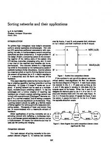
for x − y ∈ [0, 2π] with periodic extension. Notice that the above series is a polynomial of degree 2 in x − y. An example is provided in the top left plot of Fig. 7. Example 9. In more generality, the functions ∞ X 1 cos(n t) n2k

(32)

n=1

represent polynomials of degree 2k on [0, 2π]. To see this, consider Hurwitz-Fourier expansions Bm (x) = −

m! (2πi)m

+∞ X

n−m e2πinx

n=−∞, n6=0

of the Bernoulli polynomials Bm of degree m on [0, 1] (for details see, e.g. http://mathworld.wolfram.com/BernoulliPolynomial.html). If we set t = 2πx and m = 2k, we get t ) B2k ( 2π

(2k)! (2π)2k

+∞ X

n−2k (cos(nt) + i sin(nt))

=

(−1)k+1

=

n=−∞, n6=0 +∞ (2k)! X −2k 2(−1)k+1 n cos(nt) (2π)2k n=1

that proves our claim. Example 10. But there are still some other nice cases due to A. Meyenburg [9], namely ∞ X 1 cos(n(x − y)) = cos(sin(x − y)) · exp(cos(x − y)) n! n=0 ∞ X 1 − 21 cos(x − y) 1 cos(n(x − y)) = 2n 1 − cos(x − y) + 14 n=0

(33)

page 19 of 31

R. Schaback, S. De Marchi

November 11, 2009

2

3

1.5

2.5

1

2

0.5

1.5

0

1

−0.5

0.5

−1

−5

0

0

5

7

0

5

−5

0

5

4.5

6

4

5

3.5

4

3

3

2.5

2

2

1

1.5

0

−5

−5

0

1

5

Figure 7: Periodic kernels depicted in Fig. 7 on the top right and bottom left, and ∞

4 X 1 − (−1)n e−2π exp(−2|x|) = cos(nx), π 4 + n2  n=0 4−x 0≤ x  K(x) := 8 − 2π 2π − 4 < x  4 − 2π + x 4≤ x ∞ 2 X 4 sin (2n) 16 + cos(nx). = π πn2

x ∈ [−π, π], ≤ 2π − 4