Word-Sequence Kernels - CiteSeerX

Journal of Machine Learning Research 3 (2003) 1059-1082

Submitted 4/02; Published 2/03

Word-Sequence Kernels Nicola Cancedda Eric Gaussier Cyril Goutte Jean-Michel Renders

N ICOLA .C ANCEDDA @ XRCE . XEROX . COM E RIC .G AUSSIER @ XRCE . XEROX . COM C YRIL .G OUTTE @ XRCE . XEROX . COM J EAN -M ICHEL .R ENDERS @ XRCE . XEROX . COM

Xerox Research Centre Europe 6, chemin de Maupertuis 38240 Meylan, France

Editors: Jaz Kandola, Thomas Hofmann, Tomaso Poggio and John Shawe-Taylor

Abstract We address the problem of categorising documents using kernel-based methods such as Support Vector Machines. Since the work of Joachims (1998), there is ample experimental evidence that SVM using the standard word frequencies as features yield state-of-the-art performance on a number of benchmark problems. Recently, Lodhi et al. (2002) proposed the use of string kernels, a novel way of computing document similarity based of matching non-consecutive subsequences of characters. In this article, we propose the use of this technique with sequences of words rather than characters. This approach has several advantages, in particular it is more efficient computationally and it ties in closely with standard linguistic pre-processing techniques. We present some extensions to sequence kernels dealing with symbol-dependent and match-dependent decay factors, and present empirical evaluations of these extensions on the Reuters-21578 datasets. Keywords: Kernel machines, text categorisation, linguistic processing, string kernels, sequence kernels

1. Introduction The application of machine learning techniques to classification of documents is a rich and challenging research area with many related tasks, such as routing, filtering or cross-lingual information retrieval. Since Joachims (1998) and other researchers like Yang and Liu (1999) have shown that Support Vector Machines (SVM) perform favourably compared to competing techniques for document categorisation, kernel machines have been a popular choice for document processing. In most reported works, however, documents were represented using the standard vector space, aka bag-of-word model (Salton and McGill, 1983)—that is, more or less, word frequencies with various added normalisations—in conjunction with general purpose kernels (linear, polynomial, RBF, etc.). Recently, Watkins (1999) and Lodhi et al. (2001, 2002) proposed the use of string kernels, one of the first significant departures from the vector space model. In string kernels, the features are not word frequencies or an implicit expansion thereof, but the extent to which all possible ordered subsequences of characters are represented in the document. In addition, Lodhi et al. (2001) proposed a recursive dynamic programming formulation allowing the practical computation of the similarity between two sequences of arbitrary symbols as the dot-product in the implicit feature space of all ordered, non-consecutive subsequences of symbols. Although it allows to perform the kernel calculation without performing an explicit feature space expansion, this formulation is extremely computationally demanding and is not applicable (with current processing power) to large document collections without approximation (Lodhi et al., 2002). In this document, we propose to extend the idea of sequence kernels to process documents as sequences of words. This greatly expands the number of symbols to consider, as symbols are words rather than characters, but it reduces the average number of symbols per document. As the dynamic programming formulation used for computing sequence matching depends only on sequence length, this yields a significant improvement in computing efficiency. Training a SVM on a dataset of around 10000 documents like the Reuters-21578

c 2003 Nicola Cancedda, Eric Gaussier, Cyril Goutte and Jean-Michel Renders.

C ANCEDDA , G AUSSIER , G OUTTE AND R ENDERS

corpus becomes feasible without approximation. In addition, matching sequences of words allows to work with symbols that are expected to be more linguistically meaningful. This leads to extensions of the word sequence kernels that implement a kind of inverse document frequency (IDF) weighting by allowing symbolvarying decay factors. Words may also be equivalent in some context, and we show how to implement soft word matching in conjunction with the word-sequence kernel. This allows the use of this kernel in a multilingual context, an application that was not possible with the string kernel formulation. In Section 2 we offer a brief self-contained introduction to kernel methods, after which we will proceed with the presentation of sequence kernels (Section 2.2). Section 3 formulates and verifies a hypothesis that helps explain why string kernels perform well, even though they are based on processing entities (characters) which are essentially meaningless from a linguistic point of view. Section 4 presents our extension of sequence kernels to word-sequences, which we test empirically in Section 4.2. Finally, we present in Section 5 some extensions of word-sequence kernels to soft-matching and cross-lingual document similarity.

2. Kernel Methods Kernel methods are a research field in rapid expansion. Based on theoretical work on statistical learning theory (Vapnik, 1995) and reproducing kernel Hilbert spaces (Wahba, 1990), kernel machines were first popular as SVM (Boser et al., 1992, Cortes and Vapnik, 1995). In this section we will briefly introduce kernel-based classifiers and sequence kernels. For additional information, the reader may refer to general introductions such as Cristianini and Shawe-Taylor (2000), Sch¨olkopf and Smola (2002) or Herbrich (2002). 2.1 Kernel Classifiers A binary classifier is a function from some input space X into the set of binary labels {−1, +1}. A supervised learning algorithm is a function that assigns, to each labeled training set S ∈ (X × {−1, +1}) l , a binary classifier h : X → {−1, +1}. For computational reasons and in order to limit overfitting, learning algorithms typically consider only a subset of all classifiers, H ⊂ {h | h : X → {−1, +1}}, the hypothesis space. In the common case in which X is a vector space, one of the simplest binary classifiers is given by the linear discriminant: h(x) = sign(w, x + b) where ·, · denotes the standard dot-product. Learning the linear classifier amounts to finding values of w and b which maximise some measure of performance. Learning algorithms for linear classifiers include e.g. Fisher’s linear discriminant, the Perceptron and SVM. All linear classifiers will naturally fail when the boundary between the two classes is not linear. However, it is possible to leverage their conceptual simplicity by projecting the data from X into a different feature space F in which we hope to achieve linear separation between the two classes. Denoting the projection into feature space by φ : X → F , the generalised linear classifier becomes: h(x) = sign (w, φ(x) + b) (1) The separating hyperplane defined by w and b is now in the feature space F , and the corresponding classifier in the input space X will generally be non-linear. Note also that in this setting, X need not even be a vector space as long as F is. This is a crucial observation for the rest of this article, as we will be dealing with the case in which X is the associative monoid of the sequences over a fixed alphabet, which is not a vector space. can be expressed as a linear combination of the data: In the case of SVM, the optimal weights w l

= ∑ yi αi φ(xi ) w

(2)

i=1

where αi ∈ R is the weight of the i-th training example with input x i ∈ X and label yi ∈ {−1, +1}. Accordingly, by combining (1) and (2), the SVM classifier can be written in its dual form: h(x) = sign

l

∑ yi αi φ(x), φ(xi ) + b

i=1

1060

(3)

W ORD -S EQUENCE K ERNELS

Notice that the projection φ only appears in the context of a dot product in (3). In addition, the optimal weights (αi ) are the solution of a high dimensional quadratic programming problem which can be expressed in terms of dot products between projected training data φ(x i ), φ(x j ). Rather than use the explicit mapping φ, we can thus use a kernel function K : X × X → R such that K(x, y) = φ(x), φ(y). As long as K(x, y) can be calculated efficiently, there is actually no need to explicitly map the data into feature space using φ —this is the kernel trick. It is especially useful when the computational cost of calculating φ(x) is overwhelming (e.g., when F is high dimensional) while there is a simple expression for K(x, y). In fact, Mercer’s theorem (see, e.g. Cristianini and Shawe-Taylor, 2000, Section 3.3.1) states that any positive semi-definite symmetric function of two arguments corresponds to some mapping φ in some space F and is thus a valid kernel. This means that in principle a kernel can be used even if the nature of the corresponding mapping φ is not known. This article addresses the application of kernel methods to the well known problem of document categorisation. So far, most of the kernel-based work in this area used a standard bag-of-words representation, with word frequencies as features, ie X = R n . Although these vector representations have proved largely successful, we will here investigate the use of representations which are intuitively closer to the intrinsic nature of documents, namely sequences of symbols. This representation does not form a vector space, but the use of appropriate kernels will allow us to leverage the discriminative power of kernel-based algorithms. As we will see, the kernels we are going to consider will also allow us to test basic factors (e.g., order or locality of multi-word terms) in the context of document categorisation. 2.2 Sequence Kernels The assumption behind the popular bag-of-words representation is that the relative position of tokens has little importance in most Information Retrieval (IR) tasks. Documents are just represented by word frequencies (and possibly additional weighting and normalisation), and the loss of the information regarding the word positions is more than compensated for by the use of powerful algorithms working in vector space. Although some methods inject positional information using phrases or multi-word units (Perez-Carballo and Strzalkowski, 2000) or local co-occurrence statistics (Wong et al., 1985), the underlying techniques are based on a vector space representation. String kernels (or sequence kernels) are one of the first significant departures from the vector-space representation in this domain. String kernels (Haussler, 1999, Watkins, 1999, Lodhi et al., 2001, 2002) are similarity measures between documents seen as sequences of symbols (e.g., possible characters) over an alphabet. In general, similarity is assessed by the number of (possibly non-contiguous) matching subsequences shared by two sequences. Non contiguous occurrences are penalized according to the number of gaps they contain. Formaly, let Σ be a finite alphabet, and s = s 1 s2 . . . s|s| a sequence over Σ (i.e. s i ∈ Σ, 1 ≤ i ≤ |s|). Let i = [i1 , i2 , . . . , in ], with 1 ≤ i1 < i2 < . . . < in ≤ |s|, be a subset of the indices in s: we will indicate as s[i] ∈ Σ n the subsequence s i1 si2 . . . sin . Note that s[i] does not necessarily form a contiguous subsequence of s. For example, if s is the sequence CART and i = [2, 4], then s[i] is AT . Let us write l(i) the length spanned by s[i] in s, that is: l(i) = in − i1 + 1. The sequence kernel of two strings s and t over Σ is defined as: Kn (s,t) =

∑n ∑ ∑

λl(i)+l(j)

(4)

u∈Σ i:s[i]=u j:t[j]=u

where λ ∈]0; 1] is a decay factor used to penalise non-contiguous subsequences and the first sum refers to all possible subsequences of length n. Equation 4 defines a valid kernel as it amounts to performing an inner product in a feature space with one feature per ordered subsequence u ∈ Σ n with value: φu (s) =

∑

λl(i)

(5)

i:s[i]=u

Intuitively, this means that we match all possible subsequences of n symbols, even when these subsequences are not consecutive, and with each occurrence “discounted” according to its overall length.

1061


A direct computation of all the terms under the nested sum in (4) becomes impractical even for small values of n. In addition, in the spirit of the kernel trick discussed in Section 2, we wish to calculate K n (s,t) directly rather than perform an explicit expansion in feature space. This can be done using a recursive formulation proposed by Lodhi et al. (2001), which leads to a more efficient dynamic-programming-based implementation. The derivation of this efficient recursive formulation is given in appendix A, together with an illustrative example. It results in the following equations: K0 (s,t) Ki (s,t) Ki (s,t) Ki (sx,ty) Ki (sx,tx) Ki (sx,t) Kn (s,t) Kn (sx,t)

= 1, for all s,t, for all i = 1, . . . , n − 1: = 0, if min(|s|, |t|) < i

(6)

= 0, if min(|s|, |t|) < i = λKi (sx,t) iff y = x

(7) (8)

= λKi (sx,t) + λ2Ki−1 (s,t) = λKi (s,t) + Ki (sx,t)

otherwise

and finally: = 0, if min(|s|, |t|) < n = Kn (s,t) +

∑

j:t j =x

λ

2

Kn−1 (s,t[1

(9) (10) (11)

: j − 1])

(12)

The time required to compute the kernel according to this formulation is O(n|s||t|). In some situations, it may be convenient to perform a linear combination of sequence kernels with different values of n. Using the recursive formulation, it turns out that computing all kernel values for subsequences of lengths up to n is not significantly more costly than computing the kernel for n only. In order to keep the kernel values comparable for different values of n and to be independent from the length of the strings , it may be advisable to consider the normalised version: K(s,t) ˆ K(s,t) = (13) K(s, s)K(t,t) This is a generalisation of the “cosine normalisation” which is widespread in IR and corresponds to the ˆ = φ(s) (where . 2 is the 2-norm). mapping φ(s)

φ(s)

2

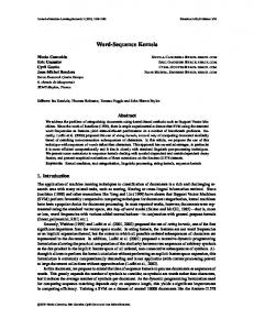
3. The Noisy-Stemming Hypothesis Text categorisation using string kernels operating at the character level has been shown to yield performance comparable to kernels based on the traditional bag-of-words representation (Lodhi et al., 2001, 2002). This result is somewhat surprising, considering string kernels use only low-level information. A possible explanation of the effectiveness of the string kernel, supported by the observation that performance improves with n, is that subsequences most relevant to the categorisation may correspond to noisy versions of word stems, thus implicitly implementing some form of morphological normalisation. Furthermore, as gaps within the sequence are allowed —although penalized— string kernels could also pick up stems of consecutive words, as illustrated in Figure 1. This is known to help in IR applications (Salton and McGill, 1983). In order to test this noisy stemming hypothesis, the following experiment was conducted. An SVM using a string kernel was trained on a small subset of the Reuters-21578 corpus, 1 using the labels for the acq topic. A sample of features—subsequences of a fixed length n—was randomly chosen. In order to avoid a vast majority of irrelevant low-weight features, we restricted ourselves to possibly non-contiguous subsequences appearing in the Support Vectors. For each sampled feature u, its impact on the categorisation decision was compared to a measure of stemness σ u . The impact on the categorisation decision is measured by the absolute 1. Available at http://www.daviddlewis.com/resources/testcollections/reuters21578/. The subset is built from the first 114 documents with the acq label and the first 266 documents not in acq.

1062


4−GRAMS P RI CE

OF

CORN

E X P ORT A

5−GRAMS I S H

A

J OI NT

V E NT URE

W

Figure 1: The noisy-stemming hypothesis. N-grams may be able to pick parts of words/stems (top, with n = 4) or even pick parts of stems of consecutive words (bottom, n = 5).

weight wu in the linear decision:

wu = ∑ α j y j φu (x j ) j

In order to assess the stemness of a feature, ie the extent to which a feature approximates a word stem, a simplifying assumption was made by considering that stems are the initial characters in a word. Moreover, in order to verify that a feature may span two consecutive stems, a measure of stemness was devised so as to consider pairs of consecutive tokens. Let t = {t 1 , ...,tm }, with 1 = t1 < t2 < ... < tm < tm+1 = |s| + 1, be a tokenisation of the string s (the tokenisation is the segmentation process that provides the indices of the first symbol of each token). Let m(k, u) be the set of all matches for the subsequence u in the pair of consecutive tokens starting in t k−1 and tk respectively, with 2 ≤ k ≤ m: m(k, u) = i , i |u = s[i ]s[i ],tk−1 ≤ i 1 ≤ i |i | < tk ≤ i 1 ≤ i |i | < tk+1 / the constraint tk−1 ≤ i |i | < tk is considered automatically satisfied. In In a matching pair where i = 0, / in order to avoid double counting of single word matches, and addition, i is forced to be different from 0, an empty symbol is added at the beginning of the string to allow one-word matching on the first token. The stemness of a subsequence u with respect to s is then defined as:

minm(k,u) i |i | −tk−1 −|i |+i |i | −tk −|i | σu (s) = avgk:m(k,u) =0/ λ In other words, for each pair of consecutive tokens containing a match for u, a pair of indices (i , i ) is selected such that s[i ] matches into the first token, s[i ] matches in the second and each component is found as compact and close to the start of the corresponding token as possible. The stemness of u with respect to the whole training corpus is then defined as the (micro-)average of the stemness in all documents in the corpus. This experiment was performed with a sample of 15000 features of length n = 3, and a sample of 9000 features of n = 5, with λ = 0.5 in both cases. Under the noisy-stemming hypothesis, we expect relatively few features with high weight and low stemness. The outcome of our experiment, presented in Table 1, seems to confirm this. For n=3, among features with high weight (> 0.15) about 92% have high stemness, whereas among features with low weight the fraction of features with high stemness is of 73%. Similar results were found for n = 5 (90% and 46% respectively). / stemness is calculated For each non-empty set of matches by first finding the most compact m(k, u) = 0, match (ic , ic ) = argmin(i ,i )∈m(k,u) i |i | − tk−1 − |i | + i |i | − tk − |i | . It is interesting to check how often this “minimal” subsequence matches on two tokens, as opposed to single-token match. For that purpose, we / and g(k, u) = 2 otherwise. The define g(k, u) = 1 if the most compact match is on one token (i.e. i c = 0) multigramness of a subsequence u on sequence s is then: γu (s) = avgk:m(k,u) =0/ (g(k, u)) 1063


n=3 σu low high

n=5 σu low high

wu low 3622 9877

high 125 1376

wu low high 4413 86 3686 815

Table 1: Contingency tables for weight against stemness. Left (n = 3, ie trigrams): Weights are split at 0.15 to separate the lowest 90% and highest 10% values, whereas stemness is split at 0.064 to separate the 25% lowest and 75% highest values. Right (n = 5): Weights are split at 0.0066 to separate the lowest 90% and highest 10% values, whereas stemness is split at 0.029 to separate the 50% lowest and 50% highest values. The χ 2 values for the tables are 247 (left) and 655 (right), which suggests a highly significant departure from independence in both cases (1 d.o.f.).

8 6 2 0 1.0

1.2

1.4

1.6

1.8

2.0

1.0

1.2

1.4

1.6

1.8

2.0

High Weight & High Stem (n=5)

High Weight & Low Stem (n=5)

30 20 0

0

10

20

Density

30

40

Multigramness

40

Multigramness

10

Density

4

Density

6 4 0

2

Density

8

10

High Weight & Low Stem (n=3)

10

High Weight & High Stem (n=3)

1.0

1.2

1.4

1.6

1.8

2.0

Multigramness

1.0

1.2

1.4

1.6

1.8

2.0

Multigramness

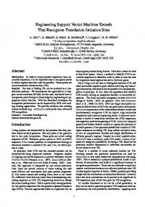
Figure 2: Density of “Multigramness” for high weight features, n = 3 and n = 5. Using the same feature samples as above, we estimate the distribution of γ u (s) for features with high weights (the most interesting features). Figure 2 shows that the mass of each distribution is close to 2, indicating that matching occurs more often on more than one word. This effect is even clearer for larger n: high weight features of length n = 5 are concentrated near γ u = 2. This is reasonable considering longer subsequences are harder to match on a single word. On the other hand, a significant amount of high weight, high stemness features of length n = 3 are clearly single stem features. In addition, features with high weight but low stemness have a tendency to spread on two stems (right column vs. left column in Figure 2). This suggests that multiple word matching really does occur and is beneficial in forming discriminant, high weight features. This is also in agreement with results on SVM using traditional kernels (Joachims, 1998) showing that polynomial kernels consistently outperform the linear kernel.

1064


4. Word-Sequence Kernels The seeming validity of the noisy-stemming hypothesis suggests that sequence kernels operating at the word (possibly word-stem) level might prove more effective than those operating at the character level. In this section, we describe the impact of applying sequence kernels at the word level, and extend the original kernel formulation so as to take into account additional information. 4.1 Theory The direct application of the sequence kernel defined above on an alphabet of individual words raises some significant issues. First, the feature space on which documents are implicitly mapped has one dimension for each of the |Σ|n ordered n-tuples of symbols in the alphabet: going from characters to words, the order of magnitude of |Σ| increases from the hundreds to the tens of thousands, and the number of dimensions of the feature space increases accordingly. However, the average length in symbols of documents decreases by an order of magnitude. As the algorithm used for computing sequence kernels depends on sequence length and not on alphabet size, this yields a significant improvement in computing efficiency: word-sequence kernels can be computed on datasets for which string kernels have to be approximated. Nevertheless, the combination of the two effects (increase in alphabet size, decrease in document average length) causes documents to have extremely sparse implicit representations in the feature space. This in turn means that the kernel-based similarity between any pair of distinct documents will tend to be small with respect to the “self-similarity” of documents, especially for larger values of n. In other words, the Gram matrix tends to be nearly diagonal, meaning that all examples are nearly orthogonal. In order to overcome this problem, it is convenient to replace the fixed-length sequence kernel with a combination of sequence kernels with subsequence lengths up to a fixed n. A straightforward formulation is the following 1-parameter linear combination: n (14) K¯n (x, y) = ∑ µ1−i Kˆi (x, y) i=1

Considering the dynamic programming technique used for the implementation, computing the sequence kernel for subsequences of length up to n requires only a marginal increase in time compared to the computation for subsequences of length n only. Notice that kernel values for different subsequence lengths are normalised independently before being combined. In this way it is possible to control the relative weight given to different subsequence lengths directly by means of the parameter µ. The µ parameter, or possibly the parameters of a general linear combination of sequence kernels of different orders, can be optimized by cross-validation, or alternatively by kernel alignment (Cristianini et al., 2001). In its original form, the sequence kernel relies on mere occurrence counts, or term frequencies, and lacks feature weighting schemes which have been deemed important by the IR community. We want to present now two extensions to the standard sequence kernel. The first uses different values of λ to assign different weights to gaps, and allows the use of well-established weighting schemes, such as the inverse document frequency (IDF). It can also be used to discriminate symbols according to, say, their part-of-speech. The second extension consists in adopting different decay factors for gaps and for symbol matches, and generalises over the previous extension in the sense that informative symbols are treated differently depending on whether they are used in matches or gaps. 4.1.1 S YMBOL -D EPENDENT D ECAY FACTORS The original formulation of the sequence kernel uses a unique decay factor λ for all symbols. It can well be the case, however, that sequences containing some symbols have a significantly better discriminating power than sequences containing other symbols. For example, a sequence made of three nouns is more likely to be more informative than a sequence made of a preposition, a determiner and a noun. A way to leverage on this non-uniform discriminative power consists in assigning different decay factors to distinct symbols. We thus

1065


introduce a distinct λ x for each x ∈ Σ. This induces the following new embedding: φu (s) =

∑

∏

i:s[i]=u i1 < j