develop a normal bisimulation that characterizes barbed congruence, in the strong and weak cases, ...... for higher order processes. Acta Informatica, 30(1), 1993.
Normal Bisimulations in Calculi with Passivation Sergue¨ı Lenglet1 , Alan Schmitt2 , and Jean-Bernard Stefani2 1
Universit´e Joseph Fourier, Grenoble, France 2 INRIA Grenoble-Rhˆ one-Alpes, France
Abstract. Behavioral theory for higher-order process calculi is less well developed than for first-order ones such as the π-calculus. In particular, effective coinductive characterizations of barbed congruence, such as the notion of normal bisimulation developed by Sangiorgi for the higherorder π-calculus, are difficult to obtain. In this paper, we study bisimulations in two simple higher-order calculi with a passivation operator, that allows the interruption and thunkification of a running process. We develop a normal bisimulation that characterizes barbed congruence, in the strong and weak cases, for the first calculus which has no name restriction operator. We then show that this result does not hold in the calculus extended with name restriction.
1
Introduction
Motivation A natural notion of behavioral equivalence for process calculi is barbed congruence. Informally, two processes are barbed-congruent if they behave in the same way (i.e., have the same reductions and the same observables) when placed in similar, but arbitrary, contexts. Due to this quantification on contexts, barbed congruence is unwieldy to use in proofs of equivalence, or to serve as a basis for automated verification tools. One is thus lead to study coinductive characterizations of barbed congruence, typically in the form of bisimilarity relations. For first-order process calculi, such as the π-calculus and its variants, the resulting behavioral theory is well developed, and one can in general readily define bisimilarity relations that characterize barbed congruence. For higher-order process calculi, the situation is less satisfactory. Simple higher-order calculi, such as HOπ [10, 11], have a well-studied behavioral theory. For HOπ, Sangiorgi has defined context and normal bisimilarity relations, which both are sound with respect to barbed congruence (i.e. are included in barbed congruence) and sometimes complete (i.e. they contain barbed congruence), leading to a full characterization. However, context bisimilarity still involves some quantification over test contexts. For instance, when assessing the equivalence of two processes which consist only of the output of a message on a communication channel a, context bisimilarity needs to consider every interacting system that is capable of doing an input on channel a. Normal bisimilarity improves context bisimilarity by requiring only a single test context. E.g., in the case of two emitting processes, as above, normal bisimilarity only requires to compare the behavior of the two processes when placed in parallel with a single particular
receiving process. Furthermore, context and normal bisimilarities characterize barbed congruence both in the strong case (where internal steps are observable), and in the weak case (where internal steps are not observable). Unfortunately, HOπ is not expressive enough to faithfully model concurrent systems with dynamic reconfiguration or strong mobility capabilities. For instance, a running HOπ process cannot be stopped, which prevents the faithful modeling of process failures, of online process replacement, or of strong process mobility. It is for this reason that we have seen the emergence of process calculi with (forms of) process passivation. Process passivation allows a named process to be stopped and its state captured at any time during its execution. The Kell calculus [13] and Homer [5] are examples of higher-order process calculi with passivation. The behavioral theory of these calculi is less understood than the one for HOπ, whose proof techniques and relations do not carry over. No sound and complete characterization of barbed congruence has been found in the weak case for these calculi. Importantly, no relation akin to normal bisimilarity has been developed. Contributions To pinpoint issues that arise in the development of a behavioral theory for higher-order calculi with passivation, and to show that they arise from the interplay between passivation and restriction, we consider in this paper two calculi with passivation, which are simpler than both Homer and the Kell calculus, and which differ merely in the presence of restriction. The first one, called HOP, extends HOcore with passivation and sum. HOcore is a minimal higher-order concurrent calculus without restriction that has recently been studied in [7]. As a first contribution, we show that HOP admits a sound and complete form of normal bisimulation, in both the strong and weak cases. The second calculus, called HOπP, extends HOπ with passivation. As a second contribution, we show that with HOπP a large class of tests does not suffice to build a sound normal bisimulation. This casts some doubt as to whether a suitable notion of normal bisimilarity, that is with finite testing, can be found for HOπP, and therefore for Homer and the Kell calculus. Summary In Section 2, we define HOπP and recall the previous works on behavioral equivalences in the Kell calculus and Homer. We define in Section 3 a sound and complete normal bisimilarity for HOP. We show in Section 4 that this relation is not suitable for HOπP. We discuss related work in Section 5, and Section 6 concludes the paper. The paper only contains proof sketches for some results. Complete proofs can be found in [8].
2
Bisimulations in HOπP
Studying proof techniques for establishing contextual equivalence in calculi such as Homer and the Kell calculus has been the main motivation for this work. Instead of working directly in one of these calculi, we consider a simpler calculus, HOπP (for Higher-Order π with Passivation), which extends the HOπ calculus
Agents: Variables, names: P, Q, R, S: Processes m, n, m, n, . . .: first-order names and co-names F, G: Abstractions a, b, a, b, . . .: higher-order names and co-names C, D: Concretions x, y: first or higher-order names A, B: Agents X, Y : process variables Actions: τ : Internal action l ∈ {m, m, . . .} ∪ τ : first-order actions α ∈ {m, m, . . .} ∪ τ ∪ {a, a, . . .}: first or higher-order actions Syntax: P ::= 0 | X | P | P | l.P | a(X)P | ahP iP | νx.P | !P | a[P ] Fig. 1. Meta-Variables and Syntax of HOπP
studied in [11] with a passivation operator, and which exhibits the same technical difficulties encountered in Homer and Kell. 2.1
Syntax and Transition Semantics
Meta-variables and syntax of HOπP are given Figure 1. We add localities a[P ] to the HOπ constructs. These are passivation units. As long as no passivation occurs, a locality a[P ] is a transparent evaluation context: the process P may evolve and communicate freely with processes outside of a, independently of their position in the locality tree. At any time, passivation may be triggered and the process a[P ] becomes a concretion hP i0. Passivation may thus occur as an internal τ step only if there is a receiver on a ready to receive the contents of the locality. The receiver may then choose to spawn, forward, or discard the process. Name restriction νx.P makes the name x private to process P . We write bn(P ) (resp. fn(P )) for the bound names (resp. free names) of P . Message input a(X)P binds the variable X in P . We write fv(P ) for the free process variables of a process P . A process P is said to be closed if fv(P ) = ∅. We identify processes up to α-conversion of names and variables. Structural congruence ≡ is the smallest congruence verifying the following laws. P | (Q | R) ≡ (P | Q) | R νx.0 ≡ 0
P |Q≡Q|P
!P ≡ P |!P
P |0≡P
νx.νy.P ≡ νy.νx.P
νx.(P | Q) ≡ P | νx.Q (x ∈ / fn(P ))
We now give an informal account of the labeled transition semantics (LTS) α − → of the calculus. There are three kinds of transitions: first-order transition, l higher-order input, and higher-order output. In a first-order transition P → − Q, processes may evolve towards processes by an internal action τ , or by a firstorder input or output (labeled by the corresponding name or co-name). In the a higher-order input P − → F = (X)Q, P evolves towards an abstraction F , which states that it may receive a process R on name a to continue as Q{R/X}. In
a
the higher-order output P − → C = νe x.hRiS, P evolves towards a concretion C, which states that it may send process R on name a and continue as S, and the scope of names x e (such that x e ⊆ fn(R)) has to be expanded to encompass the recipient of R. We call the set x e the bound names of C, written bn(C). A higher-order communication takes place when a concretion interacts with an abstraction. We define a pseudo-application operator • between F and C above ∆ by F • C = νe x.(Q{R/X} | S) (with fn(Q) ∩ x e = ∅). Let the set of agents, written A, be the set of all processes, abstractions, and concretions. We extend restriction, parallel composition, and locality to all agents. Let F = (X)P be an abstraction, we then have νx.F = (X)νx.P and a[F ] = (X)a[P ]. If X ∈ / fv(Q), then F | Q = (X)(P | Q) and Q | F = (X)(Q | P ). Let C = ν ye.hQiR be a concretion and x ∈ / ye. If x ∈ fn(Q), then νx.C = νx, ye.hQiR, otherwise νx.C = ν ye.hQiνx.R. If ye ∩ fn(P ) = ∅, then C | P = ν ye.hQi(R | P ) and P | C = ν ye.hQi(P | R). If a 6∈ ye, then a[C] = ν ye.hQia[R]. The LTS rules are given in Figure 2, with the exception of the symmetric rules for LTS-Par, LTS-FO, and LTS-HO. According to rule LTS-Loc, a locality a[P ] becomes a concretion when P outputs a message and becomes a concretion. Since the bound names of a concretion are extruded “by need” to encompass the receiving process, their scope may thus cross locality boundaries. Remark 1. Passivation in HOπP can be seen as objective, as it requires a receiver on the locality’s name to result in a silent τ step.
l l.P − → P LTS-Prefix
a
a(X)P − → (X)P LTS-Abstr α
P − →A
a
ahQiP − → hQiP LTS-Concr α
P − →A
α
α∈ / {x, x}
νx.P − → νx.A m
P |!P − →A LTS-Restr
α
m
P −→ P 0
0
0
P |Q− →P |Q
!P − →A a
P − →F LTS-FO
LTS-Replic
α
a
Q −→ Q0 τ
LTS-Par
α
→A|Q P |Q−
Q− →C τ
P |Q− →F •C
LTS-HO
α
P − →A α
a[P ] − → a[A]
LTS-Loc
a a[P ] − → hP i0 LTS-Passiv
Fig. 2. Labeled Transition System for HOπP
2.2
Strong Behavioral Equivalences
Barbed congruence is a uniform definition of process equivalence among process ∆ τ calculi based on the reduction relation −→ (defined as −→ = ≡− →≡), the observable actions of a process, called barbs, and contexts. In HOπP, a process P has µ a barb µ = x | x, written P ↓µ , iff we have P − →. Contexts are processes with a hole 2; filling a context C with a process P gives a process written C{P }. Definition 1. A relation R on closed processes is a strong barbed bisimulation iff R is symmetric, and P R Q implies: – If P ↓µ then Q ↓µ – If P −→ P 0 , then there exists Q0 such that Q −→ Q0 and P 0 R Q0 . Processes P and Q are strongly barbed congruent, written P ∼b Q, iff for all contexts C, there exists a strong barbed bisimulation R such that C{P } R C{Q}. The universal quantification over contexts makes barbed congruence difficult to use in practice. Sangiorgi introduced context bisimilarity for HOπ [11] as an LTS-based alternative to barbed congruence. Context bisimilarity is sound, i.e. is included in barbed congruence. In the weak case, there exists a version (”early non delay”) of the bisimilarity which is also complete, i.e. contains barbed congruence, and therefore is a characterization of weak barbed congruence (see [10] for further details). We write B for the strong context bisimilarity of HOπ (see [11] for the definition). Using this bisimilarity with HOπP leads to a relation which is not sound: there exist HOπP processes related by B which are not strong barbed congruent. Consider the following processes: P0 = ah0i!m.0
Q0 = ahm.0i!m.0
Processes P0 and Q0 are related by B: the difference between the emitted messages is shadowed by the continuation !m.0. They cannot be distinguished by a HOπ context, but are distinguished by an HOπP context which may discard the message continuations: C = b[2] | a(X)X | b(X)0. With a communication on a followed by passivation/communication on b, we have C{P0 } −→ b[!m.0] | 0 | b(X)0 −→ 0. It can only be matched by C{Q0 } −→ b[!m.0] | m.0 | b(X)0 −→ m.0. The two resulting processes have different barbs, therefore P0 and Q0 are not barbed congruent. Hence relation B is not sound with HOπP. In a concretion νe x.hRiS, the emitted process R may be sent outside a locality b while the continuation S stays in b. If the passivation on b is triggered, S may be destroyed (as with P0 and Q0 ) or put in a different context. Hence the passivation may separate the processes R and S and put them in totally different contexts, which is not possible in a calculus without passivation. As in the Kell calculus and Homer, we address this issue by testing messages and continuations in different evaluation contexts E. These contexts, when applied to concretions, take into account the fact that a message and its continuation are separated: in the definition of a[C] for some concretion C, the message part of C is put
outside the locality whereas the continuation part remains inside. The grammar of HOπP evaluation contexts is:
E ::= 2
| νx.E |
E|P
| P | E | a[E]
Early strong context bisimulation for HOπP is defined as follows: Definition 2. A relation R on closed processes is an early strong context bisimulation iff R is symmetric and P R Q implies fn(P ) = fn(Q) and: l
l
– For all P → − P 0 , there exists Q0 such that Q → − Q0 and P 0 R Q0 . a a – For all P − → F , for all closed concretions C, there exists G such that Q − →G and F • C R G • C. a a → C, for all closed abstractions F , there exists D such that Q − →D – For all P − and for all closed evaluation contexts E, we have F • E{C} R F • E{D}. Early strong context bisimilarity, written ∼, is the largest early strong context bisimulation. Example 1. The two processes m.0 |!a[m.0] |!a[0] and !a[m.0] |!a[0] are strong early context bisimilar. The main difference with B is the additional evaluation context E in the concretion case, that is similar to the Homer path contexts [5] or Kell calculus applicative contexts [13]. We also add the condition fn(P ) = fn(Q) since two equivalent processes with different free names may be distinguished with scope extrusion outside localities, as is illustrated in Section 4 and further developed in [8]. Early strong context bisimilarity is a suitable relation, since we have the following characterization result, which we prove with the technique used for the Kell calculus, namely proving directly a substitution lemma. Theorem 1. We have P ∼ Q iff P ∼b Q. 2.3
Weak Behavioral Equivalences
We now give results for the weak case, where we abstract from internal actions. We write =⇒ the reflexive and transitive closure of −→. The definition of (weak) barbed congruence, written ≈b , is given by changing the two clauses of Definition 1 to: – If P ↓µ then Q =⇒↓µ – If P −→ P 0 , then there exists Q0 such that Q =⇒ Q0 and P 0 R Q0 . The soundness proof method used for Kell (and Theorem 1) does not work with weak relations (see [8] for details). As in Homer [4], we can use Howe’s method [6], a systematic soundness proof technique, to show that input-early weak delay bisimulation, an early relation with a late condition in the output case, is sound. The use of such a delay relation is required to apply Howe’s τ method. Let ⇒ be the reflexive and transitive closure of − → and define weak τ ∆ α ∆ α delay transitions by ⇒ = ⇒ and ⇒ = ⇒− → for α 6= τ .
Definition 3. A relation R on closed processes is an input-early weak (delay) bisimulation iff R is symmetric and P R Q implies fn(P ) = fn(Q) and: l
l
– For all P → − P 0 , there exists Q0 such that Q ⇒ Q0 and P 0 R Q0 . a – For all P − → F , for all closed concretions C and all closed evaluation contexts a E, there exists G such that Q ⇒ G and E{F } • C R E{G} • C. a a – For all P − → C, there exists D such that Q ⇒ D and for all closed abstractions F and evaluation contexts E, we have F • E{C} R F • E{D}. Input-early weak delay bisimilarity, written ≈ie , is the largest input-early weak delay context bisimulation. The additional context in the abstraction case is required for technical reasons, see [8] for details. Notice that input-early bisimilarity is a delay relation since silent steps are not allowed after a visible action. Consequently, input-early bisimilarity is sound but likely not complete. Theorem 2. If P ≈ie Q, then P ≈b Q. For the time being, the characterization of weak barbed congruence in HOπP remains an open problem. In the next section, we show that this is due to the interaction between passivation and name restriction.
3
Normal Bisimilarity in HOP
In this section, we develop a full behavioral theory for HOP, a calculus with passivation but without restriction: we define context and normal bisimilarities which characterize barbed congruence in both strong and weak cases. HOP (for Higher Order with Passivation) is the calculus obtained by removing restriction from HOπP (Figure 1) and adding a sum operator (to obtain the characterization result, since + is needed to show the completeness of HO bisimilarity and requires restriction to be faithfully encoded). The LTS rules for HOP are as in Figure 2, with the addition of the rule α
P − →A α
P +Q− →A
LTS-Sum
and of its symmetric rule. The structural congruence rules for HOP, also written ≡, is the smallest congruence that verifies the following laws. P | (Q | R) ≡ (P | Q) | R P + (Q + R) ≡ (P + Q) + R
P |Q≡Q|P P +Q≡Q+P
P |0≡P
P +0≡P
!P ≡ P |!P
Even without restriction, HOP remains quite expressive since it is an extension of the Turing-complete HOcore calculus defined in [7].
3.1
HO Bisimulation
The definition of strong barbed congruence is identical to Definition 1. We now give an LTS-based characterization of strong barbed congruence. As pointed out in Section 2.2, a message and its continuation may be put in different contexts because of passivation. Moreover, they are completely independent since they no longer share private names, as there is no restriction. Instead of keeping them together, we can now study them separately and still have a sound and complete bisimilarity. We propose the following bisimulation, called HO bisimulation, similar to the higher-order bisimulation given by Thomsen for Plain CHOCS [14]. For an abstraction F = (X)Q and a process P , we write F ◦ P for the process Q{P/X}. Definition 4. A relation R on closed processes is an early strong HO bisimulation iff R is symmetric and P R Q implies: l
l
– For all P → − P 0 , there exists Q0 such that Q → − Q0 and P 0 R Q0 . a a – For all P − → F , for all closed processes R, there exists G such that Q − →G and F ◦ R R G ◦ R. a a → hRiS, there exists R0 , S 0 such that Q − → hR0 iS 0 , R R R0 , – For all P − 0 SRS. .
Early strong HO bisimilarity, written ∼, is the largest early strong HO bisimulation. .
In the following we also use the late counterpart of HO bisimilarity, written ∼l , which is obtained by replacing the input case by: a
a
– For all P − → F , there exists G such that Q − → G and for all closed processes R, F ◦ R R G ◦ R. We show later that early and late HO bisimilarities coincide (as in HOπ). Using . the same proof technique as for HOπP, we prove that ∼l is sound and complete. .
Theorem 3. We have P ∼l Q iff P and Q are strong barbed congruent. Unlike HOπP, we are able to characterize barbed congruence also in the weak case. We define early weak (non-delay) HO bisimulation as: Definition 5. A relation R on closed processes is an early weak HO bisimulation iff R is symmetric and P R Q implies: l
l τ
– For all P → − P 0 , there exists Q0 such that Q ⇒⇒ Q0 and P 0 R Q0 . a a – For all P − → F , for all closed processes R, there exist G, Q0 such that Q ⇒ G, τ G ◦ R ⇒ Q0 , and F ◦ R R Q0 . a a τ → hRiS, there exist R0 , S 00 , S 0 such that Q ⇒ hR0 iS 00 , S 00 ⇒ S 0 , – For all P − 0 0 R R R , and S R S . .
Early weak HO bisimilarity, written ≈, is the largest early weak HO bisimulation.
.
We define late weak HO bisimilarity, written ≈l , by replacing the input clause by: a
a
– For all P − → F , there exists G such that Q ⇒ G and for all closed processes τ R, there exists Q0 such that G ◦ R ⇒ Q0 and F ◦ R R Q0 . Since there is no universal quantification in the concretion case, early and inputearly versions of the bisimulation coincide. Besides, the bisimilarity condition on messages makes Howe’s method work with this bisimulation: .
Theorem 4. If P ≈ Q, then P and Q are weak barbed congruent. As in π-calculus [12], we prove completeness on image-finite processes. A l τ
α
process P is image finite iff for all l and α, the set {P 0 |P ⇒⇒ P 0 } ∪ {A|P ⇒ A} is finite. Theorem 5. Let P, Q be image finite processes. If P, Q are weak barbed congruent, then they are early weak HO bisimilar. We note that the definitions of higher-order bisimulations are easier to use since there is no universal quantification in the concretion case. In the following subsection, we show that the one in the abstraction case is not necessary. 3.2
Normal Bisimulation
In this section, we define a sound and complete bisimulation for the strong and weak cases without any universal quantification, similar to HOπ normal bisimulation [11]. Sangiorgi first defined it in the weak case, and then Cao extended it to the strong case [1]. In the message input case, HOπ normal bisimulation tests abstractions with only one trigger m.0, where m is a fresh name. This testing is not sufficient in HOP. Consider the following processes: ∆
P1 =!a[X] |!a[0] ∆
∆
Q1 = X | P1
∆
∆
∆
Let Pm = P1 {m.0/X}, Qm = Q1 {m.0/X}, Pm,n = P1 {m.n.0/X}, and Qm,n = Q1 {m.n.0/X}, where m, n do not occur in P1 , Q1 . . We first prove that Pm ∼l Qm . Since the other transitions are easily matched, m we consider only the move Qm −→ 0 | Pm . It can only be matched by a replicated m locality a[m.0]; we have Pm −→ a[0] | Pm . The two resulting processes 0 | Pm and a[0] | Pm are immediately bisimilar, due to the presence of !a[0] in Pm . . Consequently we have Pm ∼l Qm . . m However we have Pm,n ∼ 6 l Qm,n . Indeed, the transition Qm,n −→ n.0 | ∆
m
∆
0 Pm,n = Q0m,n can only be matched by Pm,n −→ a[n.0] | Pm,n = Pm,n . Pro0 0 cesses Pm,n and Qm,n are not HO bisimilar: by passivation of locality a[n.0], we a
a
0 − → hn.0iPm,n , which can only be matched by Q0m,n − → hm.n.0iQ0m,n have Pm,n
a
or Q0m,n − → h0iQ0m,n . The emitted processes are not pairwise HO bisimilar, con. 0 sequently we have Pm,n 6 l Q0m,n . ∼ One could argue that the weakness of the distinguishing power of the trigger m.0 is due to the fact that localities are completely transparent, thus the provenance of a message may not be directly observed. However, the existence of localities around a message has indirect effects, when passivation transforms an evaluation context (the locality) into a message that may be discarded. Triggers of the form m.n.0 allow the observation of an evaluation context (there is an emission on m) that disappears (there is no further emission on n), thus the presence of enclosing localities. We now generalize this idea to show that it may be used to pinpoint the position of a process variable in the locality tree. Suppose we have P {m.n.0/X} bisimilar to Q{m.n.0/X}, with m, n not occurring in P, Q. Suppose further that m m P −→ P 0 is matched by Q −→ Q0 . The processes P 0 , Q0 may now perform one n and only one − → transition from the single process n.0. Now suppose that n.0 is in a locality a in P 0 . Passivation of this locality results in a concretion whose n message R is such that R − →. The process Q0 has to match these transitions a . n n → hR0 iS 0 such that R ∼l R0 . Since R − →, we have R0 − →; it is possible if with Q0 − 0 and only if the single occurrence of n.0 in Q was in a locality a. With the same argument on R, R0 , we prove that the locality hierarchies around n.0 in P 0 and Q0 are the same. This result is formalized by the following lemma: Lemma 1. Let P, Q such that fv(P, Q) ⊆ {X} and m, n two names which . do not occur in P, Q. Suppose we have P {m.n.0/X} ∼l Q{m.n.0/X} and m ∆ m P {m.n.0/X} −→ P 0 {m.n.0/X}{n.0/Y } = Pn matched by Q{m.n.0/X} −→ ∆ . Q0 {m.n.0/X}{n.0/Y } = Qn with Pn ∼l Qn . There exists k ≥ 0, a1 , . . . ak , P1 . . . Pk+1 , Q1 . . . Qk+1 such that either Pn ≡ n.0 | P1 and Qn ≡ n.0 | Q1 or Pn ≡ a1 [. . . ak−1 [ak [n.0 | Pk+1 ] | Pk ] | Pk−1 . . .] | P1 Qn ≡ a1 [. . . ak−1 [ak [n.0 | Qk+1 ] | Qk ] | Qk−1 . . .] | Q1 .
and for all 1 ≤ j ≤ k + 1, Pj ∼l Qj . The lemma allows us to decompose Pn , Qn in bisimilar sub-processes. For . instance, if we have Pn ≡ a[b[n.0 | P3 ] | P2 ] | P1 with Pn ∼l Qn , then . . . Qn ≡ a[b[n.0 | Q3 ] | Q2 ] | Q1 with P1 ∼l Q1 , P2 ∼l Q2 , and P3 ∼l Q3 . Notice that we do not decompose the initial processes P and Q themselves, but this result is enough to prove the following theorem: Theorem 6. Let P, Q two processes such that fv(P, Q) ⊆ {X} and m, n two . names which do not occur in P, Q. If P {m.n.0/X} ∼l Q{m.n.0/X}, then for . all closed processes R, we have P {R/X} ∼l Q{R/X} We sketch the proof of Theorem 6 to explain how Lemma 1 is used.
Proof (Sketch). We show that the symmetric closure of relation ∆
.
R= {(P {R/X}, Q{R/X}) | P {m.n.0/X} ∼l Q{m.n.0/X}, m, n not in P, Q} is a late HO bisimulation. It is done by case analysis on the transition performed l by P {R/X}. Suppose we have P {R/X} → − P 0 {R0 /Xi }{R/X}, i.e. a copy of R l
(at position Xi ) performs a transition R → − R0 . Occurence Xi is in an evaluation m 0 context, so we have P {m.n.0/X} −→ P {n.0/Xi }{m.n.0/X} = Pn0 , matched by m . Q{m.n.0/X} −→ Q0 {n.0/Xj }{m.n.0/X} = Q0n with Pn0 ∼l Q0n . As Xj is also in l
an evaluation context, we have Q{R/X} → − Q0 {R0 /Xj }{R/X}. We now have to . 0 0 0 prove that P {R /Xi }{m.n.0/X} ∼l Q {R0 /Xj }{m.n.0/X}. Lemma 1 allows us to write Pn0 ≡ a1 [. . . ak [n.0 | Pk+1 ] | Pk . . .] | P1 and 0 Qn ≡ a1 [. . . ak [n.0 | Qk+1 ] | Qk . . .] | Q1 with (Pr ), (Qr ) pairwise bisimilar . . processes for r ∈ {1 . . . k + 1}. Since Pk+1 ∼l Qk+1 and ∼l is sound, we have . ak [R0 | Pk+1 ] ∼l ak [R0 | Qk+1 ]. By induction on r ∈ {k . . . 1}, we prove that . ar [. . . ak [R0 | Pk+1 ] | Pk . . .] | Pj ∼l ar [. . . ak [R0 | Qk+1 ] | Qk . . .] | Qj , obtaining . P 0 {R0 /Xi }{m.n.0/X} ∼l Q0 {R0 /Xj }{m.n.0/X} (for r = 1) as needed. t u Using this result we define a normal bisimulation for HOP: Definition 6. A relation R on closed processes is a strong normal bisimulation iff R is symmetric and P R Q implies : l
l
– For all P → − P 0 , there exists Q0 such that Q → − Q0 and P 0 R Q0 . a a – For all P − → F , there exists G such that Q − → G and for two names m, n which do not occur in processes P, Q, we have F ◦ m.n.0 R G ◦ m.n.0. a a → hRiS, there exists R0 , S 0 such that Q − → hR0 iS 0 , R R R0 and – For all P − S R S0. .
Strong normal bisimilarity, written ∼n , is the largest strong normal bisimulation. As a corollary of Theorem 6, we have .
.
.
Corollary 1. ∼l =∼n =∼. .
.
.
.
.
By definition, we have ∼l ⊆∼⊆∼n . The inclusion ∼n ⊆∼l is a consequence of Theorem 6. Weak normal bisimilarity that coincides with weak HO bisimilarity may also be defined. Definition 7. A relation R on closed processes is a weak normal simulation iff R is symmetric and P R Q implies: l
l τ
– For all P → − P 0 , there exists Q0 such that Q ⇒⇒ Q0 and P 0 R Q0 . a a – For all P − → F , there exists G such that Q ⇒ G and for two names m, n τ which do not occur in processes P, Q, there exists Q0 such that G ◦ m.n.0 ⇒ 0 0 Q and F ◦ m.n.0 R Q .
a
a
τ
– For all P − → hRiS, there exists R0 , S 00 , S 0 such that Q ⇒ hR0 iS 00 , S 00 ⇒ S 0 , 0 R R R and S R S 0 . .
Weak normal bisimilarity, written ≈n , is the largest weak normal bisimulation. .
.
.
Theorem 7. ≈n =≈=≈l The proof technique is similar to the strong case one and relies on weak versions of Theorem 6 and Lemma 1. Hence in a calculus with passivation and without restriction, we can define a suitable bisimulation without any universal quantification in the strong and weak cases. We show in the next section that the result on abstractions does not hold in HOπP.
4
Abstraction Equivalence in HOπP
In this section, we present a counter-example to show that a simplification similar to the one of Section 3.2 is not possible in HOπP. We prove that testing a large sub-class of HOπP processes (the abstraction-free processes) is not enough to guarantee bisimilarity of abstraction. Note that these counter-examples only depend on the interaction between the scope extrusion of restriction and process duplication, and not on whether passivation or message provenance are directly observable. More complex counter-examples, where scope extrusion is not needed, are presented in [8]. In the following, we omit the trailing zeros to improve readability; in an agent ∆ definition, m stands for m.0. We also write νab.P for νa.νb.P . Let 0m = νx.x.m. Process 0m cannot perform any transition, like 0, but it has a free name m. We define the following abstractions: ∆
(X)P = (X)νnb.(b[X | νm.ah0m i(m | n | m.m.p)] | n.b(Y )(Y | Y )) ∆
(X)Q = (X)νmnb.(b[X | ah0i(m | n | m.m.p)] | n.b(Y )(Y | Y )) The two abstractions differ in the process emitted on a and in the position of name restriction on m (inside or outside hidden locality b). An abstraction-free process is a process built with the regular HOπP syntax (Figure 1) but without message input a(X)P . We recall that ∼ is the early strong context bisimilarity (Definition 2). Lemma 2. Let R be an abstraction-free process. We have (X)P ◦ R ∼ (X)Q ◦ R. Since R is abstraction-free, it cannot receive the message emitted on a; consequently R cannot interact with P or Q. Passivation of locality b and transitions from R in (X)P ◦ R are easily matched by the same transitions in (X)Q ◦ R. Let Pm,R = νnb.(b[R | m | n | m.m.p] | n.b(Y )(Y | Y )), F be an abstraction, and E be an evaluation context such that m ∈ / fn(E, F ). We now prove that a a (X)P ◦ R − → νm.h0m iPm,R is matched by (X)Q ◦ R − → h0iνm.Pm,R , i.e. that
we have νm.(F ◦ 0m | E{Pm,R }) ∼ F ◦ 0 | E{νm.Pm,R }. Since m ∈ / fn(E, F ), there is no interaction between F, E and Pm,R , and the inert process 0m does not interfere either. Hence the possible transitions from νm.(F ◦ 0m | E{Pm,R }) are only from F, E, R, and internal actions in Pm,R , and are matched by the same transitions in F ◦ 0 | E{νm.Pm,R }. Abstractions (X)P and (X)Q may have different behaviors with an argument which may receive on a, like a(Z)q, where q is a first-order name such that p 6= q. τ By communication on a, we have (X)Q ◦ a(Z)q − → νmnb.(b[q | m | n | m.m.p] | q ∆ n.b(Y )(Y | Y )) = Q1 . Since Q1 may perform a − → transition, it can only be τ ∆ matched by (X)P ◦ a(Z)q − → νnb.(b[νm.(q | m | n | m.m.p)] | n.b(Y )(Y | Y )) = P1 . Notice that in P1 , the restriction on m remains inside hidden locality b. After synchronization on n and passivation/communication on b, we have ∆ τ Q1 (− →)2 νmnb.(q | q | m | m | m.m.p | m.m.p) = Q2 (the process inside b in Q1 τ is duplicated). After two synchronizations on m, we have Q2 (− →)2 νmnb.(q | q | p ∆ p | m.m.p) = Q3 , and Q3 may perform a − → transition. These transitions cannot τ be matched by P1 . Performing the duplication, we have P1 (− →)2 νnb.(νm.(q | m | ∆ m.m.p) | νm.(q | m | m.m.p)) = P2 . Each copied sub-process q | m | m.m.p of P2 has its own private copy of m, and we can no longer perform any transition p τ to have the observable p. More generally, the sequence of transitions Q1 (− →)4 − → cannot be matched by P1 , consequently Q1 and P1 (and therefore (X)Q ◦ a(Z)q and (X)P ◦ a(Z)q) are not bisimilar. The previous example shows that testing abstractions with abstraction-free processes (such as m.n.0) is not enough to distinguish them. This example relies heavily on the chosen “by need” scope extrusion (restrictions are extruded outside localities along with messages), which is also used in Homer or Kell. Such scope extrusion has unusual consequences: the example can be adapted to show that 0 and 0m are not equivalent. Using a different definition of scope extrusion, for instance by considering name restriction to be a fresh name generator, is unfortunately not a solution: we present in [8] other counter-examples which do not rely on scope extrusion yet show that testing a large class of finite processes is not sufficient to derive abstractions equivalence. Whether one can define a normal-like bisimilarity in HOπP that only uses a finite number of tests remains an open issue.
5
Related Work
Sangiorgi studies behavioral equivalences for HOπ in [11]. We reviewed his work earlier in the paper. The Kell calculus [13] and Homer [5] are two higher-order calculi with passivation in which bisimulations have been defined and which share common concepts, like hierarchical localities, local names, objective passive and active process mobility. The calculi differ in how they handle communication. In the Kell calculus,
communications are only local: processes may communicate only if they are in the same locality or in direct parent-child localities. In the strong case, a sound and complete early context bisimulation has been defined. In Homer, a process may passivate or send a message to an arbitrary nested sub-locality, but the interactions are not allowed in the other way: a process in a sub-locality cannot send a message to a process in a parent one. In [4], the authors define an input early context bisimulation which is late in the message output case and early in the message input case. The relation is shown to be sound in the weak (delay) case, and sound and complete in the strong case. The definition is similar to the HOπP one except it features an additional quantification on so-called path contexts. The Seal calculus [3] allows a process mobility similar to the passivation feature: localities may be stopped, duplicated, and moved up and down in the locality hierarchy. Mobility is less flexible than in Homer or Kell since a process inside a locality cannot be dissociated from the locality boundary. The authors define a bisimilarity, called Hoe bisimilarity, for the Seal calculus, which is similar to the normal bisimulation for HOπ in the message output case. However, Hoe bisimilarity is sound in the strong and weak cases but not complete. Mobile Ambients [2] is also a higher-order calculus with hierarchical localities. Unlike previous calculi, mobility in Mobile Ambients is subjective: localities move by themselves, without any acknowledgment from their environment. In [9], Merro and Zappa Nardelli define a context bisimilarity which characterizes barbed congruence in the weak case. A normal bisimulation without universal quantification has yet to be found.
6
Conclusion
Behavioral theory in calculi with passivation (like the Kell calculus or Homer) is less developed than the HOπ one. They are equipped with a sound and complete context bisimulation in the strong case only, which features additional tests on contexts in the message output case. This additional complexity comes from the interference between name restriction and passivation. In HOP, a calculus with passivation but without name restriction, we have similar results on bisimulations as in Sangiorgi’s HOπ. First, we have a simple higher-order bisimulation which characterizes barbed congruence. In a message output, the message and the continuation are considered separately, since they do not share private names and passivation may put them in different contexts. Early and late higher-order bisimulations coincide. We also have a normal bisimulation without any universal quantification which coincides with higher-order bisimulation. In the case of HOπ, normal bisimulation comes from an encoding of higher-process in a first-order, which is not possible in HOP. Instead, normal bisimulation in HOP relies on some means (a process m.n.0) to observe locality hierarchies and to decompose abstractions in bisimilar sub-processes. Both higher-order and normal bisimilarities are defined in the weak and strong cases.
We have shown that we cannot adapt this proof technique to the calculus with restriction. As proved in Section 4, testing any abstraction-free processes is not enough to establish abstractions equivalence. We conjecture that in a calculus featuring passivation and name restriction, we cannot define a sound and complete strong bisimilarity with fewer tests than in Definition 2.
Acknowledgments We are grateful to Samuel Hym, Jorge A. P´erez, and Davide Sangiorgi for their helpful comments on an earlier draft of the paper.
References 1. Z. Cao. More on bisimulations for higher order pi-calculus. In FoSSaCS ’06, volume 3921 of LNCS. Springer, 2006. 2. L. Cardelli and A. D. Gordon. Mobile ambients. In FoSSaCS ’98, volume 1378 of LNCS. Springer, 1998. 3. G. Castagna, J. Vitek, and F. Zappa Nardelli. The Seal Calculus. Information and Computation, 201(1), 2005. 4. J.C. Godskesen and T. Hildebrandt. Extending howe’s method to early bisimulations for typed mobile embedded resources with local names. In FSTTCS ’05, volume 3821 of LNCS. Springer, 2005. 5. T. Hildebrandt, J.C. Godskesen, and M. Bundgaard. Bisimulation congruences for Homer — a calculus of higher order mobile embedded resources. Technical Report ITU-TR-2004-52, IT University of Copenhagen, 2004. 6. D. J. Howe. Proving congruence of bisimulation in functional programming languages. Information and Computation, 124(2), 1996. 7. I. Lanese, J. A. P´erez, D. Sangiorgi, and A. Schmitt. On the expressiveness and decidability of higher-order process calculi. In 23rd Annual IEEE Symposium on Logic in Computer Science (LICS). IEEE Computer Society, 2008. 8. S. Lenglet, A. Schmitt, and J.B.Stefani. Normal bisimulations in process calculi with passivation. Technical Report RR 6664, INRIA, 2008. Available at http://sardes.inrialpes.fr/papers/files/RR-6664.pdf. 9. M. Merro and F. Zappa Nardelli. Behavioral theory for mobile ambients. Journal of the ACM, 52(6), 2005. 10. D. Sangiorgi. Expressing Mobility in Process Algebras: First-Order and HigherOrder Paradigms. PhD thesis, Department of Computer Science, University of Edinburgh, 1992. 11. D. Sangiorgi. Bisimulation for higher-order process calculi. Information and Computation, 131(2), 1996. 12. D. Sangiorgi and D. Walker. The Pi-Calculus: A Theory of Mobile Processes. Cambridge University Press, 2001. 13. A. Schmitt and J.B. Stefani. The Kell Calculus: A Family of Higher-Order Distributed Process Calculi. In Global Computing 2004 workshop, volume 3267 of LNCS, January 2004. 14. B. Thomsen. Plain chocs: A second generation calculus for higher order processes. Acta Informatica, 30(1), 1993.