assign the probability distributions P(K = k) = p(k), p(ajK), p(tjK), p(sjK), and p(yja;t;s; K). 2 Proposed method. Let us to rewrite the data generation model in a ...
A Bayesian Approach for Detection, Localisation and Estimation of Superposed Sources in Remote Sensing Ali Mohammad{Djafari Laboratoire des Signaux et Syst�emes (CNRS{SUPELEC{UPS) E� cole Sup�erieure d'E� lectricit�e Plateau de Moulon, 91192 Gif{sur{Yvette Cedex, France
ABSTRACT In many remote sensing techniques the measured signal can be modelled as the result of a convolution operator (with completely or partially known impulse response) on an input signal which is known to be the superposition of a nite number of elementary signals with unknown parameters. The restoration or inversion problem becomes then the estimation of these parameters. In this work we propose a Bayesian estimation framework to solve these inverse problems by introducing some prior knowledge on the unknown parameters via the speci ed prior probability laws on them. More speci caly, we propose to use the maximuma posteriori (MAP) estimation method with some speci c choices for the prior laws. The MAP criterion is optimized using a modi ed Newton-Raphson algorithm. Some simulation results illustrate the performances of the proposed method. In these simulations we considered the input signal to be the superposition of Gaussians with unknown positions, standard deviations and amplitudes;
1 Introduction In many measurement systems and remote sensing applications the observed signal y(t) can be modelled as the convolution of the interested signal x(t) with the impulse response h(t) of the instrument y(t) = h(t) � x(t) + n(t) = [h � x](t) + n(t); (1) where n(t) stands for the noise. Deconvolution is then the inverse problem of estimating x(t) from a limited number of data y(ti ). The proposed solutions by many classical methods now can be considered as special cases of solutions obtained by minimizing a regularized criterion1 : where
J (x) = Q(x) + � (x); M 1X Q(x) = 2 jy(ti ) ? [h � x](ti)j2 ; � b i=1
and
(2)
! X @ k x(t)
(x) = � dt; pk k @t Z
k
where pk are positive numbers and �(:) is a symmetric increasing function such as �(:) = j:j2.
(3)
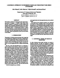
In some applications such as geophysics2{5 radioastronomy,6 radar7 or physico-chemical experiments,8 we may know that the input signal x(t) is the superposition (or a linear combination) of some known or unknown elementary signals gk (t), for example K X (4) x(t) = ak gk (t ? tk ): k=1
The problem then becomes estimating ak , tk and gk (t) (see Figure 1). g1(t) g2(t)
- D(t ) - D(t )
gK (t) -
rr
1
g1(t ? t1 ) -
a1
2
g2(t ? t2 ) -
a2
gK (t ? tk )-
aK
D(tK )
rr
�� ��
ZZ ZZ~- x(-t) ?� � ? ? ?
? �� ��b(t)
�
h(t)
y(t)
Figure 1: Data generation model. This data generation model arises in many remote sensing signal processing areas such as source separation9 (see Figure 2) and impulse input deconvolution10 (see Figure 3). s(t) 6 s1(t) s2(at) 62 a 1 6 t1
t2
6
sk (t) 6ak tk
rrr
s1 (t) = a1 � (t ? t1) -
sK (t) aK
6
tK
g1
rr
s2 (t) = a2 � (t ? t2) -
g2
-t sK (t) = aK �(t ? tK-)
gK
�� ��
ZZ ZZ~- x(-t) � ??� ??
�� ? ��b(t)
h(t)
�
y(t)
? �� ��-
Figure 2: Source separation model. s(t) =
K X k=1
ak � (t ? tk )
-
g(t)
x(t)
-
b(t)
h(t)
�
y(t)
Figure 3: Pulse input deconvolution model. However, most of the time gk (t) has a known (or assumed so) form with unknown parameters such as Gaussian, Lorentzian, Sinc, Sinusoidal, Exponential, etc. : � � ?t2 � � sin(2�sk t) ; sin(2�s t); exp [?j 2�s t] s2 gk (t) = exp (5) ; 2 k 2; k k 2sk sk + t (2�sk t) so that the deconvolution problem becomes that of estimating fak ; tk ; sk ; k = 1; � � � ; K g and K . The detection step consists in hypothesis testing of H0 : K = 0 against H1 : K 6= 0. By localization we mean the estimation of t = [t1; � � � ; tK ], by estimation we mean the determination of a = [a1; � � � ; aK ] and by source characterization we mean the estimation of s = [s1; � � � ; sK ].
We address exactly these problems here using a Bayesian approach and more speci cally the maximum a posteriori (MAP) estimation method. In a Bayesian estimation framework, the main idea is to assign prior probability laws to all of the unknowns and then combine them with the likelihood of the data to obtain the posterior law of those unknowns and naly de ne an estimator for them. In our case, this means that we can assign the probability distributions P (K = k) = p(k), p(ajK ), p(tjK ), p(sjK ), and p(yja; t; s; K ).
2 Proposed method Let us to rewrite the data generation model in a slightely di�erent way: y(t) = h(t) � x(t; a; t; s) + n(t)
with
x(t; a; t; s) =
K X k=1
ak gk (t ? tk ):
(6)
The problem becoming now the estimation of the parameters a; t; s; K . Classicaly, many authors assume K known and try to estimate the other ones by minimizing the Least Squares (LS) criterion, i.e. ( ) M X 1 2 (ab; bt; bs) = arg min Q(a; t; s) = 2M jy(ti ) ? h � x(ti; a; t; s)j (7) (a;t;s) i=1 This approach may not give satisfaction in many di�cult situations where the data are poor (either by their number or due to the noise). Also, in this approach, implicitly, a Gaussian distribution for the noise is assumed. What we propose is to give a more general approach which can also take account of prior knowledge (either soft and hard constraints) on the unknwon parameters and on the errors (modelling and the measurement noise). The Bayesian estimation approach is an appropriate framework for this task. If we assume that we can assign the probability laws P (K = k) = p(k), p(ajK ), p(tjK ), p(sjK ) and p(yja; t; s; K ) to translate our prior knowledge on the parameters K , a, t and s and on the errors, and if we assume that these parameters are a priori independant, then we can calculate the joint posterior law by applying the Bayes' rule: p(yja; t; s; K ) p(ajK ) p(tjK ) p(sjK ) P (K ) (8) p(a; t; s; K ) = p(y) where Z KX max p(y) = p(k) p(yja; t; s; k) p(ajk) p(tjk) p(sjk) da dt ds (9) k=0
From this joint posterior law, we can calculate any marginals: Z P (K = kjy) = p(a; t; s; kjy) da dt ds Z p(ajy; k) = p(k) p(a; t; sjy; k) dt ds Z p(tjy; k) = p(k) p(a; t; sjy; k) da ds Z p(sjy; k) = p(k) p(a; t; sjy; k) da dt
(10) (11) (12) (13)
We can then theoretically use them to make any inference about these parameters. For example, we can make detection by comparing the probabilities P (K 6= 0jy) and P (K = 0jy) or estimate any of the parameters � = fa; t; sg by �b = arg max fp(� jy; k)g with � = a; t; or s: (14) �
However, one of the main di�culties in this approach is the calculation of these integrals. What we propose here is to estimate jointly all the unknown parameters by (ab; bt; bs; Kb ) = arg max fp(a; t; s; kjy)g : (15) a;t;s;k)
(
Separating the discrete value parameter K from the real value parameters a, t and s and assigning an uniform prior for K in the range [0; Kmax ], will permit us to rewrite this solution as: (ab ; bt; bs) = arg min fJk (a; t; s)g (16) (a;t;s) n o (17) Kb = arg min Jk (ab ; bt; bs) k where
and
Jk (a; t; s) = Qk (a; t; s) + H1k (a) + H2k (t) + H3k (s);
(18)
Qk (a; t; s) = ? ln p(yja; t; s; K = k); H1k (a) = ? ln p(ajK = k); H2k (a) = ? ln p(tjK = k); H3k (a) = ? ln p(sjK = k):
(19) (20)
Now, we are going to discuss the appropriate choices of the prior laws for the noise andfor the unknwon parameters. It is very usual to assume that the noise is zero-mean, white and Gaussian with known variance �2: M 1 X 2 p(yja; t; s; k) = (2�)?M=2 �?M exp [?Qk (a; t; s)] with Qk (a; t; s) = 2 2� i=1 jy(ti ) ? h � x(ti ; a; t; s)j (21) We may also assume that all the ak , tk and sk have to be strictly positive. To ensure this constraint we can choose Gamma priors probabilities for them. This is not the unique possible choice. Any other probability distribution which is de ned on IR+ may be used. What we propose is to choose the following one parameter prior laws:
� The amplitudes ak > 0 are assumed to be mutually indepentant K Y p(ajK ) = pk (ak ); and follow the Gamma law
(22)
k=1
1 �?1 (23) ?(�) z exp [?z ] ; � > 0: This hypothesis insures the amplitudes to be positive and the parameter � controls their mean and variance. In fact, the mean and the variance of a random variable Z with this probability law are E fZ g = Var fZ g = �: (24) With this hypothesis, the expression of H1k (a) becomes K K X X H1k (a) = ? ln p(ajK ) = (1 ? �) log(ak ) + ak + K ln?(�) (25) pk (z ) =
k=1
k=1
� In the same way, the positions tk ? tk?1 > 0 are also assumed to be mutually independant and follow a Gamma law 1 z ?1 exp [?z ] ; > 0: (26) p(tk ? tk?1 = z ) = ?( )
Note that with this hypothesis tk > 0 constitute a rst order Markov chain and we can write: p(t) = p(t1 )
with
p(t1 ) =
and
K Y k=2
p(tk jtk?1);
(27)
1 ?1 ?( ) t1 exp [?t1] ; > 0;
1 ?1 ?( ) (tk ? tk?1) exp [?(tk ? tk?1)] ; With this hypothesis on tk the expression of H2k (t) becomes p(tk jtk?1) =
H2k (t) = ? ln p(tjK ) = (1 ? )
K X k=1
log(tk ? tk?1) +
K X k=1
(tk ? tk?1) + K ln ?( ); with t0 = 0:
(28) (29)
(30)
� The parameters sk > 0 (which are either the variances or the frequencies) are also assumed to be mutually independent
p(sjK ) =
and follow the Gamma prior
K Y k=1
pk (sk )
(31)
1 z ?1 exp [?z ] ; > 0: ?( ) With this hypothesis the expression of H3k (s) becomes pk (z ) =
H3k (s) = ? ln p(sjK ) = (1 ? )
K X k=1
log(sk ) +
K X k=1
sk + K ln ?( ):
(32)
(33)
Now, the main problem is how to optimize e�ectively the criterion J which may be multimodal. However, we can calculate analytically the gradient and the Hessian of the criterion. So, we propose the following alternatives: { either use local optimization scheme such as a gradient based iterative algorithm with a good initialization; { or try to use a global optimization such as simulated annealing or some deterministic relaxation schemes such as ICM (Iterated Conditional Modes)11 or ICD (Iterated Coordinate Descent).12,13 Note however that the local optimization needs a fair initialization to be in the attractive region of the global minimum of the criterion. For initialization, we propose rst to use a classical deconvolution (for example a Tikhonov regularization with positivity constraint) to nd a solution from which we can propose a good initialization. However, the simulations showed that the method is enough robust to this initialization.
3 Proposed algorithm The proposed algorithm is the following: 1. For K = 0 to Kmax Optimize JK (a; t; s) to obtain (ab; bt; bs)K and note the optimum value JKo End 2. Choose the Kb which gave the minimum value of the JKo .
For the optimization of JK (a; t; s) we use a modi ed Newton-Raphson algorithm applied separately to each set of parameters a, t and s which can be summarized as follows: � (n+1) = � (n) + ��(n) with � = a; t or s (34) and where h i?1 ��(n) = ?� D(n) r� J (� (n)); (35) and � @2J � @ 2 J (n) (n) (n) D = diag (� ); � � � ; 2 (� ): (36) @�1 2 @�m To go further in details of the implementation, note K X �y(ti ) = y(ti ) ? h � x(ti ) = y(ti ) ? [h � gk ](ti ? tk ): (37) k=1
Then we have the following relations: Q(a; t; s) =
and
�
M 1X 2 2 i=1 j�y(ti )j
(38)
�
M X @g @Q h � k (ti ? tk ) �y(ti ) = ? @�k @� k i=1 " � @g �2 # M X @2Q @ 2 gk (ti ? tk )�y(ti ) h� 2 ? h� k = ? @�k @�k 2 @�k i=1 with �k = ak ; tk or sk : The next step is to calculate the rst and second derivatives of g with respect to the parameters �k .h This dependsi of course on the special function gk . For exemple, in the case of gausian function gk (t ? tk ) = exp 2?s1k (t ? tk )2 ,
we have the following relations: @gk (t ? tk ) 1 @ 2 gk (t ? tk ) = gk (t ? tk ) =0 @ak ak @ak 2 2 @gk (t ? tk ) (t ? tk ) @ gk (t ? tk ) ?sk + (t ? tk )2 = = gk (t ? tk ) and gk (t ? tk ) @tk sk s2k @tk 2 2 2 2 2 @gk (t ? tk ) (t ? tk ) @ gk (t ? tk ) ?4sk (t ? tk ) + (t ? tk )4 = g ( t ? t ) = gk (t ? tk ) k k @sk 2s2k @sk 2 4s4k Finally, we need to calculate the gradients of H1(a), H2(t) and H3(s) : @H1 1 ? � @ 2 H1 ?(1 ? �) = +1 = @ak ak 1? +1 @H2 = @tk tk ? tk?1 @H3 ?1 = s +1 @sk k
and
@ak 2 a2k ? (1 ? ) @ 2 H2 = 2 (tk ? tk?1)2 @tk @ 2 H3 1 = @sk 2 s2k
Now, we have all the ingredients to calculate the gradient r� J (�) and the matrix D to implement the proposed algorithm. To reduce the computation burden and to implement the algorithme e�ciently, we can remark that we need the following calculations: gk (t), z (t) = [h � x](t), uk (t) = [tgk](t), vk (t) = [t2gk ](t), wk (t) = [t4gk ](t), [h � gk ](t), [h � uk ](t), [h � vk ](t), [h � wk ](t) which lead us to the calculation of �y(t), the gradient of the criterion and the diagonal elements of its Hessian matrix.
4 Simulations To show the performances of the proposed method we simulated an input signal x(t) with the following parameters: a = [1; 2; 1:4; 0:7]; t = [200; 250; 300; 350]; s = [10; 15; 20; 10]; an impulse response h(t) and calculated [h � x](t) and added a Gaussian noise to obtain y(t) with a signal to noise ratio SNR=20dB. (Figure 4). In this gure we can also see the results that can be obtained with classical deconvolution methods such as Wiener ltering, regularization with a quadratic functional and regularization with an entropic functional. 2.5
2.5
2 2
1.5 1.5
1
1 0.5
a)
0.5
0
0
50
100
150
200
250
300
350
400
450
500
2.5
g)
0
−0.5
0
50
100
150
200
250
300
350
400
450
500
0
50
100
150
200
250
300
350
400
450
500
−0.5 0
50
100
150
200
250
300
350
400
450
500
50
100
150
200
250
300
350
400
450
500
50
100
150
200
250
300
350
400
450
500
2.5
2 2
1.5 1.5
1
1 0.5
b)
0.5
0
0
50
100
150
200
250
300
350
400
450
500
0
50
100
150
200
250
300
350
400
450
500
2.5
h)
0
−0.5
2
1.5
1
c)
0.5
0
2.5
2.5
2 2
1.5 1.5
1 1
0.5
d)
0.5
0
0
50
100
150
200
250
300
350
400
450
500
2.5
i)
0
2.5
2 2
1.5 1.5
1 1
0.5
e)
0.5
0
0
50
100
150
200
250
300
350
400
450
500
j)
0
−0.5 0
2.5
2
0.02
1.5 0.015
1 0.01
0.5
f)
0.005
0
50
100
150
200
250
300
350
400
450
500
k)
0
−0.5 0
Figure 4: Di�erent steps of data construction and the results obtained by direct deconvolution: a,b,c,d,e,f) g1(t); g2(t); g3(t); g4 (t); x(t) and h(t); g,h) y(t) without and with noise, i,j,k) Results of deconvolution by: i) Wiener ltering, j) Regularization with a quadratique regularization term,w k) Regularization with an entropic regularization term. Figure 5 shows the di�erent steps of the proposed algorithm: At each step (for di�erent values of K from 0 to Kmax we show the initialization (which is obtained from the results obtained in the previous step and a new component initialized using also the residual in the previous step), the nal estimate and the criterion evolution during the iterations.
a
2
b
3
c
4
2.5
x 10
1.8 2.5 1.6
1.4 2
2
1.2
1
1.5
0.8 1
1.5
0.6
0.4 0.5
k=1
0.2
0
0
50
100
150
200
250
300
350
400
450
500
3
0
0
50
100
150
200
250
300
350
400
450
500
2.5
1
0
5
10
15
20
25
30
35
40
7000
6500
2.5 2
6000 2 1.5 5500 1.5 5000 1 1 4500 0.5 0.5
k=2
0
4000
0
50
100
150
200
250
300
350
400
450
500
0
2.5
2.5
2
2
1.5
1.5
1
1
0.5
0.5
0
50
100
150
200
250
300
350
400
450
500
3500
0
5
10
15
20
25
30
35
40
0
5
10
15
20
25
30
35
40
0
5
10
15
20
25
30
35
40
0
5
10
15
20
25
30
35
40
0
5
10
15
20
25
30
35
40
2500
2400
2300
2200
2100
2000
1900
k=3
1800
1700
0
0
50
100
150
200
250
300
350
400
450
500
0
0
2.5
2.5
2
2
1.5
1.5
1
1
0.5
0.5
50
100
150
200
250
300
350
400
450
500
1600
2600
2500
2400
2300
2200
2100
2000
1900
k=4
1800
1700
0
0
50
100
150
200
250
300
350
400
450
500
2.5
2
0
0
50
100
150
200
250
300
350
400
450
500
1600
2
3600
1.8
3400
1.6
3200
1.4 3000 1.5
1.2 2800 1 2600
1
0.8 2400 0.6
0.5
k=5
k=6
2200
0.4
2000
0.2
0
0
50
100
150
200
250
300
350
400
450
500
0
0
50
100
150
200
250
300
350
400
450
500
1800
2
2
4200
1.8
1.8
4000
1.6
1.6
3800
1.4
1.4
3600
1.2
1.2
3400
1
1
3200
0.8
0.8
3000
0.6
0.6
2800
0.4
0.4
2600
0.2
0.2
0
0
50
100
150
200
250
300
350
400
450
500
0
2400
0
50
100
150
200
250
300
350
400
450
500
2200
Figure 5: Signal separation results for k = 1; � � � ; 6. a) Initialization in each step obtained from the results in its previous step and a new component; b) Final result in each step; c) Evolution of the criterion during the iterations.
To be ensured that the proposed algorithm works well in other situations, we simulated two other cases: the rst one with K = 4 and the other with K = 5. In each case we added a new component at one side or at the other. Figure 6 shows the model selection criterion JK in fonction of K in the three cases K = 3, K = 4 and K = 5. We can remark that the optimum in each case corresponds to the correct value. K =3
K=4
8000
K=5
12000
18000
16000
7000
10000 14000
6000 8000
12000
5000
10000
6000 8000
4000
6000
4000 3000
4000
2000
2000
2000
1000
1
1.5
2
2.5
3
3.5
4
4.5
5
5.5
0
6
0
1
1.5
2
2.5
3
3.5
4
4.5
5
5.5
6
2.5
2.5
2.5
2
2
2
1.5
1.5
1.5
1
1
1
0.5
0.5
0.5
0
0
50
100
150
200
250
300
350
400
450
500
0
0
50
100
150
200
250
300
350
400
450
500
0
0
2.5
2.5
2.5
2
2
2
1.5
1.5
1.5
1
1
1
0.5
0.5
0.5
0
0
0
−0.5
0
50
100
150
200
250
300
350
400
450
500
−0.5
0
50
100
150
200
250
300
350
400
450
500
−0.5
2.5
2.5
2
2
1.5
1.5
1.2
1
1
0.8
0.5
0.5
1
1.5
50
0
50
2
100
100
2.5
150
150
3
200
200
3.5
250
250
4
5
5.5
350
400
450
500
300
350
400
450
500
300
350
400
450
500
300
4.5
6
2
1.8
1.6
1.4
1
0.6
0.4
0.2
0
0
50
100
150
200
250
300
350
400
450
500
0
0
0
50
100
150
200
250
300
350
400
450
500
0
50
100
150
200
250
Figure 6: Model selection criterion a) Model selection criterion JK in fonction of K , b) Original signals; c) data and d) recostructed signals in each case.
5 Conclusions We presented a Bayesian aproach to detection, localization and characterization (estimation of signal components parameters) from a limited number of noisy data. The Bayesian estimation framework to solve these inverse problems lets us easily to account of prior information on the unknown parameters, and by this way, helps us to nd satisfacory results to theses ill-posed or ill-conditionned problems. In this paper we proposed to use the maximum a posteriori (MAP) estimation method with some speci c choices for the prior laws and we presented some algorithmes to handle with the resulted optimization problems. The simulations seem to give satisfactory results in di�erent situations.
6 REFERENCES [1] G. Demoment, \Image reconstruction and restoration : Overview of common estimation structure and problems," IEEE Transactions on Acoustics Speech and Signal Processing, vol. ASSP-37, pp. 2024{2036, December1989. [2] J. Bednar, R. Yarlagadda, and T. Watt, \L-1 deconvolution and its application to seismic signal processing," IEEE Transactions on Acoustics Speech and Signal Processing, vol. ASSP-34, no. 6, p. 1655, 1986. [3] H. Chuberre and J. Fuchs, \A deconvolution approach to source localization," in Proceedings of IEEE ICASSP, pp. 253{256, avril1993. [4] H. El-Sherief, \Adaptive least squares for parametric spectral estimation and its application to pulse estimation and deconvolution of seismic data," IEEE Transactions on Systems, Man and Cybernetics, vol. SMC-16, pp. 299{303, 1986. [5] J. Goutsias and J. M. Mendel, \Maximum-likelihood deconvolution : An optimization theory perspective," Geophysics, vol. 51, pp. 1206{1220, 1986. [6] Schultz, \Multiframe blind deconvolution of astronomical images," Journal of the Optical Society of America, vol. 10, May1993. [7] Holmes, \Blind deconvolution of quantum-limited incoherent imagery : Maximum-likelihood approach," Journal of the Optical Society of America, vol. 9, July1993. [8] A. Kumar, C. Sotak, C. duMoulin, and G. Levy, \Software for deconvolution of overlapping spectral peaks and quantitative analysis by 13c fourier transform NMR spectroscopy," Comput. Enhanced Spectrosc. (GB), vol. 1, pp. 107{114, Apr. 1983. [9] K. Cheung and S. Yau, \Blind deconvolution of system with unknown response excited by cyclostationary impulses," in Proceedings of IEEE ICASSP, vol. 3, (Detroit, Michigan), pp. 1984{1987, mai1995. [10] F. Champagnat, Y. Goussard, and J. Idier, \Unsupervised deconvolution of sparse spike trains using stochastic approximation," IEEE Transactions on Signal Processing, vol. 44, pp. 2988{2998, d�ecembre1996. [11] J. E. Besag, \On the statistical analysis of dirty pictures (with discussion)," Journal of the Royal Statistical Society B, vol. 48, no. 3, pp. 259{302, 1986. [12] K. Sauer and C. Bouman, \A local update strategy for iterative reconstruction from projections," IEEE Transactions on Signal Processing, vol. SP-41, pp. 534{548, February1993. [13] S. Saquib, J. Zheng, C. A. Bouman, and K. D. Sauer, \Provably convergent coordinate descent in statistical tomographic reconstruction," in Proceedings of IEEE ICIP, vol. 2, (Lausanne, Switzerlande), pp. 741{745, septembre1996.