3-D Automatic Mesh Adaptation for Turbulent Flows ...... It occurs when the four points forming any one face on the element are no longer ..... (bottom) shows two adjoining tetrahedral elements with a swap of one of the internaI edges. 39 ...
NOTE TO USERS
This reproduction is the best copy available.
®
UMI
3-D Automatic Mesh Adaptation for Turbulent Flows Irmgard Frances Suerich-Gulick
A Thesis in the Department of Mechanical Engineering
Presented in Partial Fulfillment of the Requirements for the Degree of Master' s Thesis at McGill University Montréal, Québec, Canada
©France Suerich-Gulick, 2005
1+1
Library and Archives Canada
Bibliothèque et Archives Canada
Published Heritage Branch
Direction du Patrimoine de l'édition
395 Wellington Street Ottawa ON K1A ON4 Canada
395, rue Wellington Ottawa ON K1A ON4 Canada Your file Votre référence ISBN: 0-494-12653-1 Our file Notre référence ISBN: 0-494-12653-1
NOTICE: The author has granted a nonexclusive license allowing Library and Archives Canada to reproduce, publish, archive, preserve, conserve, communicate to the public by telecommunication or on the Internet, loan, distribute and sell th es es worldwide, for commercial or noncommercial purposes, in microform, paper, electronic and/or any other formats.
AVIS: L'auteur a accordé une licence non exclusive permettant à la Bibliothèque et Archives Canada de reproduire, publier, archiver, sauvegarder, conserver, transmettre au public par télécommunication ou par l'Internet, prêter, distribuer et vendre des thèses partout dans le monde, à des fins commerciales ou autres, sur support microforme, papier, électronique et/ou autres formats.
The author retains copyright ownership and moral rights in this thesis. Neither the thesis nor substantial extracts from it may be printed or otherwise reproduced without the author's permission.
L'auteur conserve la propriété du droit d'auteur et des droits moraux qui protège cette thèse. Ni la thèse ni des extraits substantiels de celle-ci ne doivent être imprimés ou autrement reproduits sans son autorisation.
ln compliance with the Canadian Privacy Act some supporting forms may have been removed from this thesis.
Conformément à la loi canadienne sur la protection de la vie privée, quelques formulaires secondaires ont été enlevés de cette thèse.
While these forms may be included in the document page count, their removal does not represent any loss of content from the thesis.
Bien que ces formulaires aient inclus dans la pagination, il n'y aura aucun contenu manquant.
•••
Canada
Acknowledgements 1 would like to thank my supervisor, Professor W.G. Habashi, for his guidance and for providing me with a stimulating and challenging work environment during the past years at the CFD Laboratory and at NT!. 1 am grateful to him for giving me the benefit of the doubt three and a half years ago when 1 was in a difficult situation and was in dire need of a supervisor for my Honour' s thesis. 1 also appreciate the financial support he provided me during a portion of my studies. 1 am extreme1y grateful to Dr. Claude Lepage, who provided me with guidance and support through aIl my time at the CFD Lab and NT!. He also contributed ideas and extensive editing to the writing of my thesis, without which this work would have been of lesser quality. 1 would also like to thank Dr. François Morency and Dr. Frédéric Tremblay for their advice on turbulence modeling, as weIl as Dr. Lakhdar Remaki for answering many questions about numerical schemes and strategies. 1 am grateful to everyone else at the CFD Lab and NT!, and in particular my fellow graduate students, Hong Zhi Wang, Raimund Honsek, Peter Findlay and Nabil Ben Abdallah, who made working at the Lab fun and who helped me get through difficult times. 1 would like to thank my boyfriend Jesse Olszynko-Gryn, for his companionship and support in innumerable ways through the past three years. Finally, 1 would like to thank my parents for loving me, for pushing me and encouraging me every step of the way. 1 would finally like to acknowledge the financial support that was provided to me by the National Sciences and Engineering Research Council of Canada, the Fonds québécois de la recherche sur la nature et les technologies, and the NSERC-J. Armand Bombardier Industrial Research Chair in Multi-disciplinary CFD at McGill.
11
To my mother, Hannelore Suerich-Storm 1941-2004
111
Abstract Computational fluid dynamics is increasingly used as an analysis and simulation tool in research and industry. Mesh generation remains a major challenge, in particular for turbulent flow simulations, as it can be very difficult and time-consuming to produce a good mesh that will produce accurate results. Mesh adaptation schemes have been developed to help improve the solutions obtained and facilitate the mesh generation process. This work expands the y+ correction scheme within an existing 3-D anisotropie mesh adaptation module for turbulent flow simulations developed at the McGill CFD Lab. First, the y+ correction scheme is improved for structured layers of elements when the turbulence model uses wall functions. Second, y+ correction is expanded to handle unstructured meshes that are more appropriate for complex geometries. Test cases are performed to evaluate the impact of the new y+ correction on the accuracy of the flow solutions.
IV
Résumé La simulation numérique de la dynamique des fluides est utilisée de plus en plus comme outil d'analyse et de simulation en recherche et en industrie. La génération de maillages demeure un défi majeur, en particulier pour la simulation d'écoulements turbulents, car il peut être très difficile et coûteux en temps de générer un maillage qui produira des résultats précis. Des schémas d'adaptation de maillages ont été développés pour contribuer à l'amélioration des résultats obtenus et pour faciliter le processus de génération de maillages. Ce travail poursuit le développement d'un schéma qui fait la correction d'T à l'intérieur d'un logiciel d'adaptation de maillages tridimensionnels développé au laboratoire de CFD de McGill, pour fins de simulations d'écoulements turbulents. D'abord, le schéma de correction d'Y+ pour les couches d'éléments structurés est amélioré, pour les cas où des fonctions de paroi sont utilisées par le modèle de turbulence. Ensuite, la mise en oeuvre du schéma de correction d'Y+ est élargie pour pouvoir traiter les maillages non-structurés, qui sont plus appropriés pour les géométries complexes. Des tests de validation sont déployés pour évaluer l'impact des nouvelles fonctions de correction d'T sur la précision des simulations.
v
Table of Contents List of Figures .................................................................................................................... ix List of Variab les ............................................................................................................. xiii
1
2
Introduction ................................................................................................................ 1 1.1
Motivation ............................................................................................................ 1
1.2
Literature Review .................................................................................................. 3
1.2.1
Turbulence Model Mesh Requirements in the Near-Wall Region ............. .4
1.2.2
y+ Correction Embedded in Mesh Adaptation ............................................ 5
1.2.2.1
y+ Correction of Structured Layers of Elements ..................................... 6
1.2.2.2
Boundary Layer Correction ofUnstructured Meshes .............................. 7
1.3
Thesis Objective and Scope ................................................................................. 8
1.4
Thesis Outline ...................................................................................................... 9
Turbulence Modeling............................................................................................... 11 2.1
General Properties of Turbulent Flow ............................................................... 11
2.2
Equations of Motion for Turbulent Flow ........................................................... 13
2.3
Turbulent Boundary Layer ................................................................................. 14
2.4
Turbulent Viscosity Models ............................................................................... 16
2.4.1
The k-e Model ............................................................................................ 18
2.4.1.1
3
Near-Wall Treatments ............................................................................ 19
2.4.2
Spalart-Allmaras Model ............................................................................. 21
2.4.3
Mesh Requirements of Turbulence Models ............................................... 23
Mesh Generation and Adaptation .......................................................................... 24
3.1
Characteristics of a Good Mesh for CFD .......................................................... 24
3.2
Mesh Types ........................................................................................................ 27
3.2.1
Hexahedral Block-Structured Meshes ....................................................... 28
3.2.2
Tetrahedral Unstructured Meshes .............................................................. 30
3.2.3
Hybrid Tetrahedra-Prism Mesh ................................................................. 32
3.3
Mesh Adaptation ................................................................................................ 34
3.3.1 3.3.1.1
Governing Princip les ................................................................................. 36 The Solution-Adaptation Cycle ............................................................. 37
Vl
3.3.1.2
Error Metric ........................................................................................... 38
3.3.1.3
Adaptation Operations ........................................................................... 39
3.3.1.4
Quality Metrics ...................................................................................... 40
3.3.1.5
Conserving and Improving Boundary Definition ................................. .41 y+ Correction for Turbulent Flows ............................................................ 42
3.3.2 3.3.2.1
Improving and Expanding y+ Correction .................................................. 45
3.3.3
4
Improving y+ Correction for Structured Layers of Elements ............................47 4.1
Transition Detection ........................................................................................... 47
4.1.1
Wall Functions and Transition Zones ....................................................... .48
4.1.2
Methodology .............................................................................................. 51
4.2
5
6
Methodology for Structured Layers ...................................................... .43
Improving Mesh Quality at Sharp Corners ........................................................ 56
y+ Correction For Unstructured Meshes ............................................................... 60
5.1
Desired Mesh Characteristics ............................................................................ 60
5.2
Methodology ...................................................................................................... 61
5.2.1
Computing the Distance from the Wall ..................................................... 62
5.2.2
Evaluating the Local Element Thickness ................................................... 64
5.2.3
Modifying the Metric ................................................................................. 64
5.3
Comparison with Other Schemes ....................................................................... 66
5.4
Additional Challenges ........................................................................................ 68
5.4.1
Preventing the Creation of 'Flat' Tetrahedra ............................................. 69
5.4.2
Computing a Local Minimum Aspect Ratio Constraint ............................ 73
Results ....................................................................................................................... 76 6.1
Flat Plate ............................................................................................................ 76
6.1.1
Geometry .................................................................................................... 77
6.1.2
Laminar Boundary Layer ........................................................................... 77
6.1.2.1
Flow Parameters ..................................................................................... 78
6.1.2.2
Mesh Configurations .............................................................................. 78
6.1.2.3
Discussion ofthe Flow Solutions .......................................................... 81
6.1.3 6.1.3.1
Turbulent Boundary Layer ......................................................................... 85 Geometry and Flow Parameters ............................................................. 85
vu
6.2
7
6.1.3.2
Computational Meshes ........................................................................... 86
6.1.3.3
Discussion ofthe Flow Solution ............................................................ 88
NACA-0012 Wing at 10° AoA, Turbulent Subsonic Flow ............................... 93 6.2.1.1
Geometry................................................................................................ 93
6.2.1.2
Flow Parameters ..................................................................................... 94
6.2.1.3
Computational Meshes ........................................................................... 94
6.2.1.4
Discussion of Computed Solutions ........................................................ 99
6.3
Mesh Pre-Processing on a High-Lift Wing ...................................................... 101
6.4
Hybrid Mesh Pre-processing on a Boeing 737-300 Nacelle Model ............... l02
Conclusions ............................................................................................................. 104
7.1
Contributions.................................................................................................... 104
7.2
Future Work ..................................................................................................... 107
References ....................................................................................................................... 109
Vlll
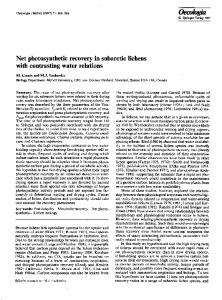
List of Figures Figure 1 - Different regions of the turbulent boundary layer profile ............................... 15 Figure 2 - Standard 3-D elements ................................................................................... 25 Figure 3 - Examp1e of a skewed quadrangle (left) and warped hexahedron (right) ........ 27 Figure 4 - Hexahedral mesh adapted to align the mesh with an oblique shock............... 27 Figure 5 - Example of three mesh types at the leading edge of an airfoil: structured mesh (left), unstructured mesh (centre) and hybrid mesh (right) .............. 28 Figure 6 - Example of a structured blocking (left) and mesh (right) around a turbine blade ............................................................................................................................ 29 Figure 7 - Hybrid meshes: a column ofthree layers ofprisms extruded from a triangular surface mesh (left) and a section through a mesh at the leading edge of an airfoil (right) ........................................................................................................... 33 Figure 8 - Deformed prism elements at the trailing edge ofa NACA-0012 airfoil.. ....... 34 Figure 9 - Flow chart of the CFD process with mesh adaptation pre-processing............ 37 Figure 10 - Edge operations: one tetrahedron is split in two (top), the middle ofthree tetrahedra is collapsed (centre), and the edge between two tetrahedra is swapped (bottom) ....................................................................................................................... 40 Figure Il - Initial mesh (left), adapted mesh without CAD projection (centre) and adapted mesh with CAD projection (right) ................................................................. 42 Figure 12 - Side view of a typical hybrid mesh configuration with y+ correction variables ...................................................................................................................... 43 Figure 13 - Diagram of structured layers of elements being adjusted in height and aligned perpendicular to the wall ................................................................................ 44 Figure 14 - Detail ofhybrid mesh at the trailing edge of a wing: initial mesh (left), pre-processed mesh with aligned normals (right) ....................................................... 45 Figure 15 - Example of deformed elements generated by y+ correction at the stagnation point on a NACA-0012 wing at 10° AoA. Original mesh (top left), Mach Number contours (top right), y+ distribution on the surface (bottom left), and adapted mesh with y+ correction with Y\arget = 40 (bottom right) ...................... 48 Figure 16 - Reichardt's velocity profile for a fully turbulent boundary layer ................. 50
IX
Figure 17 - Velocity profiles at different locations along the chord of a NACA-0012 airfoil, compared to Reichardt's profile ...................................................................... 52 Figure 18 - 2-D ex ample ofthe computation ofutan ........................................................ 53 Figure 19 - Leading edge ofNACA-0012 at 10° AoA. Mach number contours (top left), smoothed transition coefficient a on the wall (top right). Adapted meshes with y+ correction (bottom), without transition detection (left) and with transition detection (right) ........................................................................................................... 55 Figure 20 - Mesh detail at the trailing edge of a wing: initial mesh (left), adapted mesh with adjusted element height and aligned norma1(right) ................................... 56 Figure 21 - Velo city vectors on a mesh with aligned normal edges at the trailing edge ofa NACA-0012 wing at 10° AoA ............................................................................. 57 Figure 22 - 2-D view oftwo surfaces meeting at a sharp corner..................................... 58 Figure 23 - Computation of the slanted vector in a column of prisms near a sharp corner........................................................................................................................... 59 Figure 24 - Modification of edge alignment: initial mesh (left), pre-processed mesh with perpendicular normals (right), pre-processed mesh with slanted normals ......... 59 Figure 25 - Side view of a typical unstructured mesh with y+ correction variables ....... 61 Figure 26 - Computing the distance to the nearest wall node ......................................... 63 Figure 27 - Normal distance dproj computed by projecting on the normal of the face adjoining the nearest wall node ................................................................................... 64 Figure 28 - 2-D example of the computation ofthe new eigenvectors Vnonn and Vn .... 65 Figure 29 - Irregularly refined surface mesh produced by mesh adaptation when the adaptation process is too constrained .......................................................................... 69 Figure 30 - Two different tetrahedral element shapes commonly produced by the adaptation: 'flat' tetrahedra (left) and pyramid-shaped tetrahedra (right) .................. 70 Figure 31 - 2-D example ofthe maximum dihedral angle of a triangular element. ........ 70 Figure 32 - Circumscribed sphere about a flat tetrahedron (left) and a pyramid-shaped tetrahedron (right) ....................................................................................................... 71 Figure 33 - Pre-processed mesh on the surface and on the symmetry plane with the improved aspect ratio formula .................................................................................... 72
x
Figure 34 - Detail ofleading edge (left) and trailing edge(right) ofNACA-0012 wing with locked elements near the curved wall and the sharp corner................................ 74 Figure 35 - Detail ofpre-processed mesh with ARmin,local at the leading edge (left) and trailing edge (right) ofthe NACA-0012 wing ............................................................. 75 Figure 36 - Detail views ofmeshes for laminar case at xlL = 0.0 (left) and xlL = 1.0 (right), from top to bottom: structured mesh, initial unstructured mesh, pre-processed unstructured mesh, adapted unstructured mesh ................................... 80 Figure 37 - Velo city contours at the leading edge ofthe laminar flat plate on the structured mesh (top), on the pre-processed unstructured mesh (middle) and on the adapted unstructured mesh (bottom) ........................................................................... 81 Figure 38 - Ve10city profile at xlL = 1.0 obtained with the different meshes .................. 82 Figure 39 - Cf obtained on the unstructured meshes, compared to Blasius' solution ...... 83 Figure 40 - Convergence of adaptation-solution cycles for unstructured mesh when pre-processing is not employed (velocity profile at x/L = 1.0)................................... 84 Figure 41 - Detail views ofmeshes for turbulent case atxlL = 0.0 (left) and x/L = 1.0 (right), from top to bottom: structured mesh, initial unstructured mesh, pre-processed unstructured mesh, adapted unstructured mesh ................................... 87 Figure 42 - Velo city profile at x = L obtained on the structured mesh with 2nd order artificial viscosity and eAY = 1.98 x 10⁴ ..................................................................... 88 Figure 43 - Velocity profile at x = L obtained on the adapted unstructured mesh and the structured mesh (linear scale for d at top and logarithmic scale at bottom) ... 90 Figure 44 - Comparison of the velocity profile obtained with different levels of artificial Yiscosity on the adapted unstructured mesh ................................................. 91 Figure 45 - Comparison of Cf obtained on the different meshes (top) and with different levels of eAY (bottom) ................................................................................... 92 Figure 46 - Structured mesh for the NACA-0012 wing .................................................. 95 Figure 47 - Initial isotropie unstructured mesh (top) and pre-processed unstructured mesh (bottom) on the symmetry plane ........................................................................ 96 Figure 48 - Detail ofleading edge ofNACA-0012 wing: structured mesh (left), initial unstructured mesh (middle) and pre-processed unstructured mesh (right) ................. 96
Xl
Figure 49 - Solution-based adapted mesh without y+ correction (top) and with y+ correction (bottom) ...................................................................................................... 97 Figure 50 - Detail of the mesh near the leading edge, from left to right: initial mesh, pre-processed mesh, adapted mesh with y+ correction, adapted mesh without y+ correction..................................................................................................................... 98 Figure 51 - Mach number contours of the solution obtained on the initial unstructured mesh (top) and the pre-processed unstructured mesh (bottom) .................................. 99 Figure 52 - Comparison of Cp on the different meshes ................................................... 100 Figure 53 - Symmetry plane of the initial mesh (top) and pre-processed mesh on the high-lift wing ............................................................................................................... l 01 Figure 54 -Detail views of the initial mesh (top) and pre-processed mesh (bottom) on the high-lift wing: slat (left) and junction between main section and flap (right) ...... 102 Figure 55 - Nacelle, initial hybrid mesh (left) and pre-processed hybrid mesh (right) with y+ correction in the structured layers and the unstructured elements ................. 103 Figure 56 - Detail of symmetry plane mesh for the nacelle: initial mesh (left) and preprocessed mesh (right) ................................................................................................ 103
Xll
List of Variables a
element thickness growth ratio
a
transition flag coefficient
AR
aspect ratio
ARmin
minimum mesh aspect ratio
ARmin,tetra
minimum tetrahedral aspect ratio
ARmin,local
local minimum mesh aspect ratio
c
wing chord length coefficient of friction coefficient of pressure distance to the nearest wall vector pointing from wall node Wj to volume node vnodei boundary layer thickness error along an edge coefficient of artificial viscosity
h
local element thickness
H
Hessian matrix
K
von Karman' s constant
L
characteristic length of the flow
lmin
length of the shortest edge of an element
lmax
length of the longest edge of an element
Â.i
eigenvalue of the Hessian
A
diagonal matrix of the eigenvalues of the Hessian
M
Machnumber
N
number of layers of elements selected for y+ correction
n
normal to the wall dynamic viscosity of the fluid
v
kinematic viscosity of the fluid turbulent viscosity of the flow radius of curvature of the wall surface
X1l1
Re
Reynolds number radius ofthe sphere inscribed within a tetrahedral element radius ofthe sphere circumscribed about a tetrahedral element
p
density of the fluid shear stress at the wall
u
local mean flow velo city
if
non-dimensional velocity free-stream velocity
U
local velocity vector
Utan
component ofthe velocity vector that lies tangent to the wall friction velocity at the wall eigenvector of the Hessian
v
matrix of the three eigenvectors of the Hessian
v
vector detining an element edge
X
location of a point in space
y+
non-dimensional distance from a no-slip wall
Y max
upper limit ofY+ correction, in terms ofphysical distance
Y+max
upper limit ofY+ correction, in terms ofY+
y+ target
target y+ value for the tirst node away from the wall
y +sol
local y+ value from the flow solution target thickness of tirst element at the wall
Yl,metric
target element thickness at wall, computed based on the metric
Yl,Y+
target element thickness at the wall, computed based on Y+target
Ytop
target height of the top node of the structured layers of elements
XIV
1
Introduction
1.1
Motivation
For many fluid applications involving complex flows and geometries, Computational Fluid Dynamics (CFD) is increasingly able to pro duce accurate results in a cost-effective way. It is used as a design and analysis tool in both the research and industrial arenas, ranging from manufacturing processes to biomechanics to the aerospace industry. In many instances, CFD has replaced physical models in research and development, as it is capable of providing more detailed results than experimental techniques, and often at a significantly lower co st. CFD is by no means a complete and perfect tool and it is the object of much research both in academic and industrial settings. Indeed, several types of flows and geometries continue to pose a challenge for CFD simulation, either in terms of the level of accuracy that can be attained, or the amount of time and computing power required to perform the simulation. The quality of results is also strongly dependent on the user' s level of training and experience and on the assumptions that are made when setting up the simulation. The mean flow is described by the Navier-Stokes equations and the effect of turbulence on the mean flow is described using a turbulence mode!. These equations are non-linear and coupled, so theyare solved numerically for a given geometry and set of boundary conditions. Numerical solution is achieved by discretizing the domain and the equations so that the solution can be approximated with discrete analytical functions over sub-sections of the domain. The discretized domain is referred to as the mesh, which is generated using a number of different techniques. There are also different methods used to discretize the equations. The fini te volume method is commonly used in commercial flow solvers. For the test cases in this work, the finite element method based on the weak-Galerkin formulation is employed in the flow solver. This formulation uses linear shape functions to approximate the variation and the gradients of the different variables across each mesh element. In regions where the flow gradients change quickly, the linear shape functions cannot perfectly match the continuous shape of the 'exact' solution, and the discretization error is proportional to the
1
size of the mesh elements and the degree of curvature in the solution. The error also increases if the elements are too severely deformed. Different approaches can be used to improve the numerical solution by reducing the error associated with the discretization. One approach is to modify the discretization scheme for the equations, for example by using higher order shape functions. This requires the use of higher order elements, so both the mesh and flow solver must be changed. Another approach is to increase the density of the mesh in regions of high curvature in the flow and geometry. This allows the solution to be improved without the added complexity of higher order elements, and is applicable to almost any type of solver discretization. Mesh adaptation uses this approach. There are many hurdles to cost-effective and accurate simulations in CFD, among which are mesh generation and turbulence modeling. Mesh generation can be very difficult and extremely time-consuming for complex geometries and can represent up to 80% of the time spent by engineers to obtain a CFD solution [1]. It is challenging because there are many constraints regarding the properties of a good mesh. The mesh must have a high enough resolution to capture key flow features (which may not be known a priori) and must conform to the boundary of the flow domain. At the same time, the size of the mesh is limited by computing and memory resources. Even if the user knows what mesh density is desired at a specific location, it is sometimes difficult to achieve the desired node distribution and element connectivity. Different techniques have been proposed to improve mesh quality while reducing the amount of effort required on the part of engineers to produce the mesh and make the flow solution it generates 'userindependent'. For example, the mesh generation process for structured meshes can be substantially accelerated if many of the geometries to be meshed consist of variations of the same basic configuration. Then a grid topology can be developed for one configuration and modified to generate the meshes for different variations of that configuration. Mesh generation is further complicated by the needs of turbulence models. Turbulent flow is inherently unsteady and is characterized by the random motion of the fluid partic1es, which experience velo city fluctuations over a wide range of time and length scales. To simulate the full range of the turbulent flow behavior requires excessively
2
small element sizes and time steps that are not viable for industrial-scale applications. A variety of turbulence models are therefore employed to predict the mean effect of the turbulent fluctuations on the flow without computing the full range of turbulent motion. The most commonly used class of models is the RANS (Reynolds-Averaged NavierStokes) turbulence models. These models perform reasonably well under the specifie conditions for which they were designed, but have specifie requirements regarding the mesh density and configuration, particularly in the boundary layer region. These additional constraints bring new challenges to the task of generating the mesh and sometimes cannot be fully satisfied using standard mesh generation software. Mesh adaptation has proved to be a use fui tool that can help achieve improved solutions for inviscid and viscous flow simulation at a reduced cost, and it is regarded as a necessary and standard component of CFD by many researchers. Mesh adaptation operates on an initial mesh that has been generated using standard mesh generation software and on which an initial solution has been obtained. The mesh adaptation module estimates the error of the initial solution and modifies the mesh to minimize or to equalize the estimated error over the entire mesh. The resulting adapted mesh is tailored to the flow solution and thus allows a better solution to be obtained at the lowest cost. This can save the user time spent in generating the initial mesh, as well as reduce and ideally eliminate the need to regenerate the mesh several times in an effort to obtain first a converging solution and then a sufficiently accurate one. In order to extend the usefulness of mesh adaptation to turbulent flow simulations, the special requirements of the turbulence models must be incorporated into the mesh adaptation module. This work seeks to contribute to the incremental development of CFD as a useful tool for turbulent flow simulations by developing and testing specialized treatment of the mesh in boundary layer regions within an existing mesh adaptation module so that the adapted meshes correspond better to the needs of the turbulence models.
1.2
Literature Review
A brief review of the scientific literature is performed, first regarding the importance of the mesh in turbulent flow solutions, and second to see how researchers have modified their mesh generation and adaptation modules to account for the needs of turbulence
3
models. This second portion of the literature review shows what has been done in the past, and serves as inspiration for the new developments presented in this thesis. The review reveals discussion of the effect of near-wall mesh density on the quality of turbulent flow solutions obtained with RANS turbulence models in a few papers, and a few researchers note cases where there is a significant effect on the solution when the element thickness in the boundary layer is varied [2-3]. These findings are described below. Sorne researchers have incorporated special boundary layer correction into existing mesh adaptation modules [4-7] and a few have documented the improvement of solutions obtained with this special treatment compared to standard mesh adaptation. Many researchers have also incorporated special near-wall treatment into unstructured mesh generators [8, 9]. These later papers include discussion of the mesh requirements of turbulence models and provide a few ideas on how to satisfy them.
1.2.1 Turbulence Model Mesh Requirements in the N ear-Wall Region Turbulence models have special requirements regarding the mesh density in the nearwall region. The thickness of the first element at the wall required by a given turbulence model is generally determined based on the non-dimensional wall distance
Y+, which is
defined as ( 1)
where
Ut
is the shear velocity, based on the shear stress at the wall, d is the normal
distance to the wall, and v is the local kinematic viscosity of the fluid. The y+ value of the first node away from the wall indicates how large a portion of the boundary layer is contained within the wall element. The velo city gradient is largest at the wall in the turbulent boundary layer, so it is important to have sufficient mesh resolution at the wall to accurately capture the velo city profile. Certain turbulence models use a wall function in the first element at the wall and therefore require structured layers of elements on the wall, for orthogonality, as weIl as a different wall element thickness and corresponding y+ to accurately model the boundary layer. The effect of the appropriate wall element thickness on the quality of turbulent solutions has been discussed by many researchers in the literature. Lacasse et al. [2] computed the flow in a turbulent duct using the k-e model with wall functions using a 2-D
4
triangular mesh with mesh adaptation. They found that separation was not predicted as indicated by experiment unless the wall element thickness was sufficiently reduced. Castro-Diaz et al. [4] computed the turbulent flow over a NACA-0012 wing, also with a triangular mesh and mesh adaptation. Boundary layer correction was implemented to control the element thickness in the first two layers of elements. The wall shear stress in the solution computed on the mesh adapted with a fixed wall element thickness was significantly improved compared to the solution obtained on the standard adapted mesh. Frink [3] studied the effect of different y+ values on the quality ofthe computed Cp for turbulent flow over the ONERA M6 wing with shock-induced separation. The SpalartAllmaras turbulence model with wall functions was used on a tetrahedral 3-D mesh. In order to permit the computation of the boundary layer with wall functions, semistructured layers of tetrahedra were extruded from the wall surfaces using the Advancing Layers Method developed by Pirzadeh [9]. It was found that resuIts obtained on the meshes with large y+ values agreed weIl with the measured Cp over most of the wing, but degenerated near the tip of the wing, where more complex shock-induced separation flow structures occurred. The meshes with the smaller y+ values produced more accurate resuIts over the entire wing. These observations from the literature highlight the importance of appropriate wall element thicknesses and y+ values for turbulent flow calculations. They also demonstrate that the optimal element thickness is generally not known beforehand and must therefore frequently be guessed when generating the initial mesh.
1.2.2 y+ Correction Embedded in Mesh Adaptation It has been established that appropriate y+ values are necessary in order to obtain good
results, but it is not necessarily easy to predict beforehand what wall element physical thickness corresponds to the right y+ value for given flow conditions. In fact, it is quite difficult to accurately determine the appropriate wall element physical thickness when first generating a mesh unless there is sufficient prior knowledge of the flow characteristics. y+ depends on the computed shear stress at the wall, which is unknown a priori and varies strongly as a function of the local boundary layer velo city profile, so it is
difficult to determine the wall element thickness YI that corresponds to an appropriate y+ value. Thus, the wall element thickness on the initial mesh must be guessed and hence the 5
corresponding y+ values on this first mesh may not fall within the required range. In this case, it may be necessary to regenerate the mesh a few times before suitable y+ values are obtained throughout. Moreover, depending on the type of mesh, structured or unstructured, it can be difficult, if not impossible, to impose the appropriate wall element thickness within the mesh generation software. This is one of the main reasons why it is use fuI to embed y+ adaptation within an automated solution-based mesh adaptation module. This way, the thickness of the wall elements can be adjusted during the standard adaptation, without necessitating the regeneration of the mesh. There has been much discussion about the relative merits of structured meshes versus unstructured meshes for computing viscous flows. Researchers have developed y+ correction techniques for dealing with both structured layers of elements and unstructured meshes in the near-wall region. The two types of meshes are different enough that distinct methods must be developed to implement y+ correction for each type. 1.2.2.1 y+ Correction of Structured Layers of Elements Structured hexahedral meshes are more established than tetrahedral meshes for viscous flow calculations. Their regular structure lends itself better to computing boundary layers than unstructured meshes. However, they are more time-consuming and often more difficult to generate for complicated geometries than unstructured meshes unless an existing grid topology for a similar geometry can be easily reused. In order to exploit the advantages ofboth types ofmeshes, hybrid meshes were developed. These are composed of tetrahedra filling most of the domain, with structured layers of prisms extruded on the walls to fill the boundary layer region. These structured layers of elements are particularly well suited for turbulence models with wall functions, which usually require structured elements with orthogonal edges at the wall. y+ correction is relatively easy to implement in this case as individuallayers of elements can be identified and directly set to a specific thickness, thus easily achieving the desired y+ value for the first layer. Khawaja et al. [5] implemented y+ correction within a mesh adaptation module that performs grid embedding and redistribution on 2-D meshes composed of quadrangles. The distribution of nodes in the boundary layer region is adjusted in the direction normal to the wall to obtain desired y+ values for the first node away from the wall. Lepage et al. [7] implemented y+ correction for structured layers of hexahedral or prismatic elements 6
in a 3-D mesh adaptation software. y+ correction for structured layers of elements is also implemented in a number of commercial mesh generation and adaptation modules, inc1uding Centaur™ [10] and Fluent™. 1.2.2.2 Boundary Layer Correction of Unstructured Meshes
Unstructured meshes are increasingly being used for viscous flow calculations [3,9, 8, 10]. The principal advantage of unstructured meshes is that their generation is much easier to automate for complex geometries than it is for structured meshes, which require a skilled user to define the blocking of the mesh. Thus, many hours of work can be saved if unstructured meshes are used. In an effort to increase the accuracy of turbulent flow solutions obtained on
unstructured meshes, a few researchers have implemented boundary layer correction for fully unstructured meshes. This can be useful for both laminar and turbulent flow calculations (in which case y+ correction is performed). AlI the corrections that were found are based on modifying the error metric that controls the adaptation. Xia and Merkle [6] implemented a boundary layer correction for laminar and turbulent flows in a 2-D mesh adaptation module for unstructured triangular meshes. The correction is performed in the boundary layer by decomposing the error estimate that controls the adaptation in the boundary layer into components that are normal and tangent to the wall and modifying the normal component of the error to achieve a desired y+ or element thickness YI at the wall and a linear variation of the error up to a maximum value sorne distance away from the wall. Castro-Diaz et al. have also implemented a boundary layer correction for laminar and turbulent viscous flow calculations for 2-D meshes with well-defined layers of triangular elements [4]. Work has begun to extend the adaptation capabilities to 3-D tetrahedral meshes [11, 12]. The error is modified in essentially the same way as in Xia's paper: the error estimate is decomposed into components pointing normal to the wall and tangent to the wall and then the normal component is modified to achieve the desired element thickness. In this case however, the error is only modified for the nodes on the wall. The new error estimate is then 'propagated' into the mesh by a set number of layers. Also, the element thickness YI at the wall can be set directly by the user, but there is no me ans of setting a target y+ value. 7
Lacasse et al. [2] inc1ude turbulence variables such as the turbulent kinetic energy and rate of dissipation in the computation of the error estimate that drives the adaptation process in the entire mesh. However, no special treatment is given to the elements in the boundary layer region and the initial wall thickness for the first node away from the wall is kept fixed by the adaptation process.
1.3
Thesis Objective and Scope
This brief survey of the literature has shown that boundary layer mesh density for turbulent flow simulations often affects the quality of results significantly, demonstrating a need for special attention to this portion of the flow during the mesh adaptation process. Accordingly, a few researchers have implemented y+ adaptation in existing mesh adaptation modules, but it is evident that there is room for further study and development in this area in particular in 3-D. The general goal of this thesis is to improve and exp and the capabilities of an existing 3-D mesh adaptation module to adapt meshes for turbulent flow simulations based on the needs of specific turbulence models. This is achieved by tackling two separate problems. The first problem is to improve the robustness of the y+ correction option that has previously been implemented for structured layers of elements. The second is to exp and
y+ correction to unstructured tetrahedral meshes. OptiMesh is a commercial 3-D mesh adaptation software that was developed concurrently at the Mc Gill University Computational Fluid Dynamics Laboratory, and at Newmerical Technologies, International. It currently has the capability to adjust the thickness of structured layers of elements to obtain user-specified y+ values for the wall elements in turbulent boundary layers. This option generally performs well and is commonly used in conjunction with turbulence models that employ wall functions. Under certain circumstances, however, the standard y+ correction produces severely deformed meshes that are inappropriate for computation. This occurs in regions of the flow such as stagnation points or separation points where the local y+ values become extreme1y small and y+ correction produces extremely thick elements to achieve the target y+ value. This problem becomes apparent when adjusting structured layers of elements for computations with turbulence models that use wall functions requiring relative1y large y+ values at the
8
wall (around 30 to 100). The goal is to detect regions in the flow where y+ correction is not appropriate and to disable the correction at these points. A secondary goal is to detect sharp corners in the geometry and modify the correction routine at these points to reduce the deformation of structured elements that occurs there. To further exp and the usefulness of the mesh adaptation module, y+ correction is implemented for fully unstructured tetrahedral meshes. This tool should permit tetrahedral meshes to be used with turbulence models without wall functions, and thus avoid the time-consuming process of generating structured hexahedral meshes or hybrid prism-tetrahedral meshes for turbulent simulations, without compromising the quality of the solution. A variation on the y+ correction scheme is developed to pre-process tetrahedral meshes with an imposed wall element thickness to speed up convergence of the solution-adaptation cycle. The motivation driving this part of the thesis is to improve the quality of adapted tetrahedral meshes to make them a viable alternative to structured meshes and achieve savings in the time and man-ho urs required to generate a tetrahedral mesh as opposed to a hexahedral mesh. A final goal is to evaluate the effectiveness of the measures developed in this thesis by running flow simulations and comparing results obtained with the new options to results obtained without them.
1.4
Thesis Outline
Chapter 2 begins the thesis with a description of turbulence and its modeling. The general properties of turbulence are described and the case of wall-bounded flows is examined. The different types of turbulence models are presented, with a more detailed description of the k-r. and Spalart-Allmaras models, including specific requirements as to the mesh configuration and density. Chapter 3 introduces the different types of meshes and presents the princip les governing mesh adaptation. The advantages and disadvantages of each type of mesh are presented as well as their suitability for the turbulence models under study. The mesh adaptation process is described including the computation of the edge-based error metric that drives the adaptation.
9
Chapter 4 introduces y+ correction and the current state of the technology, both in the existing mesh adaptation module used for this thesis and in other mesh adaptation modules found in the literature. The new y+ correction capabilities developed within the scope of this thesis are presented in Chapters 4 and 5. Chapter 4 describes the development and implementation of transition detection for turbulence models with wall functions. The behavior of the high Reynolds number k-e model is studied in regions where y+ correction fails in order to obtain an effective means of detecting these regions. A 'laminar' flag is implemented to disable y+ correction where appropriate. Chapter 5 describes the development and methodology of y+ correction on tetrahedral meshes. The distance to no-slip walls is computed and the error metric is modified to obtain an appropriate mesh density in the near-wall region. Difficulties encountered are described and different solutions and variations are discussed. The effectiveness of the new y+ correction capabilities is evaluated using a series of 2-D and 3-D test cases. The results ofmesh adaptation and the effect of adaptation on the corresponding flow solutions are presented in Chapter 6. Chapter 7 presents a summary of the achievements documented in this thesis, followed by a discussion of possible future developments and applications.
10
2
Turbulence Modeling Turbulence is a chaotic phenomenon that is present in a wide range of natural and
industrial flows, inc1uding the boundary layer on aircraft wings, the oceanic mixing layer, and the flow in oil and gas pipelines. It is inherently random and unsteady, characterized by constant ve10city fluctuations over a wide range of scales, making it extremely difficult and costly to simulate. Because it is too computationally intensive to compute turbulent flow in full detail for industrial applications, turbulence models have been developed that model the effect of turbulence on the mean flow instead of simulating the fluctuations themselves. The extent to which the actual physics and fluctuations of the turbulent flow are computed varies according to the model. The mesh adaptation schemes developed in this thesis are designed to produce meshes that are tailored to the needs of two turbulence models, the k-e model and the SpalartAllmaras model. These models are found at the simplest end of the spectrum of turbulence models in terms of the complexity and the range of turbulent properties that are computed. Though more complex or complete models exist, their use is at present not feasible for the vast majority of industrial applications because they are too computationally expensive for real-life geometries and flow conditions. This chapter seeks to establish a basic understanding of the complexity of turbulent flow and the turbulence models that are used in this thesis, inc1uding their limitations and their requirements in terms of mesh density and configuration. This is essential to understand the results that are presented in Chapter 6 as a means to evaluate the effectiveness of the adaptation scheme.
2.1
General Properties of Turbulent Flow
Turbulent flow is characterized by its random nature and the wide range of time and length sc ales that describe the motion of the fluid partic1es. It occurs at high Reynolds numbers and is highly diffusive and dissipative [13, 14]. Turbulence is random, which means that partic1es in a turbulent flow have a velocity that fluctuates constantly and irregularly. It is therefore impossible to predict the
11
instantaneous velocity of a given particle at a specific point in time. Instead, statistical methods are used to describe and predict the average behavior of the fluid particles. Turbulence occurs at high Reynolds numbers, where the effect of convection becomes more important than that of viscosity. The Reynolds number measures the ratio of advective forces to viscous forces. It is defined as: Re
=
UocL/v, where Uoo is the free-
stream velocity, L is the characteristic length, and v is the kinematic viscosity of the fluid. When the Reynolds number is large, the instabilities generated by the mean flow, which occur naturally in any flow, become too strong and too frequent to be dissipated by the viscous effects. The random motion of the particles in the turbulent flow occurs over a wide and continuous range of length and time scales that are aIl present simultaneously. The upper limit of the length scale is generaIly determined by the principal dimensions of the geometry or flow (for example the thickness of the boundary layer), while the smallest length scale is dependent on the inverse of the Reynolds number of the flow. The greater the Reynolds number, the smaller the smallest length scale becomes and the wider the total range oflength scales found in the flow. The flow instabilities lead to the formation of large-scale turbulent vortices or eddies which in turn break down or stretch into smaller vortices and thus transfer their kinetic energy (referred to as turbulent kinetic energy) to smaller and smaller vortices in what is referred to as the 'turbulent energy cascade'. At the bottom of the energy cascade, viscous shear stresses dissipate the kinetic energy of the smallest eddies and increase the internaI energy of the fluid. Therefore, turbulence is said to be dissipative, because it extracts kinetic energy from the mean flow and converts it to internaI energy. Because particles in a turbulent flow are constantly moving at different velocities and in different directions from the average flow velocity, turbulent flow is more diffusive than laminar flow. This leads to higher rates ofmomentum, energy and mass transfer. An example frequently used to demonstrate this property is the heightened speed at which a colored dye spreads in uniform turbulent flow compared to laminar flow.
12
2.2
Equations of Motion for Turbulent Flow
Different methods are used to model turbulent flow. The most common and least computationally intensive methods solve the mean momentum equations and use a model of the turbulent fluctuations to take into account the effect of turbulence on the mean flow. These are referred to as RANS models (for Reynolds Averaged Navier-Stokes). The mean momentum equations are obtained by performing Reynolds' decomposition of the Navier-Stokes equations for the instantaneous flow and then averaging the equations to obtain the mean flow quantities. In this way, the turbulent terms and their effect on the mean flow become apparent. These equations are presented in tensor notation. For the sake of simplicity, constant property flow is assumed. Instantaneous quantities (which inc1ude mean and fluctuating components of the flow) are indicated with a ~ above the variable. For constant density flow, the instantaneous conservation ofmass equation reduces to (2 )
and the conservation of momentum can be written as: (3 )
where
'ft
is the instantaneous pressure and pis the density, which is constant. Reynolds'
decomposition is performed for all the unsteady quantities, by which the instantaneous variables are decomposed into the fluctuating and mean components. For example, the instantaneous velocity
Di
is decomposed into its mean component U i and its fluctuating
(4)
By definition, the average of the fluctuating components
IS
zero. After Reynolds'
decomposition is applied to the velo city and the total equation is averaged, the conservation of mass equation becomes:
13
(5 )
The conservation of momentum equations for the mean flow are obtained by applying Reynolds' decomposition to the instantaneous velocity and pressure in the momentum equations for the instantaneous flow. The resulting equations are averaged and a few substitutions are employed, leading to the following equations:
(6 )
Equation (6) inc1udes a new term, pu jU j
,
a symmetric 3 x 3 tensor that is referred to
as the Reynolds stresses. The diagonal terms are the Reynolds normal stresses and the off-diagonal terms are the Reynolds shear stresses. These stresses are generated by the advection term and represent the average of the transport of momentum fluctuations by the turbulent ve10city fluctuations. They indicate the way in which the turbulent fluctuations affect the mean flow. The effect of the Reynolds shear stresses is usually much greater in magnitude than that of the mean flow shear stresses when the flow is fully turbulent.
2.3
Turbulent Boundary Layer
Reynolds shear stresses play an important role in shaping the velocity profile in turbulent boundary layers. The no-slip condition at the wall at once creates the high gradients near the wall that generate turbulent shear stresses, and damps the turbulent fluctuations in the immediate vicinity of the wall. Therefore the flow behaves qualitative1y differently depending on the distance from the wall and the competing effects ofviscosity and turbulent shear stresses. This section describes the characteristics of a turbulent boundary layer on a flat surface, with no stream-wise pressure gradient and a high Reynolds number. Figure 1 shows a graph of a typical turbulent boundary layer velocity profile, plotted on a logarithmic scale in terms of the y+ and the non-dimensional velo city if. y+ is the nondimensional distance from the wall, defined as y+ = u,d / p,
14
(7)
where d is the normal distance to the wall, p is the fluid density, and
Ut
is the friction
velo city. The friction velocity Ut is defined as:
(8) where 'tw is the shear stress at the wall. The non-dimensional velo city if is defined as:
(9 ) where u is the local velocity vector.
Figure 1 - Different regions of the turbulent boundary layer profile.
The different portions of the boundary layer are distinguished based on the relative importance of the viscous forces and the turbulent shear stresses. In the region directly adjoining the wall, the mean flow velo city is very small while the mean velocity gradient is large, which translates into large viscous effects. In this region, turbulent fluctuations and instabilities are completely damped out by the viscous effects, so the shear stress is entirely due to the viscous effects. This region is called the viscous sublayer, and its upper limit is located around y+ = 5. As the distance from the wall increases and the mean velocity increases, the viscous effects decrease and the turbulent instabilities become more important and are no longer damped out. In this region, referred to as the buffer layer, the shear stress is a
15
combination of the viscous stresses and the Reynolds stresses. The upper limit of the buffer layer is located around y+
=
30 to 50. The wall layer refers to the region
encompassing the viscous sublayer and the buffer layer. Eventually, if the free-stream Reynolds number is high enough, the viscous stresses become negligible and the Reynolds stresses dominate. The mean velo city gradient in this reglOn IS: ( 10)
where K is von Karman's constant. When (l0) is integrated, it yields the logarithmic wall function: 1 U+ =-lnY+ +B,
( 11 )
K
where Bis a constant. The standard values for the two constants are K = 0.41 and B = 5.2, which are determined empirically. The portion of the flow where the logarithmic wall function ho Ids is referred to as the log-law region. Its lower limit is located around y+ = 30. Its upper limit depends on the Reynolds number of the free-stream flow, which determines the total boundary layer thickness. As the limit of the boundary layer is approached, the turbulence becomes intermittent and the velocity profile begins to deviate from the log-law. This portion of the boundary layer is referred to as the defect layer. Its lower limit is located around d < 0.2
~(x). ~(x)
is
the local boundary layer thickness, which varies in the stream-wise direction. It is defined as the distance from the wall where the mean velo city U is equal to 99% of the freestream velocity Uoo •
2.4
Turbulent Viscosity Models
The Reynolds stress tensor introduces six new unknowns to the existing four mean flow variables, so additional relations are needed to solve the system of equations. Turbulence models are introduced to solve this 'c1osure' problem by relating the Reynolds stresses to mean flow quantities.
16
The simplest turbulence models use the turbulent viscosity hypothesis, which assumes that the deviatoric stress is proportional to the local mean rate of strain of the flow: ( 12 ) where
VT
is the eddy or turbulent viscosity. The deviatoric stress
aij
is the Reynolds stress
tensor with the isotropie stress ~ Mij removed:
( 13) where k is the turbulent kinetic energy, defined as half the trace of the Reynolds stress tensor: ( 14 ) The turbulent viscosity hypothesis simplifies the modeling of turbulence because instead of having to solve for the fluctuating components of u, only the mean variable VT must now be solved. The effective viscosity
Veff
molecular viscosity v and the turbulent viscosity
can then be written as the sum of the VT,
which is a local variable that is a
function of the location and time: Veff =
v+
( 15 )
VT(X,t).
For the sake of convenience, the mean substantive derivative is defined as
a -
D =-=-+U·V
Dt
( 16 )
at
and the mean rate-of-strain tensor S ij is defined as ( 17 ) The mean-momentum Navier-Stokes equations
rewritten incorporating the turbulent
viscosity hypothesis: DU i _ a [V (au -=---- -i +au} -Dt ax} eff ax} aXi
J] ---\P+3 a Pk . P aX 1
(=
2
)
( 18 )
i
Turbulent viscosity models are convenient because they are relatively simple and easy to implement compared to other, more sophisticated turbulence models. The turbulent viscosity hypothesis is not correct for aU types of turbulent flows because it relies on
17
several significant assumptions about the characteristics of the turbulence that are not always valid. It is however appropriate for simple shear flows such as round jets, mixing layers and boundary layers. In these cases, the turbulence characteristics and mean velocity gradients change slowly in the direction of the mean flow. This implies that local mean velo city gradients are representative of the flow history and the turbulence characteristics are not strongly dependent on the upstream characteristics. In other words, the turbulence at a given point is dominated by local processes such as turbulent production and dissipation and the pressure rate-of-strain and the contribution of turbulent transport is negligible in comparison. In cases were the flow and in particular the mean velocity gradient tensor is more complex, for example in swirling flows and flows with significant streamline curvature, the turbulent viscosity hypothesis represents the flow less well. Different models are used to compute the turbulent viscosity, ranging in complexity from algebraic or 'zero-equation' models such as the Baldwin-Lomax model to twoequation models such as the k-e model. The more complex models tend to be more accurate for a wider range of problems but are more computationally expensive. Standard one-equation models are referred to as 'incomplete' because they require the input of problem-specific variables, usually the characteristic length scale 1*. Twoequation models are referred to as 'complete' because all variables are computed and thus do not require the definition of the characteristic length by the user. This is particularly advantageous in cases where little is known about the flow being modeled [14,15]. Two models are used in the work presented here, the one-equation Spalart-Allmaras model and the two-equation k-e model. These are briefly described below. The k-e model was developed much earlier than the Spalart-Allmaras, which was developed as a simpler alternative to the earlier model.
2.4.1 The k-B Model The k-e model is the most frequently used two-equation model [14,15]. The initial 'standard' k-e model is attributed to Jones and Launder, who first presented it in 1972. It is composed of transport equations for the turbulent kinetic energy k and the rate of dissipation of turbulent kinetic energy e. Here, the turbulent viscosity is assumed to be a function of a characteristic turbulent velocity scale u * and length 1*: 18
( 19)
vr=u*I*, where u * is estimated to scale as the square root of the turbulent kinetic energy k
u*_kl /2
(20 )
and the length scale 1* is considered to vary as a function of the velocity scale and the rate of turbulent kinetic energy dissipation ë: 1* -u *3/ ë.
(21 )
Using the definition of u* from (20), the length scale can be written as a function of k andë:
(22 ) and the turbulent viscosity becomes (23 ) where CI! is a mode1 constant. AlI turbulent quantities are now defined in terms of k and ë and the equations for these variables can be defined. The model transport equation for k IS:
(24 ) where f.J is the production of turbulent kinetic energy:
(25 ) and
(Jk,
referred to as the 'turbulent Prandtl number' for kinetic energy, is taken to be
equal to 1.0. The model transport equation for ë is:
Dë=~(vr œJ+CElf.Jë_CE2~' Dt
oX
j
(Jo
oX
k
j
k
(26 )
where (JE, CE}, and Ca are model constants, which are empirically set to provide the greatest accuracy for a wide range of flows. The standard values for the model constants are CI! = 0.09, CEl = 1.44, Ca = 1.92, (Jk = 1.0, and (JE = 1.3.
2.4.1.1 Near-Wall Treatments As described in section 2.3, the presence of the wall modifies the turbulent behavior of the flow in the near-wall region in several ways. To begin with, the no-slip condition
19
forces the local turbulent Reynolds number towards zero at the wall. The mean shear rate is also highest at the wall. The turbulent velocity component perpendicular to the wall v2 is damped out more quickly than the tangent u 2 and w2 as the wall is approached, so the turbulence tends toward two-component fluctuations near the wall. In the very thin region directly adjoining the wall, referred to as the viscous sub-Iayer, the turbulence is damped out completely and only vis cous shear effects remain. Sorne modifications or additions to the standard k-ë model are thus needed to accurately represent the turbulent effects in the boundary layer. Several modifications have been proposed. One approach employs a damping function to reduce the turbulent viscosity near the wall, as the k-ë model has been shown to overestimate the turbulent viscosity in this region. This approach is employed in what are referred to as 'low-Reynolds number' versions of the model. The so-called 'high-Reynolds number' k-ë model makes use of wall functions, which are also employed by other types of mode1s. Wall functions are simple algebraic relations that describe the profile of the turbulent model variables in the near-wall region, based on empirical data for parallel flow over a flat plate with no stream-wise pressure gradient. They rely on the fact that log-law relations apply in a significant portion of the turbulent boundary layer if the mean flow is parallel to the wall. The wall functions are used as a boundary condition at the first grid point located at sorne normal distance YP away from the wall. Thus, the mean velo city U p at the first grid node is made to fit the log-law profile described earlier:
- = (1
U
Ut
1C
ln Y + + B ) .
(27 )
Wall functions perform well in boundary layer flows if the first grid point is located at the normal distance from the wall YP such that it falls within the log-law region, typically in the range 30 < y+ < 100. They are also convenient because they eliminate the need for an extremely fine mesh in the near-wall region to resolve the extremely steep velocity gradients there. However, their accuracy degenerates ifthere is a strong pressure gradient, or separated or impinging flow. In addition, most implementations require a structured layer of elements at the wall to permit the boundary condition to be set at the right distance from the wall, measured normal to the wall.
20
2.4.2 Spalart-Allmaras Model The Spalart-Allmaras model was developed specifically for aerodynamic applications, as a simpler alternative to two-equation models, but is more complete and accurate than existing zero- or one-equation models. The development of the model is described as an evolution of a one-equation model with empirically driven corrections implemented to produce proper behavior of the model for a specific set of flow configurations, specifically with aerodynamic applications in mind [16]. The model is composed of a transport equation for viscosity Vr. To begin with, the working variable
Vr=V/vl'
Ivl
=
v is defined such that
X3 3
v , a modified form of the turbulent
3'
X +C vl
X =v Iv
where the function/vl is used to obtain the correct profile for
Vr
(28 ) in the viscous sublayer. v
is the molecular viscosity, and Cvl is a calibration constant. This function varies so that is effectively equal and equivalent to
v
in the log-layer but smaller in the viscous
sublayer. Solving the transport equation for advantageous for numerical purposes, as
Vr
v, which varies linearly near the wall, is
v has an easier profile to resolve near the wall
than the velo city field, and so does not require a higher mesh density than the velocity field does. This is not the case for other turbulence variables such as e, for example. The transport equation for
v is written as follows:
Dv = Cbl (1- 1(2) Sv +~ [V. ((v + v)Vv)+ Cb2 (VV')2 ] Dt
(J
(29 )
The left-hand side of the transport equation is the material derivative of
v , and the
right-hand side is the sum of a production term, a diffusion term, a destruction term, and a locally controlled source term used to impose transition at a specific location in the flow. The first term on the right-hand si de of the equation corresponds to the production of turbulent viscosity. The definition of this term is based on the observation that the production of turbulence is generally proportional to the magnitude of vorticity of the mean flow, S. Accordingly, the production of turbulent viscosity
21
VT
is assumed to vary
with S
VT.
For the transport equation of the modified variable
v , S is replaced by
S,
given by ~ v S =S+ ,,2d 2
f, -1
X v2 - -l+xfvI'
fV2'
(30 )
where /v2 is constructed so that it maintains the log-layer behavior in the log-layer as well as in the viscous sublayer. "is von Karman's constant and dis the distance to the wall.
Cbl
is a calibration constant. The second term on the right-hand side is the diffusion of turbulent viscosity.
(J
is the
Prandtl number and Cbl is another calibration constant. The third term on the right-hand side is the destruction term. It is necessary to accurately model boundary layer flow in order to account for the blocking effect of the wall, which causes the turbulence to decay very close to the wall. It is multiplied by the constant
Cwl,
which is computed so as to ensure equilibrium between the production,
diffusion and destruction terms in the log layer: Cwl = Cbl /
~ + ( 1 + Cb2
) /
(31 )
(J.
Initial tests found that the model equipped with the destruction term produced accurate results in the log layer but underestimated the skin-friction coefficient on a turbulent flat plate. The authors concluded that the destruction term decayed too slowly in the outer portion of the boundary layer. To correct this, the destruction term is further calibrated using a non-dimensional functionfw that is equal to 1 in the log layer and decreases in the outer layer. The function is defined in terms of a non-dimensionallength scale r:
= f,w g [
6 ]1/6
1+cw3 6 6 g +C w3
'
g = + C w2 ~6
r
-
r),
r
=~
v 2
S" d
(32 )
2'
with the calibration coefficients Cw2 and Cw3. The functions!rl and !r2' which multiply the production and destruction terms, are used in conjunction with the last term on the right-hand side to provoke or 'trip' the transition from laminar to turbulent flow.
~U
is the difference between the local velo city and the
velocity at the tripping point where transition is provoked. The details of the tripping functions are not given here. The standard values for the calibration coefficients and constants are (J
= 2/3,
Cb2
= 0.622, Cw2 = 0.3, CW3 = 2, and Cvl = 7.1. 22
Cbl =
0.1355,
2.4.3 Mesh Requirements of Turbulence Models Different Reynolds-averaged turbulence models have different requirements regarding the mesh type and density. The two-equation k-e turbulence model is commonly used in industry. In the high-Reynolds number form, it employs a linear-Iogarithmic distribution to represent the velocity profile in the first layer of elements on no-slip walls. Such wall functions allow coarser meshes to be used in the boundary layer region, with an optimal thickness for the first layer of elements corresponding to 30 < y+ < 100. It is necessary for the element thickness to fall within this range and that the near-wall elements be orthogonal to the wall, in order for the logarithmic velo city profile assumption to be valid. The orthogonality constraint may be satisfied using hexahedral meshes or hybrid tetrahedral meshes with layers of prisms on the walls. When wall functions are not used, as in low-Reynolds number mode1s, it is necessary to make the mesh near no-slip walls much finer to resolve the boundary layer, with y+ values for the first layer of elements approximately equal to 2. While turbulence models with wall functions can be very effective, it is sometimes difficult to generate semi-structured grids for complicated geometries, and these may require much additional effort to obtain. Other turbulence models, such as the one-equation Spalart-Allmaras model, do not employ wall functions, so they may be used with entirely unstructured tetrahedral meshes as there is no orthogonality constraint. The advantage of using unstructured meshes is that they are less difficult to generate than structured meshes, particularly for complex geometries. There are, however, disadvantages. To begin with, the absence of wall functions in the turbulence model implies that the mesh must be much denser in the boundary layer, with y+ values around 2. In addition, the quality of tetrahedral unstructured meshes is more difficult to control than for structured meshes, and convergence of the flow solver may be affected if the mesh is coarse or misaligned with the flow in the boundary layer. Unstructured meshes may also present additional challenges for post-processing, for example when computing the gradient of the velocity on no-slip walls to obtain the wall shear stress for the skin friction coefficient.
23
3
Mesh Generation and Adaptation Mesh generation is an important part of CFD, because the quality of the mesh can have
a significant impact on the convergence of the flow solver and on the accuracy of solutions that are obtained on the mesh. Kallinderis referred to mesh generation as "the art of placing points in space" [17]. He speaks of it as an art because the generation of a good computational mesh can be a great challenge, requiring technical expertise and sophisticated tools, combined with a certain amount of intuition and a good ability to visualize three-dimensional space. Indeed, since it can be extremely time-consuming for complicated geometries or flows, mesh generation and its automation have been the focus of much research in recent years, as the demand grows to compute more complicated flows on increasingly complex geometries. Automatic mesh adaptation has been developed as a natural complement to mesh generation, to automatically use information from the flow solution to generate improved meshes that are better suited to capture the features of the flow. In order to understand the motivation for developing mesh adaptation tools, it is necessary to understand the purpose, requirements and desired properties of a mesh, as well as the difficulties that are encountered when generating it. As mesh adaptation is an extension of mesh generation, the two processes share the same goals and many of the same challenges. This chapter begins by describing these goals and challenges within the context of mesh generation, and then introduces mesh adaptation and the different techniques that are used.
3.1
Characteristics of a Good Mesh for CFD
This section presents an overview of the function of a computational mesh and the desirable mesh characteristics for CFD simulations. The role of a mesh is to divide the computational volume into smaller elements of simple geometric shapes so that the solution to a PDE may be locally approximated by a function defined at the vertices or centroids of these elements. Different types of elements are used depending on the equations to be solved and the complexity of the geometry or the capabilities of the flow solver. The standard 3-D elements used in CFD meshes are shown in Figure 2, with hexahedra and tetrahedra being the two most commonly used element types. Prisms are
24
used in combination with tetrahedral elements, and pyramid elements are used in special cases at the interface between tetrahedra and hexahedra or prisms. The three basic types of meshes are structured, unstructured and hybrid meshes.
tetrahedron
pnsm
hexahedron
pyramid
Figure 2 - Standard 3-D elements
Many requirements, sometimes conflicting, must be satisfied to produce a good mesh. To start with, the mesh must be dense enough to capture the important flow features, it must conform to the boundaries of the domain, and the total size of the mesh must not exceed the limit imposed by available memory and computing resources. These requirements alone can be a major challenge if the flow includes boundary layers or shocks, or if the geometry of the flow domain is complex. Often the user must compromise between achieving the desired mesh resolution, and limiting the total size of the mesh. In addition to these basic requirements, there are a number of mesh characteristics that
have an impact on solution accuracy and convergence. The mesh must be smooth, with a gradually varying density, be reasonably aligned with the features of the flow, and deformed elements must be avoided as much as possible. For turbulent flow simulations, the special needs of turbulence models must also be respected. Finally, a mesh that satisfies an these requirements must be generated in a reasonable amount of time, with limited user intervention. In general, the mesh density must be continuous and vary gradually in order to avoid numerical instabilities. Similarly, the elements must not be severely deformed, otherwise the evaluation of shape functions and gradients in these elements may be less accurate. Different quality metrics are used to measure the quality of an element, including skewness, warpage and aspect ratio.
25
The aspect ratio measures the level of stretching of elements. It is computed by taking a length that is representative of the smallest dimension of the element, divided by a length that is representative of the largest dimension of the element. For tetrahedral elements, the aspect ratio is computed by dividing the radius
rI
of the sphere inscribed
within the element by half the maximum edge length lmax of the element. Very high aspect ratio elements must generally be avoided unless they are aligned with a flow feature such as a boundary layer that has a high gradient in one direction. Finite volume flow solvers are much more sensitive to highly stretched elements than finite element solvers, in particular for unstructured meshes. It is therefore necessary to take the particularities of the solver into account when generating the mesh. Skewness and warpage are used to measure the level of deformation ofhexahedral and prismatic elements. The skewness is computed using the co sine of the smallest angle between edges or adjoining faces. It can best be visualized in 2-D on a quadrangle, as in Figure 3 on the left. Altemately, the dihedral angle is computed using the cosine of the largest angle between edges or adjoining faces. Warpage measures the twist of quadrangle faces. It occurs when the four points forming any one face on the element are no longer co-planar. The degree of warpage is computed using the co sine of the largest angle between triangular sub-faces that form the quadrangular faces. An example of a slightly warped element is shown in Figure 3 on the right. Most high-gradient phenomena modeled in CFD are unidirectional, so to efficiently capture these features without producing an excessively large mesh, it is common to use highly stretched elements that are very thin in the direction of the high gradient and relatively large in the plane that is perpendicular to the gradient. Such a mesh is referred to as anisotropic. Figure 4 shows an example of an adapted structured grid in which elements are aligned with an oblique shock. In the case of a shock interacting with a boundary layer, the mesh density must be high enough to allow both the shock and the boundary layer to be captured in the regions where they interact.
26
skewed quadrangle
warped hexahedron
Figure 3 - Example of a skewed quadrangle (Ieft) and warped hexahedron (right)
Figure 4 - Hexahedral mesh adapted to align the mesh with an oblique shock.
Different flow regimes also have different mesh requirements. Viscous flow simulations are much more sensitive to mesh alignment than inviscid flows and require a greater mesh density near the walls to capture the boundary layer. Turbulent flow simulations are even more sensitive to mesh quality in the boundary layer region, and various turbulence models have different requirements. Models that employ linearlogarithmic interpolation functions in the first layer of elements at the wall usually require that the wall element edges be perpendicular to the wall and that the element thickness correspond to a value of y+ in the range of 30 to 100. Models that compute the velocity profile all the way to the wall and do not employ wall functions require a much higher mesh density near the wall, with a wall element thickness corresponding to y+ values on the order of 1 or 2.
3.2
Mesh Types
There exists a whole range of different mesh types that can be used to discretize the domain. These have been developed to try to satisfy the requirements of the flow solver 27
while limiting the amount of time and effort required on the part of the user to produce the mesh. This section presents the three basic types of 3-D meshes and discusses their relative advantages and disadvantages. Figure 5 shows an example of each type of mesh at the leading edge of a NACA-0012.
Figure 5 - Example of three mesh types at the leading edge of an airfoil: structured mesh (lert), unstructured mesh (centre) and hybrid mesh (right).
3.2.1 Hexahedral Block-Structured Meshes Hexahedral meshes are the most common type of 3-D structured mesh. The mesh is composed of hexahedral elements in a grid-like arrangement. Block-structured meshes are generated by manually decomposing the domain into blocks with simpler shapes and then meshing each block in a structured way. The user may set the number of nodes and the distribution along each edge of the blocks. Figure 6 shows a 2-D view of a multiblock structured hexahedral mesh around a turbine blade, with the blocking scheme on the left and the mesh on the right. A few variations exist in structured mesh types. The grid lines may be matching at blocking interfaces or non-matching. In overset meshes, also referred to as Chimera meshes, the different blocks forming the mesh are allowed to overlap. This mesh type facilitates the mesh generation process but produces new challenges for the flow solver, as the flow solution must be interpolated from one mesh block to the other in regions where they overlap. In the work presented here, non-overlapping multi-block structured meshes with matching grid lines at interfaces are used. This is what is referred to as a structured mesh or hexahedral mesh in the rest of the thesis.
28
-+
Figure 6 - Example of a structured blocking (left) and mesh (right) around a turbine blade.
When the geometry is more complicated, a significant amount of skill and effort may be required on behalf of the user to generate a good structured mesh, especially for viscous flow calculations. In fact, for very complex geometries, a structured mesh can take days or even weeks of work to set up. This is one of the main disadvantages of structured meshes. Another less significant disadvantage of hexahedral meshes is that the rigid connectivity makes it difficult to significantly reduce or increase the density of the mesh in localized regions, without propagating this density into the connected regions. For example, in aerodynamic applications, only a relatively coarse mesh is required in the far-field as the flow is uniform, but the high mesh density required near a wing may force the same higher density all the way to the far-field. This can lead to a greater total mesh size than required. Despite the difficulties of generating structured hexahedral meshes, there are many compelling advantages to this type of mesh, especially for viscous flows. For solving the flow in the boundary layer, it is relatively easy to generate a hexahedral mesh with elements that are elongated in the directions parallel to the wall and very thin normal to the wall. This is a desirable configuration because it is computationally efficient. It is also relatively easy to make the edges perpendicular to the wall. This minimizes the error when evaluating the velo city gradient at the wall, and may lead to more accurate computation of the computed wall shear stress. Finally, once a blocking has been created,
29
it becomes relatively easy to change the mesh density and grid point distribution according to the needs of the solver and then regenerate the mesh. In more general terms, the simple and regular connectivity of the mesh is easier for the
flow solver to deal with, than the complex connectivity of unstructured meshes. It allows a simple data structure to be used, resulting in optimal memory usage. It is also easier to make a smooth structured mesh with gradually varying element sizes, compared to a tetrahedral mesh. Extensive user intervention is required, but a skilled user also has more control over the mesh quality and density than in the case of unstructured meshes.
3.2.2 Tetrahedral Unstructured Meshes Tetrahedral meshes are the most common type of unstructured mesh. The two terms are used interchangeably in this thesis. Tetrahedra can be connected in many different ways so it is easy to fill any arbitrarily shaped domain. Because the connectivity is so flexible, many different techniques can be used to generate tetrahedral meshes. The three most commonly used are Delaunay, Advancing Front and Octree-based methods. Kallinderis presents a good overview and discussion of these methods [17]. These are briefly summarized below to give an idea of the different challenges of tetrahedral meshing. Given a cloud of points, Delaunay methods are used to connect the points in such a way that each point is surrounded by a region that is closer to that point than to any other point. The element faces or edges are built at the boundaries between the non-overlapping regions surrounding each point. Anisotropic meshes can be produced using special transformations for the purpose of viscous flows. The main advantages of the Delaunay method are its efficiency and the fact that a valid mesh can always be obtained. However, preserving the correct boundary definition is difficult, and this method does not solve the problem of how to generate the initial cloud of points from which the mesh is built, so other techniques must be used to produce the points. Advancing front generators start with an initial triangulation on the boundary surface and then build tetrahedra on the exposed triangular faces. As each layer of elements is generated, a new 'front' of exposed triangular faces is created onto which the next layer of elements is built. One ofthe disadvantages of this method is that it is difficult to locally define the element size and stretching within the generation module, so a background 30
mesh is often needed to define these characteristics. This can be time-consuming and requires more user intervention than is desirable for an automatic code. A major advantage over the other two methods is that the boundary definition and quality is easily preserved. It is also easier to produce a good quality mesh since the points are generated as the mesh is being built and their placement can be controUed more directly. Octree-based methods operate by first building a huge hexahedron that encompasses the entire domain, and then recursively dividing the hexahedron until the local sizes ofthe sub-divided octants are equal to those requested by the user. The octants are then divided into tetrahedral elements and further sub-divided at the boundaries so that the element faces lie on the boundary surface. The major advantage of this method is that it is faster than the other two approaches and easier to code. However, it tends to pro duce poor quality meshes at the boundaries, where a good quality mesh is most important. It also produces exc1usively isotropic meshes, meaning meshes with no element stretching. A certain amount of smoothing and post-processing is often necessary for meshes produced using this method. One of the problems with the methods described above is that they are not aU capable of generating anisotropic meshes, and those that do can only achieve a limited degree of anisotropy. When anisotropy can be achieved, the degree and orientation of the stretching are difficult to control and must be defined using either transformations or a background mesh, both of which require additional user intervention. The lack of anisotropy can severely hamper the efficiency of a mesh for viscous flow simulations, as isotropic meshes are very inefficient for capturing boundary layers, and particularly inefficient for turbulent boundary layers, which inc1ude much higher gradients than laminar boundary layers. A more general problem is that it is difficult to control the quality of the mesh and the local characteristics such as the mesh density and alignment of the elements. This also reduces the effectiveness of the mesh for CFD simulation. As a who le, independently of the method used to generate the mesh, unstructured meshes have sorne common disadvantages compared to hexahedral meshes. To start with, the connectivity of tetrahedral meshes is much higher than that of hexahedral meshes, which presents greater difficuity for the flow solver and increases the memory storage requirement for the same number of nodes. Partly because the generation process is
31
automated and partly because of the unstructured nature of the mesh, the user has much less control over the mesh density and element quality for a tetrahedral mesh. The unstructured mesh is also irregular in character, which can lead to more oscillations in the flow solution than a hexahedral mesh. Due to the irregular structure, it is more difficult to align the element edges with the flow. In the boundary layer in particular, it is more difficult to create a mesh with elements that are stretched parallel to the wall and very thin nonnal to the wall. Unless the tetrahedra are generated by splitting hexahedral elements, few of the edges will be perpendicular to the wall, and the element thickness nonnal to the wall is likely to be irregular. AlI this makes the resolution of the boundary layer flow and the computation of gradients more challenging for tetrahedral meshes than for hexahedral meshes. The major advantage of unstructured meshes is that their generation can be easily automated with limited user intervention. The user is only required to set the desired element size and stretching, and then the mesh generation software automatically fills up the entire domain with tetrahedra. Tetrahedra can also be split locally without creating hanging nodes, so it is easy to locally refine a mesh without propagating the refinement in the rest of the domain.
3.2.3 Hybrid Tetrahedra-Prism Mesh Hybrid tetrahedra-prism meshes attempt to combine the advantages of structured and unstructured meshes for the purpose of viscous flow calculations. A tetrahedral unstructured mesh is used to fill most of the computational domain while several structured layers of prisms are extruded on no-slip walls. This type of mesh is meant to combine the ease of generation of the tetrahedral mesh with the advantages of structured elements in the boundary layer region. Figure 7 shows different views of a hybrid mesh. On the left is the triangular surface mesh with a column of three layers of prisms extruded from it, on the right is a section through the hybrid mesh at the leading edge of a wing. In princip le, hybrid tetrahedra-prism meshes are easier to generate than hexahedral meshes because they require very little user intervention. First, the user sets the tetrahedral element sizes on boundary surfaces and launches the automatic tetrahedral mesh generator. Then, the user selects the walls on which to generate the prisms and sets the number oflayers, the thickness of the first layer and the growth ratio for the rest of the 32
layers. The prism mesh generator extrudes the triangular faces on the wall into prisms and pushes the tetrahedral elements away from the wall to make space for the layers of prisms. This mesh structure is convenient for computing boundary layers, as the velocity gradients in the normal direction dominate, and velo city vectors lie parallel to the surface, aligned with the triangular faces of the prisms.
Figure 7 - Hybrid meshes: a column of three layers of prisms extruded from a triangular surface mesh (Ieft) and a section through a mesh at the leading edge of an airfoil (right).
Difficulties arise in generating the hybrid mesh when the geometry has sharp edges or corners and the total thickness of the layers of prisms is comparable to the local tetrahedral element size. This problem has been commented on by a number of researchers who have proposed different solutions that either modify the mesh structure at sharp corners [18] or that replace the orthogonal layers of prisms by layers of tetrahedra [8,9]. The sharp trailing edge of a wing is a common geometry that includes sharp corners that pose a problem for layers of prism elements. Figure 8 shows a detail of a hybrid mesh at the trailing edge of a NACA-0012. In this case, the faces of adjoining prism elements must form an angle of up to 350 0 in order to form a continuous layer from the upper surface of the wing to the lower surface. The resulting elements are severely deformed at this point and may cause numerical instabilities. The image only shows a 2-D view of the mesh, as seen at the symmetry plane. In 3-D, the deformation of the elements is even more acute, as the quadrangular faces become warped as weIl as skewed. When the prism generation software is unable to generate continuous layers of prisms as requested, it generates square-based pyramid elements to breach the gap between the exposed square side faces of the prism elements and the triangular faces of the tetrahedra.
33
These pyramid elements inserted among the structured prism layers cause difficulties for certain flow solvers and can severely affect convergence. Much effort and patience is required to adjust the prism generation parameters so as to avoid the creation of pyramid elements. For some cases, it may be necessary to regenerate the prism layers several times with different settings or to reduce the desired thickness or number of layers to obtain a mesh without pyramids. The final mesh may not have the characteristics desired by the user. Thus, in reality, the generation of hybrid meshes can be quite time-consuming for the user and not truly automatic if the geometry is complex or inc1udes any sharp corners.
Figure 8 - Deformed prism elements at the trailing edge of a NACA-0012 airfoil.
Computational problems with hybrid tetrahedral-prism meshes may also arise if the top layer of the prisms is much thinner than the tetrahedral elements directly adjoining it. This is particularly problematic if the limit of the boundary layer crosses the interface between the layers of prisms and the tetrahedral elements. In order to avoid these problems, it may be necessary to regenerate the mesh with a greater number of layers of prisms and/or a finer tetrahedral mesh near the walls.
3.3
Mesh Adaptation
Producing a high-quality mesh m a reasonable amount of time remams a major challenge in CFD. Because of all the constraints, it can be extremely time-consuming to generate a mesh that will give satisfactory results on the first attempt, without knowing the flow features beforehand. Rence, mesh generation can become a major bottleneck in the process of obtaining a CFD solution. Today, grids must be produced quickly and in as
34
automatic a fashion as possible, so that engineers do not have to spend hours repairing meshes or fine-tuning the settings on so-called 'automatic' mesh generation modules to obtain an acceptable mesh. In response, a whole field has grown around the development of more efficient mesh generation tools. Though mesh generation has become more powerful in recent years as a result, it is still difficult to define and control anisotropy for efficient meshes and the fact remains that only limited knowledge of the flow is known before a mesh is generated. Therefore, mesh adaptation has revealed itself to be a useful and often an essential complement to mesh generation tools because it has the ability to resolve these difficulties. Because tetrahedral meshes can be generated automatically and more quickly than hexahedral meshes and even hybrid meshes, many researchers consider that it is worth investing much time and effort in developing ways to overcome the disadvantages of unstructured meshes and improve the quality of the meshes that are produced. Mesh adaptation is proposed as a tool to contribute to the advancement and acce1eration of meshing capabilities. This section describes the motivation behind mesh adaptation, followed by a summary of the goveming princip les and methodology of the mesh adaptation module used for this thesis. The existing y+ correction capabilities of the adaptation module are then presented and the limitations and the weaknesses of these capabilities are introduced to serve as a starting point for the work that was performed within the context of this thesis. The main motivation behind mesh adaptation is that it must lead to more accurate solutions, lessen the computational cost, reduce the user-dependence of the results obtained, and save time. Mesh adaptation automatically modifies the initial mesh produced by the user, based on a solution obtained on this initial mesh. This is faster and is more accurate than manually regenerating the mesh, because it prevents the user from having to study the solution and guess what changes would produce more accurate results. This process can be particularly challenging for the user in the case of complex 3-D flows, where phenomena that are difficult to identify may occur away from the domain boundaries. The vortices that form at the tip of an airplane wing are a typical example of this.
35
Even if the user were able to accurately evaluate what changes to the mesh would result in a better solution, it may be difficult to produce the improved mesh using the mesh generation software. The mesh adaptation module evaluates the appropriate mesh density and stretching locally, in every portion of the mesh, so these characteristics are easily made to vary in space as the flow characteristics do. This cannot be achieved using mesh generation alone. Adaptation also makes optimal use of the mesh points, producing the most efficient mesh for a given number of nodes. This saves memory and computation resources and can speed up the tumaround time from initial mesh generation to final result. Efficiency and accuracy are important motivations for mesh adaptation, but the desire for user-independence is also a motivating force. A user generating a mesh must rely on prior experience with CFD, mesh generation and the particular flow that is being simulated to determine the optimal parameters for the mesh generation software. As every user has different experience in these are as and different ways of thinking, each user is likely to produce a different mesh, sometimes radically different. As the solution is dependent on the mesh as well as the flow solver settings, it is common that different users will produce significantly different results with the same flow solver. Industry demands a simulation tool that will produce the same level of accuracy independently of the user, so CFD developers are striving to improve the reliability of CFD and achieve user-independence. Mesh adaptation can play an essential role in achieving this goal by adjusting the mesh to the solution according to the estimated error, not the perceptions of the user. Dompierre
et al. demonstrated mesh independence in 2-D using mesh adaptation for viscous flow calculations of supersonic flow over an airfoil, starting with arbitrary initial meshes [19]. It should be noted that it is more difficult to recover from an abysmal initial mesh for
viscous flows, as certain flow features such as wakes may never appear if the initial mesh is too coarse.
3.3.1 Governing Principles The adaptation is driven by a directional estimation of the error on the initial mesh, as computed from the initial flow solution. The goal of the adaptation is to equi-distribute the error so that the error estimate is the same for all the edges of the mesh. This is 36
achieved using series of edge-based operations coupled with node movement. The quality of the e1ements produced by the adaptation is controlled using a set of quality metrics that must be respected throughout the adaptation process.
3.3.1.1 The Solution-Adaptation Cycle Mesh adaptation improves an initial mesh that has been generated using a standard mesh generation module and on which an initial solution has been computed. The error of the initial solution on the mesh is estimated and the mesh is modified to try to equidistribute the error over the entire domain. After the adaptation process is complete, the adaptation module interpolates the initial solution onto the adapted mesh so that the flow solver can be restarted on this mesh using this partially converged solution, without having to start from a uniform flow solution again. Several solution-adaptation cycles may be required before the mesh and solution are fully converged. Figure 9 shows a flow chart of a standard adaptation-solution cycle, including generating the geometry CAD and post-processing the flow solution.
Geometry (CAD)
Pre-processed Mesh
Flow
Initial Mesh
Adapted Mesh
Figure 9 - Flow chart of the CFD pro cess with mesh adaptation pre-processing.
37
The adaptation module is also used to pre-process the initial mesh to improve its quality before running the flow solver for the first time and thus obtain a better initial solution. This accelerates the convergence of the adaptation-solution cycles to the optimal mesh and solution. 3.3.1.2 Error Metric
The error metric is an interpolation-based estimate of the error along each edge of the mesh [20]. It is computed based on the second derivatives of an adaptation scalar, which is a flow solution variable or combination of variables selected by the user. The motivation behind the use of second derivatives to estimate the error is guided by the form of the leading term of the truncation error in the discretized equations when using linear interpolation functions [21]. The standard adaptation scalar for Eulerian flow computations is the pressure, as this variable serves weIl for capturing stagnation points and shock waves, and the pressure distribution is usually the main concem for inviscid flow simulations. For viscous flows, the standard adaptation scalar is the Mach number, as this allows the mesh adaptation to detect boundary layers and wakes, and thus ensure that the mesh is sufficiently refined at the walls. The error metric is constructed from the absolute value of the Hessian, in 3-D. Given the scalar adaptation variable u, the Hessian is the matrix of the second derivatives of u:
H=
a2u ax 2 a2u axay a2u -axaz
a2u ayax a2u ay2 a2u ayaz
a2u -azax a2u azay a2u az 2
(33 )
The Hessian can be decomposed into its eigenvectors Vi and the diagonal matrix A formed by the eigenvalues Âi. The absolute value of H is obtained by taking the absolute value of the eigenvalues and recomputing the Hessian from the eigenvectors and new eigenvalues.
(34 )
38
The eigenvectors Vi point in the principal directions of the Hessian, indicating the preferred directions for stretching cells, and the corresponding eigenvalues give the magnitude of the error in each direction. A large eigenvalue in a given direction willlead to a finer mesh in that direction, while a small eigenvalue will lead to a coarser mesh in the corresponding direction. This directionality of the error metric enables the adaptation process to generate anisotropic meshes. The goal of mesh adaptation is to equi-distribute the error on all the edges of the grid so that they all have nearly the same error on the final adapted grid. The error e of the edge defined by the vector v is computed as 1
e = f~VTIH(s)1 v ds
( 35 )
o
The overall error level may be reduced or even increased (if a coarser mesh is desired), as specified by the user. The error equi-distribution approach is a me ans of evaluating the relative needs of different regions of the flow in terms of mesh resolution and distributing a set number of points as equitably as possible among these different regions. 3.3.1.3 Adaptation Operations Several operations are used to equi-distribute the error over the mesh and increase or decrease the overall error depending on what is required by the user. For hexahedral meshes, only node movement can be performed. For unstructured meshes, node movement, edge splitting, collapsing and swapping can be performed. The adaptation is fully unstructured (not hierarchical) and does not introduce hanging nodes. If the error on an edge is greater than the target error, the edge is refined or split in two. If the error on the edge is smaller than the target error, the edge is collapsed, assuming the operation does not cause the error on the neighboring edges to become too large. Figure 10 (top) shows a tetrahedral element being split into two. Figure 10 (centre) shows the middle ofthree adjoining tetrahedral elements being collapsed. Edge swapping changes the connectivity of elements and is used to redistribute the error and smooth the mesh so that edges are better aligned with the flow. Figure 10 (bottom) shows two adjoining tetrahedral elements with a swap of one of the internaI edges.
39
FinaIly, node movement redistributes the error among a c1uster of edges connected to a given node. The node movement is performed using either the spring analogy or by equidistributing the error on the edges surrounding the edges [22].
split edge
swap edge
Figure 10 - Edge operations: one tetrahedron is split in two (top), the middle of three tetrahedra is collapsed (centre), and the edge between two tetrahedra is swapped (bottom).
3.3.1.4 Quality Metrics The quality of a mesh is not only dependent on how weIl the mesh conforms to the flow solution, it also depends on the quality of the elements, which is measured using quality metrics. For tetrahedral elements, the quality metrics used to control the adaptation are the aspect ratio and the determinant, which ensure that no inverted elements are created. For prismatic and hexahedral elements, the quality metrics used are the determinant, the skewness and the warpage. Minimum and maximum edge lengths [min
and
[max
are also used to control the adaptation. As described earlier in this chapter,
40
the quality of the elements as measured by these quality metrics can have a significant impact on the convergence and accuracy of the flow solution. Before starting the mesh adaptation process, the user sets the limits on acceptable levels for the different quality metrics. Every time an operation is performed during the course of the adaptation, the quality metrics of the elements created or modified by the operation are recomputed to ensure that the limits are not violated. If the limits are respected, the operation is accepted and the adaptation proceeds. If the limits are violated, the operation is reversed, unless the quality metrics have improved from what they were before. Setting the quality metric constraints to a high level ensures that elements in the adapted mesh will not be too deformed. However, in certain more challenging geometry or mesh configurations, this may prevent the adaptation process from fully adapting the mesh and certain elements may become locked or frozen in place and remain unchanged during the entire course of the adaptation. This can lead to a more severely irregular or deformed mesh than the initial mesh. A typical example of this type of problem occurs when adjusting layers of prisms on complicated surfaces, such as trailing edges with sharp corners. In these situations, it can be a challenge to set the adaptation constraints in such a way that the adaptation may proceed as freely as possible without producing too highly stretched or deformed elements. 3.3.1.5 Conserving and Improving Boundary Definition An important characteristic of the mesh adaptation module presented here is that the
integrity of the domain boundary is conserved and improved by the mesh adaptation process. The surface definition of the domain boundaries is either read as an input to the adaptation cycle or it is built from the mesh boundary [23]. When an edge lying on the outer boundary of the mesh is split, the new node that is created is projected on to the boundary surface, thus preserving the boundary definition. Similarly, every time a surface node is displaced, it is projected back to the boundary surface. Figure Il shows an example of the leading edge of a NACA-0012 wing adapted with and without projecting to a CAD surface. While performing the adaptation, the module verifies the deviation of the surface mesh from the boundary surface and refines the mesh 41
in regions where the deviation exceeds the tolerance specified by the user. In regions of high curvature, the initial mesh may be too coarse to satisfy the constraint imposed by the user, and extensive mesh refinement may be needed to properly resolve the boundary. The refinement of the mesh boundary and corresponding improvement of the boundary definition can have a significant impact on the quality of the flow solution, particularly if the flow velo city is high in this region. This is the case for flow over wings, where the air accelerates over the leading edge.
Figure 11 - Initial mesh (left), adapted mesh without CAD projection (centre) and adapted mesh with CAD projection (right).
The inclusion of the boundary surface information in the adaptation process
IS
important to produce a good mesh, but the projection ofnodes to the surfaces can be quite costly, accounting for a large percentage of the total time spent performing the adaptation. This is one more example of the compromises that must continually be made between mesh quality and generation or adaptation speed.
3.3.2 y+ Correction for Turbulent Flows Mesh generation has been shown to produce high-quality meshes and accurate solutions for a number of applications, for inviscid and viscous flow simulations. Special treatment of the boundary layer region is required to account for the particular needs of turbulence models. These mesh requirements depend on the type of model and whether the boundary layer is resolved all the way to the wall or wall functions are employed. The application of a y+ correction scheme also depends on the type of mesh in the ne ar-wall region: unstructured or structured layers of prisms or hexahedra. y+ correction has been implemented by Lepage et al. for structured layers of elements,
prisms or hexahedra, to be used with RANS turbulence models such as the k-e model, with and without wall functions [7]. y+ correction adjusts the thiclmess of elements lying
42
on no-slip walls so that the thickness will correspond to the y+ value that is determined by the user based on the turbulence model. It also aligns the normal edges (the edges that point away from the wall) of the layers of elements so that these edges are orthogonal to the wall and form a straight line. The orthogonality of the first layer of elements at the wall is particularly important for turbulence models that use wall functions, and it is not always possible to achieve this when generating the mesh. 3.3.2.1 Methodology for Structured Layers A number of parameters control the y+ correction process. First, the surfaces of the domain are identified, on which y+ correction is to be performed. The number of layers N to be adjusted is selected, as weIl as the desired y+ value y+ target for the first node away from the wall, and the desired height Ytop of the node that forms the Nh layer of elements, furthest from the wall. Figure 12 shows a si de view of a typical hybrid mesh configuration with 5 layers of prisms and tetrahedra above.
y top
y,
T Figure 12 - Side view of a typical hybrid mesh configuration with y+ correction variables.
The adaptation process operates in the standard fashion, except for the nodes in the selected layers of elements. These nodes, referred to as 'y+ nodes', are treated differently from the rest of the mesh. Every time a y+ node is to be modified, the entire column of nodes it belongs to is selected, from the first node at the wall to the
Nh node away from
the wall. The thickness of the nodes forming the first layer of elements is geometrically adjusted to match the y+ value equal
Ytop.
Y\arget
and the height of the top or N h node is modified to
The thickness YI required to give the desired y+ value y+target is computed
43
based on the existing height d of the node and the y+ value of the node, Y\o], interpolated from the solution file: YI
=
d Y\arget / Y\ol.
( 36 )
The thickness of each layer of elements sandwiched between the first and }/h nodes layers is adjusted so that sum of the layer thicknesses is equal to (Ytop - YI) and the solution error is equi-distributed among the normal edges. The normal edges connecting the column of nodes are also aligned so that they are perpendicular to the wall and form a straight line. Figure 13 shows a diagram of a column of nodes being aligned. Under-relaxation of the displacement is required in order to successfully adjust the nodes in the boundary layer without creating inverted or severely deformed elements.
Ytop
~ YI
T
Figure 13 - Diagram of structured layers of elements being adjusted in height and aligned perpendicular to the wall.
If the nodes must move along the wall, the entire column of nodes is moved together to maintain the alignment of the normal edges. In order to preserve the structure of the mesh, only prism edges lying parallel to the wall can be split, swapped or collapsed, and these operations are performed on the entire column of elements. The layers of prisms are much less flexible than tetrahedra in terms of the operations that can be performed, so certain geometries can pose more difficulties for prisms than tetrahedra. If the surface on which the prisms are extruded is highly curved or has sharp corners, refinement or coarsening can be hampered by the presence of the prisms and may not be performed as required by the error metric. Similarly, the thickness of the prism elements may be difficult to adjust to the values required for the y+ correction. y+ correction has been found to function quite well in most cases and produces smooth
meshes with well-aligned columns of prisms. The y+ correction option can also be used
44
to smooth the mesh without an initial solution. In this case, the desired thickness YI for the first element thickness is set directly. Figure 14 shows a detail view of a hybrid mesh on a NACA-0012 wing that has been smoothed using the y+ correction option to align the nodes forming the columns of prisms.
Figure 14 - Detail of hybrid mesh at the trailing edge of a wing: initial mesh (Ieft), pre-processed mesh with aligned normals (right).
3.3.3 Improving and Expanding y+ Correction Experience with generating and adapting hybrid meshes with y+ correction has provided the knowledge and motivation to further research and develop y+ correction for turbulent flow simulations. This work proposes to improve the performance of y+ correction for structured layers of elements, and to exp and y+ capabilities to unstructured meshes. First, the behavior of y+ correction for structured elements will be studied in the special case where wall functions are used in the turbulence model and stagnation, transition or separation occurs in the boundary layer. y+ correction has been found to produce deformed elements in these conditions, and a better understanding of this problem is sought. An amendment to the y+ correction methodology will be proposed to try to improve its performance in these transition regions. In addition, the strategy for aligning the columns of elements near sharp corners in the geometry is modified to improve the quality of the mesh in these regions. This work is described in Chapter 4. Secondly, y+ correction will be expanded to unstructured meshes. The advantage of fully unstructured meshes is that they are more flexible and experience fewer difficulties
45
conforming to complex surfaces or geometries than either hexahedral meshes or hybrid meshes. y+ correction for unstructured meshes is an essential step toward fully automated mesh generation and adaptation for turbulent flows. A methodology will be developed relying on documented implementations and previous experience with unstructured mesh adaptation for inspiration. This work is described in Chapter 5.
46
Improving y+ Correction
4
for Structured Layers of Elements The y+ correction scheme for structured layers of elements performs well in most cases but can experience sorne difficulties in certain regions of the flow or geometry. Problematic flow regions inc1ude stagnation points, transition regions and recirculation zones, where the scheme produces excessively large elements, in particular when wall functions are used by the turbulence mode!. Problems related to the geometry occur at sharp corners on surfaces, where structured layers of elements (particularly prisms) tend to be deformed and where y+ correction tends to exacerbate the problem. The deformed elements produced in both cases sometimes can be detrimental to the convergence of the flow solver, so it is sought to improve the y+ correction scheme for structured layers by modifying the methodology that is employed in these regions.
4.1
Transition Detection
Mesh adaptation with y+ correction in structured layers of elements is frequently used with turbulence models that employ wall functions. In this case, the mesh is adjusted so the first element at the wall has a y+ value in the range 30 to 100, as required by the mode!. y+ adaptation ensures that the thickness of the first element at the wall falls within the appropriate range, assuming that the logarithmic velo city profile imposed by the wall function remains applicable. The wall functions permit a significant portion of the boundary layer velo city profile to be captured in the first element at the wall, thus significantly reducing the total number of layers required in the boundary layer. Problems can occur in certain regions of the flow when y+ correction is performed for turbulence models with wall functions. These regions inc1ude stagnation points, transition zones and recirculation zones, where the local y+ values are usually very small compared to the neighboring regions, because the shear stress is much lower. Adjusting the thickness of elements to achieve the desired y+targe! in these regions often leads to inappropriately large cell thicknesses that can be detrimental to the quality of the solution and the convergence of the flow solver. Figure 15 shows an example of this problem at
47
the stagnation point of a wing, where the hybrid mesh was adapted using y+ correction with a y+ targe! value of 40. Since stagnation points, transition and recirculation zones are fundamental components of basic fluid flows, it is desired to modify the y+ correction scheme to better deal with these flow and mesh configurations by first detecting the potentially troublesome zones and then treating the mesh differently in these regions. These ideas are elaborated in the next sections. It should be noted that advanced y+ correction capabilities of this kind have not been previously reported in the literature.
4.1.1 Wall Functions and Transition Zones Before attempting to explain the problems encountered when y+ correction
IS
performed in the types of flow conditions described ab ove, it is necessary to review the
Figure 15 - Example of deformed elements generated by y+ correction at the stagnation point on a NACA-0012 wing at 10° AoA. Original mesh (top left), Mach Number contours (top right), y+ distribution on the surface (bottom left), and adapted mesh with y+ correction with Y+target = 40 (bottom right).
48
assumptions that were made in developing wall functions and the specific conditions under which these assumptions are valid. As was described in section 2.4.1.1, wall functions were developed to model the velo city profile of a fully turbulent boundary layer under the assumptions that the boundary layer has a high Reynolds number, is fully turbulent, and the streamlines are straight and paralle1 to the wall. Under these flow conditions, the velo city profile can be modeled quite accurately with a linear-Iogarithmic function in the portion of the boundary layer that corresponds to a range of y+ going from approximately 30 up to 100. Much computational effort and difficulty can be spared by usmg logarithmic interpolation functions in the first layer of elements at the wall, instead of the standard linear interpolation functions. The wall functions also facilitate the convergence of the solver because, when they are used, the profiles of the turbulent quantities can be directly imposed in the first layer of e1ements. Very high gradients of the turbulent quantities occur in the near-wall region. These gradients can be difficult for the solver to compute if the turbulent flow is computed all the way to the wall. Therefore, the flow is easier for the solver to compute when wall functions are used. Without wall functions, the layer of elements at the wall must be much thinner, with y+ values around 2, instead of 30 to 100. A large number of elements can thus be avoided, since up to 20 extra layers of elements would otherwise be needed to replace this single layer. In 3-D, this can be very significant. Figure 16 shows Reichardt's ve10city profile, which is an algebraic function that matches the experimental velocity profile of fully turbulent flow over a flat plate, with no pressure gradient in the stream-wise direction. This function is used in the turbulence model as a wall function. Note that the flow in the wall layer (Y+ < 30) does not follow a logarithmic velo city profile, but this is taken into account by the function. The upper limit of the logarithmic region depends on the Reynolds number of the flow. This function is only valid up to the limit ofthe logarithmic region. Stagnation points, transition and recirculation zones are all phenomena that occur at the wall or in the boundary layer, and in the case of turbulent flow, they commonly occur immediately upstream or downstream from fully turbulent portions of the boundary layer. They are each qualitatively different phenomena, but for the purpose of brevity, they will
49
logarithmic velocity profile
100
1000
10000
y+
Figure 16 - Reichardt's velocity profile for a fully turbulent boundary layer.
be referred to as a group as 'transition' zones. As wall functions are usually used over the entire area of surfaces designated as no-slip walls, the boundary layer is frequently modeled in transition zones using the wall functions as well. This not strictly appropriate from a physical point of view, as the assumptions made to justify the use of wall functions are not all satisfied in these zones. In all three flow conditions, the local Reynolds number is low; for transition regions between laminar and turbulent flow the flow is by definition not yet fully turbulent, and for stagnation points and local recirculation regions the streamlines are far from straight and parallel to the wall. The principal effect of the low Reynolds number and/or low turbulence in these 'transition' zones is that the y+ value is much lower at these points than it would be for the same element thickness in a high Reynolds number, fully turbulent boundary layer. So when the y+ correction adjusts the element thickness to achieve Y
+
values of 30 and up
as required by the wall functions, it creates extremely large elements that are detrimental for computing the flow in this region. This examination of the wall functions and their underlying assumptions explains why y+ correction is not desired in transition zones. In
50
fact, the use of wall functions themselves is not really appropriate in these zones, so adapting the mesh to meet their needs is equally inappropriate. It is not the purpose of this work to propose improvements or modifications to the
implementation of turbulence models. It is well-known that the accurate detection and modeling of transition between laminar and turbulent regions is difficult and as yet basically impossible to achieve. Although sorne implementations of turbulence models allow the user to define a tripping point to force transition between laminar and turbulent flow at a specific location, this requires a priori knowledge of the flow that is most often not available. It is therefore not realistic at the moment to expect transition to be accurately modeled by a simple turbulence model such as k-e. A blend between adaptation based on y+ and standard solution-based adaptation is implemented within the mesh adaptation module as a compromise, to at least ensure that a smooth mesh is produced.
4.1.2 Methodology Once it is understood that y+ correction is not appropriate in transition zones, the problem remains to detect these zones in the flow solution. While in these zones one could simply limit the thickness of the first cell at a maximum value, it is preferable, for greater accuracy of aIl flow variables, to locally adapt the flow based on the solution error instead ofY+target. It is desired to devise a test that can be used to identify portions of the boundary layer
where the velocity profile assumed by the wall functions is not compatible with the actual flow behavior. This test should be performed locally, in the boundary layer, so that information does not have to be transferred up or downstream in the domain. The test is to be performed once, within the mesh adaptation module, before beginning the adaptation process. A basic test is devised by studying the boundary layer at different locations along the chord of a NACA-OOI2 wing at a 10° angle of attack. The velocity profile computed by the flow solver (using the k-e model with wall functions) is compared to the profile that is assumed by the wall functions, i.e. Reichardt's profile. Figure 17 shows a graph of the velo city profiles, plotted in terms of the non-dimensional velocity if vs. Y+, at the
51
stagnation point, at the lowest pressure point on the suction surface (located at xie = 0.04), and near the trailing edge ofthe wing on the top surface.
The first observation to note is that the first data point of each profile, which corresponds to the first node away from the wall, is located exactly on the Reichardt profile curve. This is due to the wall functions, which impose the velo city profile in the first element. As the distance from the wall increases, it can be seen that the velo city profiles at the low pressure point and the trailing edge match the general shape of Reichardt' s profile, whereas the profile at the stagnation point is completely different. 30
! -
Reichardt's profile
25 ! - - --.- stagnation point
1
---Iow pressure point (Ue ~~
=0.04)
!
trailing edge
20
S
~~/-=-~ .-----------..... --
15
-_
~--~'
--- --*
i
.._~--
1
1
i 1
~
1
, 1
.//"~,,,._/'_/'
r
10
5
1
o o
50
100
150
200
250
Figure 17 - Velocity profiles at different locations along the chord of a NACA-0012 airfoil, compared to Reichardt's profile.
A test is derived based on the relative error between the computed velo city profile and Reichardt's profile. Because the velocity is imposed at the first node, the relative error of the velocity in the first few points is not so large at the stagnation point so it is not a good way to distinguish the stagnation point from the other two points in the flow, as the relative error at these points is itself relatively substantial. Further from the wall, around
y+
=
100, the relative error does become markedly different for the stagnation point
compared to the other two points. The relative error is therefore computed as close as possible to y+ = 100 to serve as a test to detect 'transition' zones. The error is only computed in the portion of the boundary layer within the N layers of structured elements 52
selected for y+ correction, and it is required that N> 1 for the scheme to work. It would be much more complicated to evaluate the boundary layer velocity profile within tetrahedral e1ements located above the layers of prisms. A transition flag is introduced and computed at every wall node to indicate whether the boundary layer is considered fully turbulent and therefore fit for y+ correction, or if the node has been identified as located in a 'transition' zone, in which case y+ correction must not be performed. The transition flag is set to 0 for fully turbulent nodes and 1 for transition nodes. The transition flag is evaluated for every node lying on surfaces selected for y+ correction, using the following steps: 1. The tangential velocity
Utan
and shear velo city
Ut
are computed at the first node away
from the wall (at a distance d). The velocity vector is extracted from the flow solution and the component of the velo city in the direction normal to the wall is subtracted to obtain the velo city vector that lies tangent to the wall. Figure 18 shows a diagram to explain this operation. The shear velo city
Ut
is computed from the tangential velo city
and the y+ value, which is extracted from the solution, using the definition of y+: Ut =
Y+jJ/dp.
U
/)(ue
8
)8
Yu~n 8
Figure 18 - 2-D example of the computation of Utan'
2. For every node in the column of nodes above the first node, the local
Utan,
if and y+
values are computed. The local tangential velo city is computed in the same way as for the first node. The shear velo city is assumed to be constant throughout the column of
53
nodes, so the value computed at the first node is used to compute the local value of if: if = IUtanl / Ut·
3. The relative error between the flow velocity and the value given by Reichardt's profile is computed at the node in the column that lies furthest from the wall and whose y+ value is below 100. If no node in the layers selected for y+ correction beyond the first node has a y+ value below 150, the relative error is not computed and is set to a default value of 0.0, as the mesh is considered too coarse to test for transition. Note that the first node away from the wall cannot be used to compute the relative error, because the velo city is imposed using the Reichardt profile, so the error is 0.0 by definition. If the relative error is greater than a specific threshold, the transition flag is activated for the wall node at the base of the column. 4. The direction of the flow is also studied at each node in the column to help detect separation zones and stagnation points. If the angle between the local tangential velocity Utan and the tangential velocity at the first node is greater than 180°, the wall node is identified as a recirculation zone and the transition flag is activated at the wall node. If the angle between the local velocity vector U and the wall normal n is smaller than 55°, the wall node is identified as a stagnation point and the flag is also activated at the wall node. 5. In order to ensure smooth variation between fully turbulent zones and transition zones, a scalar coefficient a is used. At the wall nodes where the transition flag is activated, a is set to 1.0. At the nodes where the flag is not activated, a is set to 0.0. a is then smoothed over aIl the wall nodes to produce a graduaI variation. On walls where the transition flag is activated, the y+ adaptation process adjusts the thickness YI of the first layer based on the solution error (this is referred to as YI,metric, as for aIl the other nodes in the column. Where the transition flag is off, the thickness of the first layer of elements is set to achieve the optimal y+targe! as in the standard y+ correction scheme (this is referred to aSYI,y+). A graduaI transition between the two zones is achieved by using a linear combination of the two thicknesses YI,metric and YI,Y+. The contribution of each type of YI is controlled by the coefficient a, as follows:
54
YI
=aYI,metric
+ (1 - a) YI,Y+.
(37 )
Figure 19 shows the same example as Figure 15, with transition detection implemented. The top right image shows the computed transition coefficient a on the wall, after smoothing. The stagnation point has been detected and the transition flag is activated. The coefficient is smoothed to produce a graduaI variation in the mesh. The mesh is adapted with y+ correction with y+ targe! = 40. The bottom left image shows the adapted mesh without transition detection, and the bottom right image shows the adapted mesh with transition detection. The transition detection has produced the desired result of eliminating the deformed elements at the stagnation point.
• 1IIIIIIII
1
o
Figure 19 - Leading edge ofNACA-0012 at 10° AoA. Mach number contours (top left), smoothed transition coefficient a on the wall (top right). Adapted meshes with y+ correction (bottom), without transition detection (Ieft) and with transition detection (right).
55
4.2
Improving Mesh Quality at Sharp Corners
y+ correction aligns the column of nodes connecting the normal edges of the element layers so that they form a straight line perpendicular to the wall. This approach generally produces the best results for computing the velo city gradients at the wall and obtaining the wall shear stresses. However, it tends to exacerbate the deformation of structured elements at sharp corners in the geometry. Figure 20 shows a typical example at the trailing edge of a wing. The initial mesh is shown on the left and the pre-processed mesh is shown on the right, with y+ correction performed to align the normal edges and make them perpendicular to the surface.
Figure 20 - Mesh detail at the trailing edge of a wing: initial mesh (Ieft), adapted mesh with adjusted element height and aligned normal(right).
As was discussed in section 3.2.3, this is a particularly difficult configuration for hybrid meshes because the layers of prisms with an edge lying on the corner must undergo severe deformation to preserve the continuity of the layers around the corner. In this case, aligning the normal edges of the prisms to make them normal to the wall exacerbates the problem of the element deformation. It also produces extremely long prisms at the top of the layers of prisms, because the angle is large between neighboring columns of normal edges, forcing an expansion of the tangential edges. In initial testing of the NACA-0012 at a 10° angle of attack, flow instabilities were
repeatedly observed in these long skewed prisms or in the tetrahedral elements immediately adjacent to these prisms. There are many reasons why problems might occur at this location. To begin with, the prisms immediately upstream from the long e1ements are very small, because they do not undergo the expansion of the trailing edge prisms, so
56
the sudden change in element size can be a source of instability. Second, as shown in Figure 21, the flow near the top surface of the wing changes direction quite significantly at the trailing edge to meet with the free-stream flow, so the presence of the long prisms at this location is particularly problematic.
Figure 21 - Velocity vectors on a mesh with aligned normal edges at the trailing edge of a NACA-0012 wing at 10° AoA.
Finally, the solution-based mesh adaptation tends to refine the neighboring tetrahedral elements quite extensively in this region in order to capture the change in direction and the wake. The long prism elements in the top layers cannot be refined without excessively refining the elements in the layers near the wall as weIl, so the adaptation produces long thin tetrahedral elements c1ustered along the top face of the long prism elements. As these long thin tetrahedral elements are not aligned with the flow, they are certain to cause problems for the solver. These elements frequently lock the adaptation and produce patches of highly refined elements in the surface mesh, intermingled with large stuck elements. The proposed solution to this problem is to prevent y+ correction from making the normal edges perpendicular to the wall for the prism elements right next to the trailing edge. Instead, the normal edges are aligned into straight lines that are intentionally slanted to an angle somewhere between the normal
0
to the wall and the vector b that bisects the
two surfaces. Figure 22 shows a diagram with the two surfaces, their respective normals Dl
and 02, the bisecting vector b. To begin with, all the wall nodes lying along the edge of 57
sharp corners of walls are flagged as corner nodes. Sharp corner edges are identified by comparing the normals of the two face elements adjoining any wall curve element. If the angle between either of the normals and the average of the two normals is greater than 20°, the edge is considered to be a sharp corner and the two end nodes are flagged. During the y+ adaptation process, if a wall node is either directly connected to a corner node or is neighbored by anode that is connected to a corner node, a 'slanted' unit vector s is computed instead of the standard normal unit vector n that is usually employed to align the normal edges.
s b
---------------::::;------..:
Figure 22 - 2-D view of two surfaces meeting at a sharp corner.
Figure 23 shows how the slanted normal s is computed. First, the mid-point computed at the centroids of the Np wall nodes (located at node of the column. Similarly, the mid-point Xtop,i)
x
top
Xbot,i)
xbot
IS
connected to the bottom
of aIl the Np prism nodes (located at
connected by tangential edges to the top node of the column is computed. The unit
vector sis computed from the vector s that points from Xbot to Xtop : -
Xbot =
1
N
p
(NP ~Xbot,i J,
-
Xtop
=
1=1
1 N P
A
S
x top
-
top -
58
(38 )
1=1
-
x
bot = .,---'--------,
Ix
(NP ~ Xtop,i J
x 1 bot
(39 )
..........
/
...
..• / / /
Figure 23 - Computation of the slanted vector in a column of pris ms near a sharp corner.
Using this approach, slanted normals can be used at both convex and concave corners. Figure 24 shows a detail view of different meshes on the symmetry plane at the trailing edge of the NACA-0012 wing. On the left is the original mesh produced by the mesh generator, in the middle is the pre-processed mesh produced by mesh adaptation with y+ correction by forcing perpendicular alignment of all the normal edges (and preserving the original vertical no de distribution in the layers ofprisms). On the right is the new adapted mesh with slanted normal edges near the corner. Although the loss of orthogonality of the elements at the wall might have sorne somewhat small effect on the turbulence model or the accuracy of the computed shear stress, the flow computation on the new mesh was significantly more stable, allowing the artificial viscosity to be further reduced, leading to a more accurate solution.
Figure 24 - Modification of edge alignment: initial mesh (Ieft), pre-processed mesh with perpendicular normals (right), pre-processed mesh with slanted normals.
59
5
y+ Correction for Unstructured Meshes Because of the flexibility of tetrahedral e1ements, it is easier to automatically produce
a valid unstructured mesh with limited user intervention than it is to generate a hybrid mesh. If a powerful enough mesh adaptation tool with y+ correction for unstructured meshes can be developed, then it should be possible to produce unstructured meshes that are appropriate for turbulent flow simulations. With this objective in mind, this section presents a y+ correction scheme for unstructured meshes that is developed and implemented in the mesh adaptation module. The desired mesh characteristics are presented, followed by a description of the methodology and a comparison with existing methods documented in the literature. Sorne difficulties were encountered during the process of implementing and testing the scheme, most of which are related to the high degree of anisotropy in the adapted meshes. These difficulties are discussed, and solutions are proposed and in sorne cases implemented.
5.1
Desired Mesh Characteristics
It is desired to produce an unstructured mesh that is adapted to the needs of a
turbulence model such as the Spalart-Allmaras model so that the boundary layer can be accurately captured. The elements at the wall must be very thin in the direction normal to the wall, with a thickness corresponding to y+ values on the order of 1 or 2. In order to limit the total number of elements in the boundary layer, the elements must be stretched so that they are long in the direction parallel to the wall but still thin enough in the direction normal to the wall. The size of the elements must increase gradually as the distance from the wall increases, with no sudden changes in mesh density. This must also hold true in regions neighboring geometrical complexities such as sharp corners or curved surfaces. Finally, the adapted mesh in the boundary layer must not only be sufficiently fine to capture the boundary layer, it must also be adapted to capture flow features, such as shocks, that interact with the boundary layer.
60
5.2
Methodology
The y+ correction is implemented by modifying the error metric in the near-wall region in such a way that will produce the desired mesh density, and then proceeding with the adaptation in the entire domain in the standard fashion. The desired element thickness h(d) at a given point in the mesh is computed as a function of the distance d from the
wall. The error metric is decomposed into its eigenvalues and the eigenvalue corresponding to the direction normal to the wall is modified so that the adaptation, driven by the metric, produces an element thickness equal to h(d) at that location. Figure 25 shows a 2-D view of a typical unstructured mesh with sorne of the y+ correction variables. Before beginning the adaptation, one selects the mesh boundaries that must be treated as no-slip walls and on which y+ correction must be performed. The desired element thickness at the wall YI is selected, as weIl as the expansion ratio a, a > 1.
a controls how quickly the element thickness grows as a function of the distance from the wall. The y+ correction is performed up to a maximum distance from the wall, which is either indicated directly as a distance Ymax from the wall, or in terms of a maximum y+ value y+max, which is a function of the flow solution. The minimum mesh aspect ratio ARmin is also imposed. This value is used to clip the error metric so that it does not drive the mesh adaptation toward more highly stretched
h i+i
d
---L Yi
T Figure 25 - Side view of a typical unstructured mesh with y+ correction variables.
61
elements than are allowed by the minimum tetra aspect ratio ARmin,tetra constraint. At any given point in the mesh, the ratio of the largest metric eigenvalue Àmax to the smallest eigenvalue Àmin determines the level of anisotropy and hence the element aspect ratio AR that will be produced by the adaptation:
AR ~ ~ 1",;" .
( 40 )
Amax
The smallest eigenvalue is clipped so that the aspect ratio in the mesh will not exceed the desired minimum mesh aspect ratio: ( 41 )
If the error metric is driving the adaptation to produce more highly stretched elements than is permitted by the element aspect ratio constraint ARtetra,min, operations will be continually attempted and rejected during the course of the adaptation. To facilitate the adaptation process, the mesh aspect ratio ARmin can be set to a higher value (less stretching) than the minimum element aspect ratio so that there will be more flexibility in the operations that are attempted and permitted.
5.2.1 Computing the Distance from the Wall Figure 26 shows a two-dimensional example of the wall distance calculation for a volume node, vnodei in proximity to a set of wall nodes, Wj. Before beginning the adaptation process, the adaptation module identifies aIl the nodes lying on no-slip walls and flags them as 'wall nodes'. For every node in the original mesh, the distance d to the nearest wall is then computed by finding the nearest projected location on the surface mesh of the no-slip walls. First, a li st is made of aIl the wall nodes. A loop is performed on aIl the volume nodes, meaning aIl the nodes of the mesh excluding the wall nodes. For each volume node vnodei, the distance Idjl separating it from each wall node Wj is computed (where dj is the vector pointing from the wall node to the volume node). The magnitude of the shortest vector dmin is stored as the distance d to the wall for that volume node. The local wall normal n for that volume node is computed by taking the unit vector of dmin and is then stored. The vectors dj point from each wall node to the volume node. dj = ( Xvnode,i
- Xwj)
(42 ) (43 )
62
vnodel
.
.':~::. ;:.~.~.~
,/// j
volume nodes vnodei
.......
.,!.... . .......
....
>~:~:.: .~t': 'o."'o'o'o.~.'" '~:,'" .
·\··. \.·. ·.············"F·· . ...'o . 'o. . .
\ .... ....
'" ...............
\',
~i.-\\\\.....
,dl
:
..
-- -"~":"~'~"-d~ ~\;. -'~':"~. ~.. w 4 \ ',"'>< " \
.~:::.......... : \.
::.::.~>
...."\. .....
\~:~":""" \
:
...................................... --...
"/I\\\~'"
.~
' o'o' ' o.'o>.