Notes on DL-Lite

Notes on DL-Lite? Diego Calvanese1 , Giuseppe De Giacomo2 , Domenico Lembo2 , Maurizio Lenzerini2 , Antonella Poggi2 , Mariano Rodriguez-Muro1 , Riccardo Rosati2 1

KRDB Research Centre Free University of Bozen-Bolzano {calvanese|rodriguez}@inf.unibz.it

2

Dip. di Informatica e Sistemistica S APIENZA Universit`a di Roma [email protected]

Abstract. Ontologies provide a conceptualization of a domain of interest. Nowadays, they are typically represented in terms of Description Logics (DLs), and are seen as the key technology used to describe the semantics of information at various sites. The idea of using ontologies as a conceptual view over data repositories is becoming more and more popular, but for it to become widespread in standard applications, it is fundamental that the conceptual layer through which the underlying data layer is accessed does not introduce a significant overhead in dealing with the data. Based on these observations, in recent years a family of DLs, called DL-Lite, has been proposed, which is specifically tailored to capture basic ontology and conceptual data modeling languages, while keeping low complexity of reasoning and of answering complex queries, in particular when the complexity is measured w.r.t. the size of the data. In this article, we present a detailed account of the major results that have been achieved for the DL-Lite family. Specifically, we concentrate on DL-LiteA,id , an expressive member of this family, present algorithms for reasoning and query answering over DL-LiteA,id ontologies, and analyze their computational complexity. Such algorithms exploit the distinguishing feature of the logics in the DL-Lite family, namely that ontology reasoning and answering unions of conjunctive queries is first-order rewritable, i.e., it can be delegated to a relational database management system. We analyze also the effect of extending the logic with typical DL constructs, and show that for most such extensions, the nice computational properties of the DL-Lite family are lost. We address then the problem of accessing relational data sources through an ontology, and present a solution to the notorious impedance mismatch between the abstract objects in the ontology and the values appearing in data sources. The solution exploits suitable mappings that create the objects in the ontology from the appropriate values extracted from the data sources. Finally, we discuss the Q U O NTO system that implements all the above mentioned solutions and is wrapped by the DIG-Q U O NTO server, thus providing a standard DL reasoner for DL-LiteA,id with extended functionality to access external data sources.

1

Introduction

An ontology is a formalism whose purpose is to support humans or machines to share some common knowledge in a structured way. Guarino [45] distinguishes Ontology, the discipline that studies the nature of being, from ontologies (written with lowercase initial) that are systems of categories that account for a certain view or aspect ?

This paper is a preliminary version of [19]

of the world. Such ontologies act as standardized reference models to support knowledge sharing and integration, and with respect to this their role is twofold: (i) they support human understanding and communication, and (ii) they facilitate content-based access, communication, and integration across different information systems; to this aim, it is important that the language used to express ontologies is formal and machineprocessable. To accomplish such tasks, an ontology must focus on the explication and formalization of the semantics of enterprise application information resources and of the relationships among them. According to Gruber [44,43], an ontology is a formal, explicit specification of a shared conceptualization. A conceptualization is an abstract representation of some aspect of the world (or of a fictitious environment) which is of interest to the users of the ontology. The term explicit in the definition refers to the fact that constructs used in the specification must be explicitly defined and the users of the ontology, who share the information of interest and the ontology itself, must agree on them. Formal means that the specification is encoded in a precisely defined language whose properties are well known and understood; usally this means that the languages used for the specification of an ontology is logic-based, such as the languages used in the Knowledge Representation and Artificial Intelligence communities. Shared means that the ontology is meant to be shared across several people, applications, communities, and organizations. According to the W3C Ontology Working Group1 , an ontology defines a set of representational terms used to describe and represent an area of knowledge. The ontology can be described by giving the semantics to such terms [44]. More specifically, such terms, also called lexical references, are associated with (i.e., mapped to) entities in the domain of interest; formal axioms are introduced to precisely state such mappings, which are in fact the statements of a logical theory. In other words, an ontology is an explicit representation of the semantics of the domain data [66]. To sum up, though there is no precise common agreement on what an ontology is, there is a common core that underlies nearly all approaches [89]: – a vocabulary of terms that refer to the things in the domain of interest; – a specification of the meaning (semantics) of the terms, given (ideally) in some sort of formal logics. Some simple ontologies consist only of a mere taxonomy of terms; however, usually ontologies are based on rigorous logical theories, equipped with reasoning algorithms and services. According to Gruber [44,43], knowledge in ontologies is mainly formalized using five kinds of components: 1. concepts (or classes), which represent sets of objects with common properties within the domain of interest; 2. relations, which represent relationships among concepts by means of the notion of mathematical relation; 3. functions, which are functional relations; 4. axioms (or assertions), which are sentences that are always true and are used in general to enforce suitable properties of classes, relations, and individuals; 5. individuals (or instances), which are individual objects in the domain of interest. 1

http://www.w3c.org/2001/sw/WebOnt/

Ontologies allow the key concepts and terms relevant to a given domain to be identified and defined in an unambiguous way. Moreover, ontologies facilitate the integration of different perspectives, while capturing key distinctions in a given perspective; this improves the cooperations of people or services both within a single organization and across several organizations. 1.1

Ontologies vs. Description Logics

An ontology, as a conceptualization of a domain of interest, provides the mechanisms for modeling the domain and reasoning upon it, and has to be represented in terms of a well-defined language. Description Logics (DLs) [7] are logics specifically designed to represent structured knowledge and to reason upon it, and as such are perfectly suited as languages for representing ontologies. Given a representation of the domain of interest, an ontology-based system should provide well-founded methods for reasoning upon it, i.e., for analyzing the representation, and drawing interesting conclusions about it. DLs, being logics, are equipped with reasoning methods, and DL-based systems provide reasoning algorithms and working implementations for them. This explains why variants of DLs are providing now the underpinning for the ontology languages promoted by the W3C, namely the standard Web Ontology Language OWL2 and its variants (called profiles), which are now in the process of being standardized by the W3C in their second edition, OWL 2. DLs stem from the effort started in the mid 80s to provide a formal basis, grounded in logic, to formalisms for the structured representation of knowledge that were popular at that time, notably Semantic Networks and Frames [68,14], that typically relied on graphical or network-like representation mechanisms. The fundamental work by Brachman and Levesque [12], initiated this effort, by showing on the one hand that the full power of First-Order Logic is not required to capture the most common representation elements, and on the other hand that the computational complexity of inference is highly sensitive to the expressive power of the KR language. Research in DLs up to our days can be seen as the systematic and exhaustive exploration of the corresponding tradeoff between expressiveness and efficiency of the various inference tasks associated to KR. DLs are based on the idea that the knowledge in the domain to represent should be structured by grouping into classes objects of interest that have properties in common, and explicitly representing those properties through the relevant relationships holding among such classes. Concepts denote classes of objects, and roles denote (typically binary) relations between objects. Both are constructed, starting from atomic concepts and roles, by making use of various constructs, and it is precisely the set of allowed constructs that characterizes the (concept) language underlying a DL. The domain of interest is then represented by means of a DL knowledge base (KB), where a separation is made between general intensional knowledge and specific knowledge about individual objects in the modeled domain. The first kind of knowledge is maintained in what has been traditionally called a TBox (for “Terminological Box”), storing a set of universally quantified assertions that state general properties of concepts and roles. The latter kind of knowledge is represented in an ABox (for “Asser2

http://www.w3.org/2007/OWL/

tional Box”), constituted by assertions on individual objects, e.g., the one stating that an individual is an instance of a certain concept. Several reasoning tasks can be carried out on a DL KB, where the basic form of reasoning involves computing the subsumption relation between two concept expressions, i.e., verifying whether one expression always denotes a subset of the objects denoted by another expression. More in general, one is interested in understanding how the various elements of a KB interact with each other in an often complex way, possibly leading to inconsistencies that need to be detected, or implying new knowledge that should be made explicit. The above observations emphasize that a DL system is characterized by three aspects: (i) the set of constructs constituting the language for building the concepts and the roles used in a KB; (ii) the kind of assertions that may appear in the KB; (iii) the inference mechanisms provided for reasoning on the knowledge bases expressible in the system. The expressive power and the deductive capabilities of a DL system depend on the various choices and assumptions that the system adopts with regard to the above aspects. In the following, we present . 1.2

Expressive Power vs. Efficiency of Reasoning in Description Logics

The first aspect above, i.e., the language for concepts and roles, has been the subject of an intensive research work started in the late 80s. Indeed, the initial results on the computational properties of DLs have been devised in a simplified setting where both the TBox and the ABox are empty [70,85,39]. The aim was to gain a clear understanding of the properties of the language constructs and their interaction, with the goal of singling out their impact on the complexity of reasoning. Gaining this insight by understanding the combinations of language constructs that are difficult to deal with, and devising general methods to cope with them, is essential for the design of inference procedures. It is important to understand that in this context, the notion of “difficult” has to be understood in a precise technical sense, and the declared aim of research in this area has been to study and understand the frontier between tractability (i.e., solvable by a polynomial time algorithm) and intractability of reasoning over concept expressions. The maximal combinations of constructs (among those most commonly used) that still allowed for polynomial time inference procedures were identified, which allowed to exactly characterize the tractability frontier [39]. It should be noted that the techniques and technical tools that were used to prove such results, namely tableaux-based algorithms, are still at the basis of the modern state of the art DL reasoning systems [69], such as Fact [50], Racer [46], and Pellet [87,86]. The research on the tractability frontier for reasoning over concept expressions proved invaluable from a theoretical point of view, to precisely understand the properties and interactions of the various DL constructs, and identify practically meaningful combinations that are computationally tractable. However, from the point of view of knowledge representation, where knowledge about a domain needs to be encoded, maintained, and reasoned upon, the assumption of dealing with concept expressions only, without considering a KB (i.e., a TBox and possibly an ABox) to which the concepts refer, is clearly unrealistic. Early successful DL KR systems, such as Classic [75], relied on a KB, but did not renounce to tractability by imposing syntactic restrictions on

the use of concepts in definitions, essentially to ensure acyclicity (i.e., lack of mutual recursion). Under such an assumption, the concept definitions in a KB can be folded away, and hence reasoning over a KB can be reduced to reasoning over concept expressions only. However, the assumption of acyclicity is strongly limiting the ability to represent real-world knowledge. These limitations became quite clear also in light of the tight connection between DLs and formalisms for the structured representation of information used in other contexts, such as databases and software engineering [32]. In the presence of cyclic KBs, reasoning becomes provably exponential (i.e, E XP T IME-complete) already when the concept language contains rather simple constructs. As a consequence of such a result, research in DLs shifted from the exploration of the tractability border to an exploration of the decidability border. The aim has been to investigate how much the expressive power of language and knowledge base constructs could be further increased while maintaining decidability of reasoning, possibly with the same, already rather high, computational complexity of inference. The techniques used to prove decidability and complexity results for expressive variants of DLs range from exploiting the correspondence with modal and dynamic logics [84,31], to automata-based techniques [93,92,27,29,18,8], to tableaux-based techniques [6,15,53,9,54]. It is worth noticing that the latter techniques, though not computationally optimal, are amenable to easier implementations, and are at the basis of the current state-of-the-art reasoners for expressive DLs [69]. 1.3

Accessing Data through Ontologies

Current reasoners for expressive DLs perform indeed well in practice, and show that even procedures that are exponential in the size of the KB might be acceptable under suitable conditions. However, such reasoners have not specifically been tailored to deal with large amounts of data (e.g., a large ABox). This is especially critical in those settings where ontologies are used as a high-level, conceptual view over data repositories, allowing users to access data item without the need to know how the data is actually organized and where it is stored. Typical scenarios for this that are becoming more and more popular are those of Information and Data Integration Systems [64,71,30,42], the Semantic Web [48,52], and ontology-based data access [38,76,21,49]. Since the common denominator to all these scenarios, as far as this article is concerned, is the access to data through an ontology, we will refer to them together as Ontology-Based Data Access (OBDA). In OBDA, data are typically very large and dominate the intentional level of the ontologies. Hence, while one could still accept reasoning that is exponential on the intentional part, it is mandatory that reasoning is polynomial (actually less – see later) in the data. If follows that, when measuring the computational complexity of reasoning, the most important parameter is the size of the data, i.e., one is interested in so-called data complexity [91]. Traditionally, research carried out in DLs has not paid much attention to the data complexity of reasoning, and only recently efficient management of large amounts of data [51,34] has become a primary concern in ontology reasoning systems, and data-complexity has been studied explicitly [56,23,72,63,3,4]. Unfortunately, research on the trade-off between expressive power and computational complexity of

reasoning has shown that many DLs with efficient reasoning algorithms lack the modeling power required for capturing conceptual models and basic ontology languages. On the other hand, whenever the complexity of reasoning is exponential in the size of the instances (as for example for the expressive fragments of OWL and OW2, or in [28]), there is little hope for effective instance management. A second fundamental requirement in OBDA is the possibility to answer queries over an ontology that are more complex than the simple queries (i.e., concepts and roles) usually considered in DLs research. It turns out, however, that one cannot take the other extreme and adopt as a query language full SQL (corresponding to First-Order Logic queries), since due to the inherent incompleteness introduced by the presence of an ontology, query answering amounts to logical inference, which is undecidable for First-Order Logic. Hence, a good trade-off regarding the query language to use can be found by considering those query languages that have been advocated in databases in those settings where incompleteness of information is present [90], such as data integration [64] and data exchange [58,65]. There, the query language of choice are conjunctive queries, corresponding to the select-project-join fragment of SQL, and unions thereof, which are also the kinds of queries that are best supported by commercial database management systems. In this paper we advocate that for OBDA, i.e., all for those contexts where ontologies are used to access large amounts of data, a suitable DL should be used, specifically tailored to capture all those constructs that are used typically in conceptual modeling, while keeping query answering efficient. Specifically, efficiency should be achieved by delegating data storage and query answering to a relational data management systems (RDBMS), which is the only technology that is currently available to deal with complex queries over large amounts of data. The chosen DL should include the main modeling features of conceptual models, which are also at the basis of most ontology languages. These features include cyclic assertions, ISA and disjointness of concepts and roles, inverses on roles, role typing, mandatory participation to roles, functional restrictions of roles, and a mechanisms for identifying instances of concepts. Also, the query language should go beyond the expressive capabilities of concept expressions in DLs, and allow for expressing conjunctive queries and unions thereof. 1.4

Preliminaries on Computational Complexity

In the following, we will assume that the reader is familiar with basic notions about computational complexity, as defined in standard textbooks [41,74,62]. In particular, we will refer to the following complexity classes: AC0 ( L OG S PACE ⊆ NL OG S PACE ⊆ PT IME ⊆ NP ⊆ E XP T IME. We have depicted the known relationships between these complexity classes. In particular, it is known that AC0 is strictly contained in L OG S PACE, while it is open whether any of the other depicted inclusions is strict. However, it is known that PT IME ( E XP T IME. Also, we will refer to the complexity class coNP, which is the class of problems that are the complement of a problem in NP.

We only comment briefly on the complexity classes AC0 , L OG S PACE, and NL OG S PACE, since readers might be less familiar with them. A (decision) problem belongs to L OG S PACE if it can be decided by a two-tape (deterministic) Turing machine that receives its input on the read-only input tape and uses a number of cells of the read/write work tape that is at most logarithmic in the length of the input. The complexity class NL OG S PACE is defined analogously, except that a non-deterministic Turing machine is used instead of a deterministic one. A typical problem that is in L OG S PACE (but not in AC0 ) is undirected graph reachability [79]. A typical problem that is in NL OG S PACE is directed graph reachability. A L OG S PACE reduction is a reduction computable by a three-tape Turing machine that receives its input on the read-only input tape, leaves its output on the write-only output tape, and uses a number of cells of the read/write work tape that is at most logarithmic in the length of the input. We observe that most reductions among decision problems presented in the computer science literature, including all reductions that we present here, are actually L OG S PACE reductions. For the complexity class AC0 , we provide here only the basic intuitions, and refer to [94] for the formal definition, which is based on the circuit model. Intuitively, a problem belongs to AC0 if it can be decided in constant time using a number of processors that is polynomial in the size of the input. A typical example of a problem that belongs to AC0 is the evaluation of First-Order Logic (i.e., SQL) queries over relational databases, where only the database is considered to be the input, and the query is considered to be fixed [1]. This fact is of importance in the context of what discussed in this paper, since the low complexity in the size of the data of the query evaluation problem provides an intuitive justification for the ability of relational database engines to deal efficiently with very large amounts of data. Also, whenever a problem is shown to be hard for a complexity class that strictly contains AC0 (such as L OG S PACE and all classes above it), then it cannot be reduced to the evaluation of First-Order Logic queries (cf. Section 2.6). 1.5

Overview of this Article

We start by presenting a family of DLs, called DL-Lite, that has been proposed recently [22,23,25] with the aim of addressing the above issues. Specifically, in Section 2, we present DL-LiteA,id , a significant member of the DL-Lite family. One distinguishing feature of DL-LiteA,id is that it is tightly related to conceptual modeling formalisms and is actually able to capture their most important features, as illustrated for UML class diagrams in Section 3. A further distinguishing feature of DL-LiteA,id is that query answering over an ontology can be performed as a two step process: in the first step, a query posed over the ontology is reformulated, taking into account the intensional component (the TBox) only, obtaining a union of conjunctive queries; in the second step such a union is directly evaluated over the extensional component of the ontology (the ABox). Under the assumption that the ABox is maintained by an RDBMS in secondary storage, the evaluation can be carried out by an SQL engine, taking advantage of well established query optimization strategies. Since the first step does not depend on the data, and the second step is the evaluation of a relational query over a databases, the whole query answering

process is in AC0 in the size of the data [1], i.e., it has the same complexity as the plain evaluation of a conjunctive query over a relational database. In Section 4, we discuss the traditional DL reasoning services for DL-LiteA,id and show that they are polynomial in the size of the TBox, and in AC0 in the size of the ABox (i.e., the data). Then, in Section 5 we discuss query answering and its complexity. We show also, in Section 6, that DL-LiteA,id is essentially the maximal fragment exhibiting such desirable computational properties, and allowing one to ultimately delegate query answering to a relational engine [23,21,26]. Indeed, even slight extensions of DL-LiteA,id make query answering (actually already instance checking, i.e., answering atomic queries) at least NL OG S PACE-hard in data complexity, ruling out the possibility that query evaluation could be performed by a relational engine. Finally, we address the issue that the TBox of the ontology provides an abstract view of the intensional level of the application domain, whereas the information about the extensional level (the instances of the ontology) reside in the data sources, which are developed independently of the conceptual layer, and are managed by traditional technologies (e.g., a relational database). Therefore, the problem arises of establishing sound mechanisms for linking existing data to the instances of the concepts and the roles in the ontology. We present, in Section 7, a recently proposed solution for this problem [76], based on a mapping mechanism to link existing data sources to an ontology expressed in DL-LiteA,id . Such mappings allow one also to bridge the notorious impedance mismatch problem between values (data) stored in the sources and abstract objects that are instances of concepts and roles in the ontology [67]. Intuitively, the objects in the ontology are generated by the mappings from the data values retrieved from the data sources, by making use of suitable (designer defined) skolem functions. All the reasoning and query answering techniques presented in the paper have been implemented in the Q U O NTO system [2,77], and have been wrapped in the DIGQ U O NTO tool to provide a standard interface for DL reasoners according to the DIG protocol. This is discussed in Section 8, together with a Plugin for the ontology editor Prot´eg´e that provides functionalities for ontology-based data access. Finally, in Section 9, we conclude the paper. We point out that most of the work presented in this article has been carried out within the 3-year EU FET STREP project “Thinking ONtologiES” (TONES)3 . We also remark that large portions of the material in Sections 2, 4, and 5 are inspired or taken from [25,26], of the material in Section 6 from [23,21], and of the material in Section 7 from [76]. However, the notation and formalisms have been unified, and proofs have been revised and extended to take into account the proper features of the formalism considered here, which in part differs from the ones considered in the above mentioned works.

2

The Description Logic DL-LiteA,id

In this section, we introduce formally syntax and semantics of DLs, and we do so for DL-LiteA,id , a specific DL of the DL-Lite family [25,23], that is also equipped with identification constraints [25]. We will show in the subsequent chapters that in DL-LiteA,id 3

http://www.tonesproject.org/

the trade-off between expressive power and computational complexity of reasoning is optimized towards the needs that arise in ontology-based data access. In other words, DL-LiteA,id is able to capture the most significant features of popular conceptual modeling formalisms, nevertheless query answering can be managed efficiently by relying on relational database technology. 2.1

DL-LiteA,id Expressions

As mentioned, in Description Logics [7] (DLs) the domain of interest is modeled by means of concepts, which denote classes of objects, and roles (i.e., binary relationships), which denote binary relations between objects. In addition, DL-LiteA,id distinguishes concepts from value-domains, which denote sets of (data) values, and roles from attributes, which denote binary relations between objects and values. We now define formally syntax and semantics of expressions in our logic. Like in any other logic, DL-LiteA,id expressions are built over an alphabet. In our case, the alphabet comprises symbols for atomic concepts, value-domains, atomic roles, atomic attributes, and constants. Syntax. The value-domains that we consider in DL-LiteA,id are those corresponding to the data types adopted by the Resource Description Framework (RDF)4 , such as xsd:string, xsd:integer, etc. Intuitively, these types represent sets of values that are pairwise disjoint. In the following, we denote such value-domains by T1 , . . . , Tn . Furthermore, we denote with Γ the alphabet for constants, which we assume partitioned into two sets, namely, ΓO (the set of constant symbols for objects), and ΓV (the set of constant symbols for values). In turn, ΓV is partitioned into n sets ΓV1 , . . . , ΓVn , where each ΓVi is the set of constants for the values in the valuedomain Ti . In providing the specification of our logic, we use the following notation: 1. A denotes an atomic concept, B a basic concept, C a general concept, and >c the universal concept. An atomic concept is a concept denoted by a name. Basic and general concepts are concept expressions whose syntax is given at point 1 below. 2. E denotes a basic value-domain, i.e., the range of an attribute, F a value-domain expression, and >d the universal value-domain. The syntax of value-domain expressions is given at point 2 below. 3. P denotes an atomic role, Q a basic role, and R a general role. An atomic role is simply a role denoted by a name. Basic and general roles are role expressions whose syntax is given at point 3 below. 4. U denotes an atomic attribute (or simply attribute), and V a general attribute. An atomic attribute is an attribute denoted by a name, whereas a general attribute is an attribute expression whose syntax is given at point 4 below. We are now ready to define DL-LiteA,id expressions5 . 4 5

http://www.w3.org/RDF/ The results mentioned in this paper apply also to DL-LiteA,id extended with role attributes (cf. [20]), which are not considered here for the sake of simplicity.

1. Concept expressions are built according to the following syntax: B C

−→ −→

A | ∃Q | δ(U ) >c | B | ¬B | ∃Q.C | δF (U )

Here, ¬B denotes the negation of a basic concept B. The concept ∃Q, also called unqualified existential restriction, denotes the domain of a role Q, i.e., the set of objects that Q relates to some object. Similarly, δ(U ) denotes the domain of an attribute U , i.e., the set of objects that U relates to some value. The concept ∃Q.C, also called qualified existential restriction, denotes the qualified domain of Q w.r.t. C, i.e., the set of objects that Q relates to some instance of C. Similarly, δF (U ) denotes the qualified domain of U w.r.t. a value-domain F , i.e., the set of objects that U relates to some value in F . 2. Value-domain expressions are built according to the following syntax: E F

−→ ρ(U ) −→ >d | T1 | · · · | Tn

Here, ρ(U ) denotes the range of an attribute U , i.e., the set of values to which U relates some object. Note that the range ρ(U ) of U is a value-domain, whereas the domain δ(U ) of U is a concept. 3. Role expressions are built according to the following syntax: Q −→ R −→

P | P− Q | ¬Q

Here, P − denotes the inverse of an atomic role, and ¬Q denotes the negation of a basic role. In the following, when Q is a basic role, the expression Q− stands for P − when Q = P , and for P when Q = P − . 4. Attribute expressions are built according to the following syntax: V

−→

U | ¬U

Here, ¬U denotes the negation of an atomic attribute. As an example, consider the atomic concepts Man and Woman, and the atomic roles HAS-HUSBAND, representing the relationship between a woman and the man with whom she is married, and HAS-CHILD, representing the parent-child relationship. Then, intuitively, the inverse of HAS-HUSBAND, i.e., HAS-HUSBAND− , represents the relationship between a man and his wife. Also, ∃HAS-CHILD.Woman represents those having a daughter. Semantics. The meaning of DL-LiteA,id expressions is sanctioned by the semantics. Following the classical approach in DLs, the semantics of DL-LiteA,id is given in terms of First-Order Logic interpretations. All such interpretations agree on the semantics assigned to each value-domain Ti and to each constant in ΓV . In particular, each valueddomain Ti is interpreted as the set val (Ti ) of values of the corresponding RDF data

AI (∃Q)I (δ(U ))I (∃Q.C)I (δF (U ))I >Ic (¬B)I

⊆ = = = = = =

∆IO { o | ∃o0 . (o, o0 ) ∈ QI } { o | ∃v. (o, v) ∈ U I } { o | ∃o0 . (o, o0 ) ∈ QI ∧ o0 ∈ C I } { o | ∃v. (o, v) ∈ U I ∧ v ∈ F I } ∆IO ∆IO \ B I

(ρ(U ))I >Id TiI PI (P − )I (¬Q)I UI (¬U )I

= = = ⊆ = = ⊆ =

{ v | ∃o. (o, v) ∈ U I } ∆IV val(Ti ) ∆IO × ∆IO { (o, o0 ) | (o0 , o) ∈ P I } (∆IO × ∆IO ) \ QI ∆IO × ∆IV (∆IO × ∆IV ) \ U I

Fig. 1. Semantics of DL-LiteA,id expressions. type, and each constant ci ∈ ΓV is interpreted as one specific value, denoted val (ci ), in val (Ti ). Note that, since the data types Ti are pairwise disjoint, we have that val (Ti ) ∩ val (Tj ) = ∅, for i 6= j. Based on the above observations, we can now define the notion of interpretation in DL-LiteA,id . An interpretation is a pair I = (∆I , ·I ), where – ∆I is the interpretation domain, which is the disjoint union of two non-empty sets: ∆IO , called the domain of objects, and ∆IV , called the domain of values. In turn, ∆IV is the union of val (T1 ), . . . , val (Tn ). – ·I is the interpretation function, i.e., a function that assigns an element of ∆I to each constant in Γ , a subset of ∆I to each concept and value-domain, and a subset of ∆I × ∆I to each role and attribute, in such a way that the following holds: • for each c ∈ ΓV , cI = val (c), • for each d ∈ ΓO , dI ∈ ∆IO , • for each a1 , a2 ∈ Γ , a1 6= a2 implies aI1 6= aI2 , and • the conditions shown in Figure 1 are satisfied. Note that the above definition implies that different constants are interpreted differently in the domain, i.e., DL-LiteA,id adopts the so-called unique name assumption (UNA). 2.2

DL-LiteA,id Ontologies

Like in any DL, a DL-LiteA,id ontology, or knowledge base (KB), is constituted by two components: – a TBox (where the ‘T’ stands for terminological), which is a finite set of intensional assertions, and – an ABox (where the ‘A’ stands for assertional), which is a finite set of extensional (or, membership) assertions. We now specify formally the form of a DL-LiteA,id TBox and ABox, and its semantics. Syntax In DL-LiteA,id , the TBox may contain intensional assertions of three types, namely inclusion assertions, functionality assertions, and local identification assertions.

– An inclusion assertion has one the forms B v C,

E v F,

Q v R,

U v V,

denoting respectively, from left to right, inclusions between concepts, valuedomains, roles, and attributes. Intuitively, an inclusion assertion states that, in every model of T , each instance of the left-hand side expression is also an instance of the right-hand side expression. An inclusion assertion that on the right-hand side does not contain the symbol ’¬’ is called a positive inclusion (PI), while an inclusion assertion that on the righthand side contains the symbol ’¬’ is called a negative inclusion (NI). Hence, a negative inclusion has one of the forms B1 v ¬B2 , B1 v ∃Q1 .∃Q2 . . . . ∃Qk .¬B2 , P1 v ¬P2 , or U1 v ¬U2 . For example, the (positive) inclusion Parent v ∃HAS-CHILD specifies that parents have a child, the inclusions ∃HAS-HUSBAND v Woman and ∃HAS-HUSBAND− v Man respectively specify that wifes (i.e., those who have a husband) are women and that husbands are men, and the inclusion Person v δ(hasSsn), where hasSsn is an attribute, specifies that each person has a social security number. The negative inclusion Man v ¬Woman specifies that men and women are disjoint. – A functionality assertion has one of the forms (funct Q),

(funct U ),

denoting functionality of a role and of an attribute, respectively. Intuitively, a functionality assertion states that the binary relation represented by a role (respectively, an attribute) is a function. For example, the functionality assertion (funct HAS-HUSBAND− ) states that a person may have at most one wife, and the functionality assertion (funct hasSsn) states that no individual may have more than one social security number. – A local identification assertion (or, simply, identification assertion or identification constraint) makes use of the notion of path. A path is an expression built according to the following syntax, π −→ S | D? | π ◦ π

(1)

where S denotes a basic role (i.e., an atomic role or the inverse of an atomic role), an atomic attribute, or the inverse of an atomic attribute, and π1 ◦ π2 denotes the composition of the paths π1 and π2 . Finally, D denotes an basic concept or a (basic or arbitrary) value domain, and the expression D? is called a test relation, which represents the identity relation on instances of D. Test relations are used in all those cases in which one wants to impose that a path involves instances of a certain concept. For example, HAS-CHILD ◦ Woman? is the path connecting someone with his/her daughters. A path π denotes a complex property for the instances of concepts: given an object o, every object that is reachable from o by means of π is called a π-filler for o. Note that for a certain o there may be several distinct π-fillers, or no π-fillers at all.

If π is a path, the length of π, denoted length(π), is 0 if π has the form D?, is 1 if π has the form S, and is length(π1 ) + length(π2 ) if π has the form π1 ◦ π2 . With the notion of path in place, we are ready for the definition of identification assertion, which is an assertion of the form (id B π1 , . . . , πn ), where B is a basic concept, n ≥ 1, and π1 , . . . , πn (called the components of the identifier) are paths such that length(πi ) ≥ 1 for all i ∈ {1, . . . , n}. Intuitively, such a constraint asserts that for any two different instances o, o0 of B, there is at least one πi such that o and o0 differ in the set of their πi -fillers. The identification assertion is called local if length(πi ) = 1 for at least one i ∈ {1, . . . , n}. The term “local” emphasizes that at least one of the paths has length 1 and thus refers to a local property of B. In the following, we will consider only local identification assertions, and thus simply omit the ‘local’ qualifier. For example, the identification assertion (id Woman HAS-HUSBAND) says that a woman is identified by her husband, i.e., there are not two different women with the same husband, whereas the identification assertion (id Man HAS-CHILD) says that a man is identified by his children, i.e., there are not two men with a child in common. We can also say that there are not two men with the same daughters by means of the identification (id Man HAS-CHILD ◦ Woman?). Then, a DL-LiteA,id TBox is a finite sets of intensional assertions of the form above, where suitable limitations in the combination of such assertions are imposed. To precisely describe such limitations, we first introduce some preliminary notions. An atomic role P (resp., an atomic attribute U ) is called an identifying property in a TBox T , if – T contains a functionality assertion (funct P ) or (funct P − ) (resp., (funct U )), or – P (resp., U ) appears (in either direct or inverse direction) in some path of an identification assertion in T . We say that an atomic role P (resp., an atomic attribute U ) appears positively in the right-hand side of an inclusion assertion α if α has the form Q v P or Q v P − , for some basic role Q (resp., U 0 v U , for some atomic attribute U 0 ). An atomic role P (resp., an atomic attribute U ) is called primitive in a TBox T , if – it does not appear positively in the right-hand side of an inclusion assertion of T , and – it does not appear in T in an expression of the form ∃P .C or ∃P − .C (resp., δF (U )). With these notions in place, we are ready to define what constitutes a DL-LiteA,id TBox. Definition 2.1. A DL-LiteA,id TBox, T , is a finite set of inclusion assertions, functionality assertions, and identification assertions as specified above, and such that the following conditions are satisfied: (1) Each concept appearing in an identification assertion of T (either as the identified concept, or in some test relation of some path) is a basic concept, i.e., a concept of the form A, ∃Q, or δ(U ). (2) Each identifying property in T is primitive in T . A DL-LiteA TBox is a DL-LiteA,id TBox that does not contain identification assertions.

Intuitively, the condition stated at point (2) says that, in DL-LiteA,id TBoxes, roles and attributes occurring in functionality assertions or in paths of identification constraints cannot be specialized. We will see that the above conditions ensure the tractability of reasoning in our logic. A DL-LiteA,id (or DL-LiteA ) ABox consists of a set of membership assertions, which are used to state the instances of concepts, roles, and attributes. Such assertions have the form A(a), P (a1 , a2 ), U (a, c), where A is an atomic concept, P is an atomic role, U is an atomic attribute, a, a1 , a2 are constants in ΓO , and c is a constant in ΓV . Definition 2.2. A DL-LiteA,id (resp., DL-LiteA ) ontology O is a pair hT , Ai, where T is a DL-LiteA,id (resp., DL-LiteA ) TBox (cf. Definition 2.1), and A is a DL-LiteA,id (or DL-LiteA ) ABox, all of whose atomic concepts, roles, and attributes occur in T . Notice that, for an ontology O = hT , Ai, the requirement in Definition 2.2 that all concepts, roles, and attributes that occur in A occur also in T is not a limitation. Indeed, as will be clear from the semantics, we can deal with the general case by adding to T inclusion assertions A v >c , ∃P v >c , and δ(U ) v >c , for any atomic concepts A, atomic role P , and atomic attribute U occurring in A but not in T , without altering the semantics of O. We also observe that in many DLs, functionality assertions are not explicitly present, since they can be expressed by means of number restrictions. Number restrictions (≥ k Q) and (≤ k Q), where k is a positive integer and Q a basic role, denotes the set of objects that are connected by means of role Q respectively to at least and at most k distinct objects. Hence, (≥ k Q) generalizes existential quantification ∃Q, while (≤ k Q) can be used to generalize functionality assertions. Indeed, the assertion (funct Q) is equivalent to the inclusion assertion ∃Q v (≤ 1 Q), where the used number is 1, and the number restriction is expressed globally for the whole domain of Q. Instead, by means of an assertion B v (≤ k Q), one can impose locally, i.e., just for the instances of concept B, a numeric condition involving a number k that is different from 1 Semantics. We now specify the semantics of an ontology, again in terms of interpretations, by defining when an interpretation I satisfies and assertion α (either an intensional assertion or a membership assertion), denoted I |= α. – An interpretation I satisfies a concept (resp., value-domain, role, attribute) inclusion assertion B v C, if BI ⊆ C I ; E v F, if EI ⊆ F I ; Q v R, if QI ⊆ RI ; U v V, if UI ⊆ V I.

– An interpretation I satisfies a role functionality assertion (funct Q), if for each o1 , o2 , o3 ∈ ∆IO (o1 , o2 ) ∈ QI and (o1 , o3 ) ∈ QI

implies o2 = o3 .

– An interpretation I satisfies an attribute functionality assertion (funct U ), if for each o ∈ ∆IO and v1 , v2 ∈ ∆IV (o, v1 ) ∈ U I and (o, v2 ) ∈ U I

implies v1 = v2 .

– In order to define the semantics of identification assertions, we first define the semantics of paths. The extension π I of a path π in an interpretation I is defined as follows: • if π = S, then π I = S I , • if π = D?, then π I = {(o, o) | o ∈ DI }, • if π = π1 ◦ π2 , then π I = π1I ◦ π2I , where ◦ denotes the composition operator on relations. As a notation, we write π I (o) to denote the set of π-fillers for o in I, i.e., π I (o) = {o0 | (o, o0 ) ∈ π I }. Then, an interpretation I satisfies an identification assertion (id B π1 , . . . , πn ) if for all o, o0 ∈ B I , π1I (o) ∩ π1I (o0 ) 6= ∅ ∧ · · · ∧ πnI (o) ∩ πnI (o0 ) 6= ∅ implies o = o0 . Observe that this definition is coherent with the intuitive reading of identification assertions discussed above, in particular by sanctioning that two different instances o, o0 of B differ in the set of their πi -fillers when such sets are disjoint.6 – An interpretation I satisfies a membership assertion A(a), P (a1 , a2 ), U (a, c),

if if if

aI ∈ AI ; (aI1 , aI2 ) ∈ P I ; (aI , cI ) ∈ U I .

An interpretation I is a model of a DL-LiteA,id ontology O (resp., TBox T , ABox A), or, equivalently, I satisfies O (resp., T , A), written I |= O (resp., I |= T , I |= A) if and only if I satisfies all assertions in O (resp., T , A). The semantics of a DL-LiteA,id ontology O = hT , Ai is the set of all models of O. With the semantics of an ontology in place, we comment briefly on the various types of assertions in a DL-LiteA,id TBox and relate them to constraints used in classical database theory. We remark, however, that TBox assertions have a fundamentally different role from the one of database dependencies: while the latter are typically enforced on the data in a database, this is not the case for the former, which are instead used to infer new knowledge from the asserted one. – Inclusion assertions having a positive element in the right-hand side intuitively correspond to inclusion dependencies in databases [1]. Specifically Concept inclusions correspond to unary inclusion dependencies [35], while role inclusions correspond 6

Note that an alternative definition of the semantics of identification assertions is the one where an interpretation I satisfies (id B π1 , . . . , πn ) if for all o, o0 ∈ B I , π1I (o) = π1I (o0 ) ∧ · · · ∧ πnI (o) = πnI (o0 ) implies o = o0 . This alternative semantics coincides with the one we have adopted in the case where all roles and attributes in all paths πi are functional, but imposes a stronger condition for identification when this is not the case. Indeed, the alternative semantics sanctions that two different instances o, o0 of B differ in the set of their πi -fillers when such sets are different (rather than disjoint).

code HOME Team

HOST

Match

PLAYED-IN

Round BELONGS-TO year

date ScheduledMatch

PlayedMatch League

OF

Nation

homeGoals hostGoals

Fig. 2. Diagrammatic representation of the football championship ontology. to binary inclusion dependencies. An inclusion assertion of the form ∃Q v A is in fact a foreign key, since objects that are instances of concept A can be considered as keys for the (unary) relations denoted by A. Instead, an inclusion of the form A v ∃Q can be considered as a participation constraint.

– Inclusion assertions having a negative element in the right-hand side intuitively correspond to exclusion (or disjointness) dependencies in databases [1].

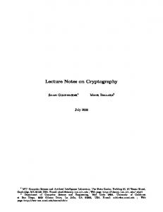
– Functionality assertions correspond to unary key dependencies in databases. Specifically (funct P ) corresponds to stating that the first component of the binary relation P is a key for P , while (funct P − ) states the same for the second component of P . – Identification assertions correspond to more complex forms of key dependencies. To illustrate this correspondence, consider a concept A and a set of attributes U1 , . . . , Un , where each Ui is functional and has A as domain (i.e., the TBox contains the functionality assertion (funct Ui ) and the inclusion assertion δ(Ui ) v A). Together, A and “its attributes” can be considered as representing a single relation RA of arity n + 1 constituted by one column for the object A and one column for each of the Ui attributes. Then, an identification assertion (id A Ui1 , . . . , Uik ), involving a subset Ui1 , . . . , Uik of the attributes of A, resembles a key dependency on RA , where the key is given by the specified subset of attributes. Indeed, due to the identification assertion, a given sequence v1 , . . . , vk of values for Ui1 , . . . , Uik determines a unique instance a of A, and since all attributes are functional and have A as domain, their value is uniquely determined by a, and hence by v1 , . . . , vk . For further intuitions about the meaning of the various kinds of TBox assertions we refer also to Section 3, where the relationship with conceptual models (specifically, UML class diagrams) is discussed in detail. Example 2.3. We conclude this section with an example in which we present a DLLiteA,id ontology modeling the annual national football7 championships in Europe, where the championship for a specific nation is called league (e.g., the Spanish Liga). A 7

Football is called “soccer” in the United States.

I NCLUSION ASSERTIONS League v ∃OF ∃OF v League ∃OF− v Nation Round v ∃BELONGS-TO ∃BELONGS-TO v Round ∃BELONGS-TO− v League Match v ∃PLAYED-IN ∃PLAYED-IN v Match ∃PLAYED-IN− v Round Match v ∃HOME ∃HOME v Match ∃HOME− v Team Match v ∃HOST ∃HOST v Match ∃HOST− v Team F UNCTIONALITY ASSERTIONS (funct OF) (funct HOME) (funct BELONGS-TO) (funct HOST) (funct PLAYED-IN) I DENTIFICATION ASSERTIONS 1. (id League OF, year) 6. (id 2. (id Round BELONGS-TO, code) 7. (id 3. (id Match PLAYED-IN, code) 8. (id 4. (id Match HOME, PLAYED-IN) 9. (id 5. (id Match HOST, PLAYED-IN) 10. (id

PlayedMatch ScheduledMatch PlayedMatch Match League Match Round PlayedMatch PlayedMatch PlayedMatch ρ(date) ρ(homeGoals) ρ(hostGoals) ρ(code) ρ(year)

v Match v Match v ¬ScheduledMatch v ¬Round v δ(year) v δ(code) v δ(code) v δ(date) v δ(homeGoals) v δ(hostGoals) v xsd:date v xsd:nonNegativeInteger v xsd:nonNegativeInteger v xsd:string v xsd:positiveInteger

(funct year) (funct code) (funct date)

(funct homeGoals) (funct hostGoals)

PlayedMatch date, HOST) PlayedMatch date, HOME) League year, BELONGS-TO− ◦ PLAYED-IN− ◦ HOME) League year, BELONGS-TO− ◦ PLAYED-IN− ◦ HOST) Match HOME, HOST, PLAYED-IN ◦ BELONGS-TO ◦ year)

Fig. 3. The DL-LiteA,id TBox Tfbc for the football championship example. league is structured in terms of a set of rounds. Every round contains a set of matches, each one characterized by one home team and one host team. We distinguish between scheduled matches, i.e., matches that have still to be played, and played matches. Obviously, a match falls in exactly one of these two categories. In Figure 2, we show a schematic representation of (a portion of) the intensional part of the ontology for the football championship domain. In this figure, the black arrow represents a partition of one concept into a set of sub-concepts. We have not represented explicitly in the figure the pairwise disjointness of the concepts Team, Match, Round, League, and Nation, which intuitively holds in the modeled domain. In Figure 3, a DL-LiteA,id TBox Tfbc is shown that captures (most of) the above aspects. In our examples, we use the CapitalizedItalics font to denote atomic concepts, the ALL-CAPITALSITALICS font to denote atomic roles, the typewriter font to denote value-domains, and the boldface font to denote atomic attributes. Regarding the pairwise disjointness of the various concepts, we have represented by means of negative inclusion assertions only the disjointness between PlayedMatch and ScheduledMatch and the one between Match and Round. By virtue of the characteristics of DL-LiteA,id , we can explicitly consider also attributes of concepts and the fact that they are used for identification. In particular, we assume that when a scheduled match takes place, it is played in a specific date, and that for every match that has been played, the number of goals scored by the home team and by the host team are given. Note that different matches scheduled for the same round can be played in different dates. Also, we want to distinguish football

C ONCEPT AND ROLE MEMBERSHIP ASSERTIONS League(it2009) BELONGS-TO(r7, it2009) Round(r7) BELONGS-TO(r8, it2009) Round(r8) HOME(m7RJ, roma) PlayedMatch(m7RJ) HOME(m8NT, napoli) Match(m8NT) HOME(m8RM, roma) Match(m8RM) Team(napoli) Team(roma) ATTRIBUTE MEMBERSHIP ASSERTIONS code(r7, "7") code(m7RJ, "RJ") code(r8, "8") code(m8NT, "NT") code(m8RM, "RM")

PLAYED-IN(m7RJ, r7) PLAYED-IN(m8NT, r8) PLAYED-IN(m8RM, r8) HOST(m7RJ, juventus) HOST(m8NT, torino) HOST(m8RM, milan) Team(juventus) date(m7RJ, 5/4/09) homeGoals(m7RJ, 3) hostGoals(m7RJ, 1)

Fig. 4. The ABox Afbc for the football championship example. championships on the basis of the nation and the year in which a championship takes place (e.g., the 2009 Italian Liga). We also assume that both matches and rounds have codes. The identification assertions model the following aspects: 1. 2. 3. 4. 5. 6. 7. 8. 9. 10.

No nation has two leagues in the same year. Within a league, the code associated to a round is unique. Every match is identified by its code within its round. A team is the home team of at most one match per round. As above for the host team. No home team participates in different played matches in the same date. As above for the host team. No home team plays in different leagues in the same year. As above for the host team. No pair (home team, host team) plays different matches in the same year.

Note that the DL-LiteA,id TBox in Figure 3 captures the ontology in Figure 2, except for the fact that the concept Match covers the concepts ScheduledMatch and PlayedMatch. In order to express such a condition, we would need to use disjunction in the right-hand-side of inclusion assertions, i.e., Match v ScheduledMatch t PlayedMatch where t would be interpreted as set union. As we will see in Section 6, we have to renounce to the expressive power required to capture covering constraints (i.e., disjunction), if we want to preserve nice computational properties for reasoning over DLLiteA,id ontologies. An ABox, Afbc , associated to the TBox in Figure 3 is shown in Figure 4, where we have used the slanted font for constants in ΓO and the typeface font for constants in ΓV . For convenience of reading, we have chosen in the example names of the constants that indicate the properties of the objects that the constants represent.

We observe that the ontology Ofbc = hTfbc , Afbc i is satisfiable. Indeed, the interpretation I = (∆I , ·I ) shown in Figure 5 is a model of the ABox Afbc , where we have assumed that for each value constant c ∈ ΓV , the corresponding value val (c) is equal to c itself, hence cI = val (c) = c. Moreover, it is easy to see that every interpretation I has to satisfy the conditions shown in Figure 5 in order to be a model of Afbc . Furthermore, the following are necessary conditions for I to be also a model of the TBox Tfbc , and hence of Ofbc : it2009I ∈ (∃OF)I it2009I ∈ (δ(year))I m7RJI ∈ MatchI torinoI ∈ TeamI milanI ∈ TeamI

to satisfy to satisfy to satisfy to satisfy to satisfy

League v ∃OF, League v δ(year), PlayedMatch v Match, ∃HOST− v Team, ∃HOST− v Team.

Notice that, in order for an interpretation I to satisfy the condition specified in the first row above, there must be an object o ∈ ∆IO such that (it2009I , o) ∈ OFI . According to the inclusion assertion ∃OF− v Nation, such an object o must also belong to NationI (indeed, in our ontology, every league is of one nation). Similarly, the second row above derives from the property that every league must have a year. We note that, besides satisfying the conditions discussed above, an interpretation I 0 may also add other elements to the interpretation of concepts, attributes, or roles specified by I. For instance, the interpretation I 0 that adds to I the object italyI ∈ NationI is still a model of the ontology Ofbc . Note, finally, that there exists no model of Ofbc such that m7RJ is interpreted as an instance of ScheduledMatch, since m7RJ has to be interpreted as an instance of PlayedMatch, and according to the inclusion assertion PlayedMatch v ¬ScheduledMatch, the sets of played matches and of scheduled matches are disjoint.

(it2009I ) ∈ LeagueI (r7I ) ∈ RoundI (r8I ) ∈ RoundI (m7RJI ) ∈ PlayedMatchI (m8NTI ) ∈ MatchI (m8RMI ) ∈ MatchI (romaI ) ∈ TeamI (r7I , "7") ∈ codeI (r8I , "8") ∈ codeI

(r7 , it2009 ) ∈ BELONGS-TO (r8I , it2009I ) ∈ BELONGS-TOI (m7RJI , romaI ) ∈ HOMEI (m8NTI , napoliI ) ∈ HOMEI (m8RMI , romaI ) ∈ HOMEI (napoliI ) ∈ TeamI

(m7RJI , r7I ) ∈ PLAYED-INI (m8NTI , r8I ) ∈ PLAYED-INI (m8RMI , r8I ) ∈ PLAYED-INI (m7RJI , juventusI ) ∈ HOSTI (m8NTI , torinoI ) ∈ HOSTI (m8RMI , milanI ) ∈ HOSTI (juventusI ) ∈ TeamI

(m7RJI , "RJ") ∈ codeI (m8NTI , "NT") ∈ codeI (m8RMI , "RM") ∈ codeI

(m7RJI , 5/4/09) ∈ dateI (m7RJI , 3) ∈ homeGoalsI (m7RJI , 1) ∈ hostGoalsI

I

I

I

Fig. 5. A model of the ABox Afbc for the football championship example.

The above example clearly shows the difference between a database and an ontology. From a database point of view the ontology Ofbc discussed in the example might seem incorrect: for example, while the TBox Tfbc sanctions that every league has a year, there is no explicit year for it2009 in the ABox Afbc . However, the ontology is not incorrect: the axiom stating that every league has a year simply specifies that in every model of Ofbc there will be a year for it2009, even if such a year is not known.

2.3

DL-LiteA,id vs. OWL 2 QL

Having now completed the definition of the syntax and semantics of DL-LiteA,id , we would like to point out that DL-LiteA,id is at the basis of OWL 2 QL, one of the three profiles of OWL 2 that are currently being standardized by the World-Wide-Web Consortium (W3C). The OWL 2 profiles8 are fragments of the full OWL 2 language that have been designed and standardized for specific application requirements. According to (the current version of) the official W3C profiles document, “OWL 2 QL includes most of the main features of conceptual models such as UML class diagrams and ER diagrams. [It] is aimed at applications that use very large volumes of instance data, and where query answering is the most important reasoning task. In OWL 2 QL, conjunctive query answering can be implemented using conventional relational database systems.” We will substantiate all these claims in the next sections. Here, we briefly point out the most important differences between DL-LiteA,id and OWL 2 QL (apart from differences in terminology and syntax, which we do not mention): (1) The main difference is certainly the fact that OWL 2 QL does not adopt the unique name assumption, while such assumption holds for DL-LiteA,id (and the whole DLLite family, in fact). The reason for this semantic mismatch is on the one hand that OWL 2, as most DLs, does not adopt the UNA, and since the profiles are intended to be syntactic fragments of the full OWL 2 language, it was not desirable for a profile to change a basic semantic assumption. On the other hand, the UNA is at the basis of data management in databases, and moreover, by dropping it, DL-LiteA,id would lose its nice computational properties (cf. Theorem 6.6). (2) OWL 2 QL does not allow for expressing functionality of roles or attributes, or identification assertions, while such constructs are present in DL-LiteA,id . This aspect is related to Item (1), and motivated by the fact that the OWL 2 QL profile is intended to have the same nice computational properties as DL-LiteA,id . In order to preserve such properties even in the absence of the UNA, the proof of Theorem 6.6 tells us that we need to avoid the use of functionality (and of identification assertions, since these can be used to simulate functionality). Indeed, as testified also by the complexity results in [4], in the absence of these constructs, the UNA has no impact on complexity of reasoning, and hence OWL 2 QL exhibits the same computational properties as DL-LiteA,id . 8

http://www.w3.org/TR/owl2-profiles/

(3) OWL 2 QL includes the possibility to assert additional role properties, such as disjointness, reflexivity, irreflexivity, symmetry, and asymmetry, that are not explicitly present in DL-LiteA,id . It is immediate to see that disjointness between roles Q1 and Q2 can be expressed by means of Q1 v ¬Q2 , and that reflexivity of a role P can be expressed by means of P v P − . Moreover, as shown in [4], also the addition of irreflexivity, symmetry, and asymmetry does not affect the computational complexity of inference (including query answering, see Section 2.4), and such constructs could be incorporated in the reasoning algorithms for DL-LiteA,id with only minor changes. (4) OWL 2 QL inherits its specific datatypes (corresponding to the value domains of DL-LiteA,id ) from OWL 2, while DL-LiteA,id does not provide any details about datatypes. However, OWL 2 QL imposes restrictions on the allowed datatypes that ensure that no datatype has an unbounded domain, which is sufficient to guarantee that datatypes will not interfere unexpectedly in reasoning. We remark that, due to the correspondence between OWL 2 QL and DL-LiteA,id , all the results and techniques presented in the next sections have a direct impact on OWL 2, i.e., on a standard language for the Semantic Web, that builds on a large user base. Hence, such results are of immediate practical relevance. 2.4

Queries over DL-LiteA,id Ontologies

We are interested in queries over ontologies expressed in DL-LiteA,id . Similarly to the case of relational databases, the basic query class that we consider is the class of unions of conjunctive queries, which is a subclass of the class of First-Order Logic queries. Syntax of Queries. A First-Order Logic (FOL) query q over a DL-LiteA,id ontology O (resp., TBox T ) is a, possibly open, FOL formula ϕ(x) whose predicate symbols are atomic concepts, value-domains, roles, or attributes of O (resp., T ). The free variables of ϕ(x) are those appearing in x, which is a tuple of (pairwise distinct) variables. In other words, the atoms of ϕ(x) have the form A(x), D(x), P (x, y), U (x, y), or x = y, where: – A, F , P , and U are respectively an atomic concept, a value-domain, an atomic role, and an atomic attribute in O, – x, y are either variables in x or constants in Γ . The arity of q is the arity of x. A query of arity 0 is called a boolean query. When we want to make the arity of a query q explicit, we denote the query as q(x). A conjunctive query (CQ) q(x) over a DL-LiteA,id ontology is a FOL query of the form ∃y. conj (x, y), where y is a tuple of pairwise distinct variables not occurring among the free variables x, and where conj (x, y) is a conjunction of atoms. The variables x are also called distinguished and the (existentially quantified) variables y are called non-distinguished. We will also make use of conjunctive queries with inequalities, which are CQs in which also atoms of the form x 6= y (called inequalities) may appear.

A union of conjunctive queries (UCQ) is a FOL query that is the disjunction of a set of CQs of the same arity, i.e., it is a FOL formula of the form: ∃y 1 . conj 1 (x, y 1 ) ∨ · · · ∨ ∃y n . conj n (x, y n ). UCQs with inequalities are obvious extensions of UCQs. Finally, a positive FOL query is a FOL query ϕ(x) where the formula ϕ is built using only conjunction, disjunction, and existential quantification (i.e., it contains neither negation nor universal quantification). Datalog Notation for CQs and UCQs. In the following, it will sometimes be convenient to consider a UCQ as a set of CQs, rather than as a disjunction of UCQs. We will also use the Datalog notation for CQs and UCQs. In this notation, a CQ is written as q(x) ← conj 0 (x, y) and a UCQ is written as a set of CQs q(x) ← conj 01 (x, y 1 ) .. . q(x) ← conj 0n (x, y n ) where conj 0 (x, y) and each conj 0i (x, y i ) in a CQ are considered simply as sets of atoms (written in list notation, using a ‘,’ as a separator). In this case, we say that q(x) is the head of the query, and that conj 0 (x, y) and each conj 0i (x, y i ) is the body of the corresponding CQ. Semantics of Queries. Given an interpretation I = (∆I , ·I ), the FOL query q = ϕ(x) is interpreted in I as the set q I of tuples o ∈ ∆I × · · · × ∆I such that the formula ϕ evaluates to true in I under the assignment that assigns each object in o to the corresponding variable in x [1]. We call q I the answer to q over I. Notice that the answer to a boolean query is either the empty tuple, “()”, considered as true, or the empty set, considered as false. We remark that a relational database (over the atomic concepts, roles, and attributes) corresponds to a finite interpretation. Hence the notion of answer to a query introduced here is the standard notion of answer to a query evaluated over a relational database. In the case where the query is a CQ, the above definition of answer can be rephrased in terms of homomorphisms. In general, a homomorphisms between two interpretations (i.e., First-Order structures) is defined as follows. Definition 2.4. Given two interpretations I = (∆I , ·I ) and J = (∆J , ·J ) over the same set P of predicate symbols, a homomorphism µ from I to J is a mapping µ : ∆I → ∆J such that, for each predicate P ∈ P of arity n and each tuple (o1 , . . . , on ) ∈ (∆I )n , if (o1 , . . . , on ) ∈ P I , then (µ(o1 ), . . . , µ(on )) ∈ P J .

Notice that, in the case of interpretations of a DL-LiteA,id ontology, the set of predicate symbols in the above definition would be the set of atomic concepts, value domains, roles, and attributes of the ontology. We can now extend the definition to consider also homomorphisms from CQs to interpretations. Definition 2.5. Given a CQ q(x) = ∃y. conj (x, y) over interpretation I = (∆I , ·I ), and a tuple o = (o1 , . . . , on ) of objects of ∆I of the same arity as x = (x1 , . . . , xn ), a homomorphism from q(o) to I is a mapping µ from the variables and constants in q(x) to ∆I such that: – µ(c) = cI , for each constant c in conj (x, y), – µ(xi ) = oi , for i ∈ {1, . . . , n}, and – (µ(t1 ), . . . , µ(tn )) ∈ P I , for each atom P (t1 , . . . , tn ) that appears in conj (x, y). The following result established in [33] provides a fundamental characterization of answers to CQs in terms of homomorphism. Theorem 2.6 ([33]). Given a CQ q(x) = ∃y. conj (x, y) over an interpretation I = (∆I , ·I ), and a tuple o = (o1 , . . . , on ) of objects of ∆I of the same arity as x = (x1 , . . . , xn ), we have that o ∈ q I if and only if there is a homomorphism from q(o) to I. In fact, the notion of homomorphism is crucial in the context of the study of CQs, and most inference tasks involving CQs (including query containment [59], and tasks related to view-based query processing [47]) can be rephrased in terms of homomorphism [1]. Example 2.7. Consider again the ontology Ofbc = hTfbc , Afbc i introduced in Example 2.3, and the following query asking for all matches: q1 (x) ← Match(x). If I is the interpretation shown in Figure 5, we have that:

q1I = {(m8NTI ), (m8RMI )}.

Notice that I is a model of Afbc , but not of Tfbc . Let instead I 0 be the interpretation analogous to I, but extended in such a way that it becomes also a model of Tfbc , and hence of Ofbc , as shown in Example 2.3. Then we have that: 0

q1I = {(m8NTI ), (m8RMI ), (m7RJI )}. Suppose now that we ask for teams, together with the code of the match in which they have played as home team: q2 (t, c) ← Team(t), HOME(m, t), Match(m), code(m, c). Then we have that q2I = {(napoliI , "NT"), (romaI , "RM")}, 0 q2I = {(romaI , "RJ"), (napoliI , "NT"), (romaI , "RM")}.

Certain Answers. The notion of answer to a query introduced above is not sufficient to capture the situation where a query is posed over an ontology, since in general an ontology will have many models, and we cannot single out a unique interpretation (or database) over which to answer the query. Instead, the ontology determines a set of interpretations, i.e., the set of its models, which intuitively can be considered as the set of databases that are “compatible” with the information specified in the ontology. Given a query, we are interested in those answers to this query that depend only on the information in the ontology, i.e., that are obtained by evaluating the query over a database compatible with the ontology, but independently of which is the actually chosen database. In other words, we are interested in those answers to the query that are obtained for all possible databases (including infinite ones) that are models of the ontology. This corresponds to the fact that the ontology conveys only incomplete information about the domain of interest, and we want to guarantee that the answers to a query that we obtain are certain, independently of how we complete this incomplete information. This leads us to the following definition of certain answers to a query over an ontology. Definition 2.8. Let O be a DL-LiteA,id ontology and q a UCQ over O. A tuple c of constants appearing in O is a certain answer to q over O, written c ∈ cert(q, O), if for every model I of O, we have that cI ∈ q I . Answering a query q posed to an ontology O means exactly to compute the set of certain answers to q over O. Example 2.9. Consider again the ontology introduced in Example 2.3, and queries q1 and q2 introduced in Example 2.7. One can easily verify that cert(q1 , O) = {(m8NTI ), (m8RMI ), (m7RJI )}, cert(q2 , O) = {(romaI , "RJ"), (napoliI , "NT"), (romaI , "RM")}. Notice that, in the case where O is an unsatisfiable ontology, the set of certain answers to a (U)CQ q is the finite set of all possible tuples of constants whose arity is the one of q. We denote such a set by AllTup(q, O). 2.5

Reasoning Services

In studying DL-LiteA,id , we are interested in several reasoning services, including the traditional DL reasoning services. Specifically, we consider the following problems for DL-LiteA,id ontologies: – Ontology satisfiability, i.e., given an ontology O, verify whether O admits at least one model. – Concept and role satisfiability, i.e., given a TBox T and a concept C (resp., a role R), verify whether T admits a model I such that C I 6= ∅ (resp., RI 6= ∅). – We say that an ontology O (resp., a TBox T ) logically implies an assertion α, denoted O |= α (resp., T |= α, if every model of O (resp., T ) satisfies α. The problem of logical implication of assertions consists of the following sub-problems:

• instance checking, i.e., given an ontology O, a concept C and a constant a (resp., a role R and a pair of constants a1 and a2 ), verify whether O |= C(a) (resp., O |= R(a1 , a2 )); • subsumption of concepts or roles, i.e., given a TBox T and two general concepts C1 and C2 (resp., two general roles R1 and R2 ), verify whether T |= C1 v C2 (resp., T |= R1 v R2 ); • checking functionality, i.e., given a TBox T and a basic role Q, verify whether T |= (funct Q). • checking an identification constratins, i.e., given a TBox T and an identification constraint (id C π1 , . . . , πn ), verify whether T |= (id C π1 , . . . , πn ). In addition we are interested in: – Query answering, i.e., given an ontology O and a query q (either a CQ or a UCQ) over O, compute the set cert(q, O). The following decision problem, called recognition problem, is associated to the query answering problem: given an ontology O, a query q (either a CQ or a UCQ), and a tuple of constants a of O, check whether a ∈ cert(q, O). When we talk about the computational complexity of query answering, in fact we implicitly refer to the associated recognition problem. In analyzing the computational complexity of a reasoning problem over a DL ontology, we distinguish between data complexity and combined complexity [91]: data complexity is the complexity measured with respect to the size of the ABox only, while combined complexity is the complexity measured with respect to the size of all inputs to the problem, i.e., the TBox, the ABox, and the query. The data complexity measure is of interest in all those cases where the size of the intensional level of the ontology (i.e., the TBox) is negligible w.r.t. the size of the data (i.e., the ABox), as in ontology-based data access (cf. Section 1.3). 2.6

The Notion of FOL-rewritability

We now introduce the notion of FOL-rewritability for both satisfiability and query answering, which will be used in the sequel. First, given an ABox A (of the kind considered above), we denote by DB (A) = h∆DB(A) , ·DB(A) i the interpretation defined as follows:

– ∆DB(A) is the non-empty set consisting of the union of the set of all object constants occurring in A and the set {val (c) | c is a value constant that occurs in A}, – aDB(A) = a, for each object constant a, – ADB(A) = {a | A(a) ∈ A}, for each atomic concept A, – P DB(A) = {(a1 , a2 ) | P (a1 , a2 ) ∈ A}, for each atomic role P , and – U DB(A) = {(a, val (c)) | U (a, c) ∈ A}, for each atomic attribute U .

Observe that the interpretation DB (A) is a minimal model of the ABox A. Intuitively, FOL-rewritability of satisfiability (resp., query answering) captures the property that we can reduce satisfiability checking (resp., query answering) to evaluating a FOL query over the ABox A considered as a relational database, i.e., over DB (A). The definitions follow.

Definition 2.10. Satisfiability in a DL L is FOL-rewritable, if for every TBox T expressed in L, there exists a boolean FOL query q, over the alphabet of T , such that for every non-empty ABox A, the ontology hT , Ai is satisfiable if and only if q evaluates to false in DB (A). Definition 2.11. Answering UCQs in a DL L is FOL-rewritable, if for every UCQ q and every TBox T expressed over L, there exists a FOL query q1 , over the alphabet of T , such that for every non-empty ABox A and every tuple of constants a occurring in DB(A) A, we have that a ∈ cert(q, hT , Ai) if and only if aDB(A) ∈ q1 . We remark that FOL-rewritability of a reasoning problem that involves the ABox of an ontology (such as satisfiability or query answering) is tightly related to the data complexity of the problem. Indeed, since the FOL query considered in the above definitions depends only on the TBox (and the query), but not on the ABox, and since the evaluation of a First-Order Logic query (i.e., an SQL query without aggregation) over an ABox is in AC0 in data complexity [1], FOL-rewritability of a problem has as an immediate consequence that the problem is in AC0 in data complexity. Hence, one way of showing that for a certain DL L a problem is not FOL-rewritable, is to show that the data complexity of the problem for the DL L is above AC0 , e.g., L OG S PACE-hard, NL OG S PACE-hard, PT IME-hard, or even coNP-hard. We will provide some results of this form in Section 6 (see also [4]).

3

UML Class Diagrams as an Ontology Language

In this section, we discuss how UML class diagrams can be considered as an ontology language, and we show how such diagrams can be captured in DL-LiteA,id . Since we concentrate on class diagrams from the conceptual perspective, we do not deal with those features that are more relevant for the software engineering perspective, such as operations (methods) associated to classes, or public, protected, and private qualifiers for methods and attributes. Also, for sake of brevity and to smooth the presentation we make some simplifying assumptions that could all be lifted without changing the results presented here (we refer to [11] for further details). In particular, we will not deal explicitly with associations of arity greater than 2, and we will only deal with the following multiplicities: – unconstrained, i.e., 0..∗, – functional participation, i.e., 0..1, – mandatory participation, i.e., 1..∗, and – one-to-one correspondence, i.e., 1..1. These multiplicities are particularly important since they convey meaningful semantic aspects in modeling, and thus are the most commonly used ones. Our goal is twofold. On the one hand, we aim at showing how class diagrams can be expressed in DLs. On the other hand, we aim at understanding which is the complexity of inference over an UML class diagram. We will show that the formalization in DLs helps us in deriving complexity results both for reasoning and for query answering over an UML class diagram.

3.1

Classes and Attributes

A class in a UML class diagram denotes a sets of objects with common features. The specification of a class contains its name and its attributes, each denoted by a name (possibly followed by the multiplicity, between square brackets) and with an associated type, which indicates the domain of the attribute values. A UML class is represented by a DL concept. This follows naturally from the fact that both UML classes and DL concepts denote sets of objects. A UML attribute a of type T for a class C associates to each instance of C, zero, one, or more instances of type T . An optional multiplicity [i..j] for a specifies that a associates to each instance of C, at least i and most j instances of T . When the multiplicity for an attribute is missing, [1..1] is assumed, i.e., the attribute is mandatory and single-valued. To formalize attributes, we have to think of an attribute a of type T for a class C as a binary relation between instances of C and instances of T . We capture such a binary relation by means of a DL attribute aC . To specify the type of the attribute we use the DL assertions δ(aC ) v C, ρ(aC ) v T.

Such assertions specify precisely that, for each instance (c, v) of the attribute aC , the object c is an instance of C, and the value v is an instance of T . Note that the attribute name a is not necessarily unique in the whole diagram, and hence two different classes, say C and C 0 could both have attribute a, possibly of different types. This situation is correctly captured in the DL formalization, where the attribute is contextualized to each class with a distinguished DL attribute, i.e., aC and aC 0 . To specify that the attribute is mandatory (i.e., multiplicity [1..∗]), we add the assertion C v δ(aC ), which specifies that each instance of C participates necessarily at least once to the DL attribute aC . To specify that the attribute is single-valued (i.e., multiplicity [0..1]), we add the functionality assertion (funct aC ). Finally, if the attribute is both mandatory and single-valued (i.e., multiplicity [1..1]), we use both assertions together, i.e., C v δ(aC ), 3.2

(funct aC ).

Associations

An association in UML is a relation between the instances of two (or more) classes. An association often has a related association class that describes properties of the association, such as attributes, operations, etc. A binary association A between the instances of two classes C1 and C2 is graphically rendered as in Figure 6(a), where the multiplicity m` ..mu specifies that each instance of class C1 can participate at least m` times and at most mu times to association A. The multiplicity n` ..nu has an analogous meaning for class C2 .

C1 C1

n! ..nu

A

m! ..mu

n! ..nu RA,1

C2

m! ..mu RA,2

C2

A

(a) Without association class.

(b) With association class.

Fig. 6. Associations in UML.

An association A between classes C1 and C2 is formalized in DL by means of a role A on which we enforce the assertions ∃A v C1 ,

∃A− v C2 .

To express the multiplicity m` ..mu on the participation of instances of C2 for each given instance of C1 , we use the assertion C1 v ∃A, if m` = 1, and (funct A), if mu = 1. We can use similar assertions for the multiplicity n` ..nu on the participation of instances of C1 for each given instance of C2 , i.e., C2 v ∃A− , if n` = 1, and (funct A− ), if nu = 1. Next we focus on associations with a related association class, as shown in Figure 6(b), where the class A is the association class related to the association, and RA,1 and RA,2 , if present, are the role names of C1 and C2 respectively, i.e., they specify the role that each class plays within the association A. We formalize in DL an association A with an association class, by reifying it into a DL concept A and introducing two DL roles RA,1 , RA,2 , one for each role of A, which intuitively connect an object representing an instance of the association respectively to the instances of C1 and C2 that participate to the association9 . Then, we enforce that each instance of A participates exactly once both to RA,1 and to RA,2 , by means of the assertions A v ∃RA,1 ,

(funct RA,1 ),

A v ∃RA,2 ,

(funct RA,2 ).

To represent that the association A is between classes C1 and C2 , we use the assertions ∃RA,1 v A,

− ∃RA,1 v C1 ,

∃RA,2 v A,

− ∃RA,2 v C2 .

Finally, we use the assertion (id A RA,1 , RA,2 ) to specify that each instance of the concept A represents a distinct tuple in C1 × C2 .10 We can easily represent in DL multiplicities on an association with association class, by imposing suitable assertions on the inverses of the DL roles modeling the roles of 9 10

If the roles of the association are not available, we may use an arbitrary DL role name. Notice that such an approach can immediately be used to represent an association of any arity: it suffices to repeat the above for every component.

C {disjoint, complete}

C1

Cn

C2

Fig. 7. A class hierarchy in UML. the association. For example, to say that there is a one-to-one participation of instances of C1 in the association (with related association class) A, we assert − C1 v ∃RA,1 ,

3.3

− (funct RA,1 ).

Generalizations and Class Hierarchies

In UML, one can use generalization between a parent class and a child class to specify that each instance of the child class is also an instance of the parent class. Hence, the instances of the child class inherit the properties of the parent class, but typically they satisfy additional properties that in general do not hold for the parent class. Generalization is naturally supported in DLs. If a UML class C2 generalizes a class C1 , we can express this by the DL assertion C1 v C2 . Inheritance between DL concepts works exactly as inheritance between UML classes. This is an obvious consequence of the semantics of v, which is based on the subset relation. As a consequence, in the formalization, each attribute of C2 and each association involving C2 is correctly inherited by C1 . Observe that the formalization in DL also captures directly multiple inheritance between classes. In UML, one can group several generalizations into a class hierarchy, as shown in Figure 7. Such a hierarchy is captured in DL by a set of inclusion assertions, one between each child class and the parent class, i.e., Ci v C,

for each i ∈ {1, . . . , n}.

Often, when defining generalizations between classes, we need to add additional assertions among the involved classes. For example, for the class hierarchy in Figure 7, an assertion may express that C1 , . . . , Cn are mutually disjoint. In DL, such a relationship can be expressed by the assertions Ci v ¬Cj ,

for each i, j ∈ {1, . . . , n} with i 6= j.

Moreover, we may want to express that a generalization hierarchy is complete, i.e., that the subclasses C1 , . . . , Cn are a covering of the superclass C. We can represent such a situation in DL by including the additional assertion C v C1 t · · · t Cn .

C21

RA2,1

RA2,2

C22

A2 C11

RA1,1

RA1,2

C12

A1

Fig. 8. A generalization between association classes in UML.

Such an assertion models a form of disjunctive information: each instance of C is either an instance of C1 , or an instance of C2 , . . . or an instance of Cn . Notice, however, that the use of concept disjunction, and hence of the inclusion assertion above, is not allowed in DL-LiteA,id . 3.4

Subset Assertions between Associations

Similarly to generalization between classes, UML allows one to state subset assertions between associations. A subset assertion between two associations A1 and A2 can be modeled in DL by means of the role inclusion assertion A1 v A2 , involving the two DL roles A1 and A2 representing the associations. Notice that this is allowed in DL-LiteA,id only if none of the maximum multiplicities of the two classes participating to A2 is equal to 1. With respect to a generalization between two association classes A1 and A2 , we note that to correctly capture the corresponding subset assertion between the associations represented by the association classes, we would need to introduce not only inclusion assertions between the concepts representing the association classes, but also between the DL roles representing corresponding roles of A1 and A2 . Consider, for example, the generalization between association classes depicted in Figure 8. We can correctly capture the two associations with association classes A1 and A2 by the following DL assertions: A1 v ∃RA1,1 , (funct RA1,1 ), A1 v ∃RA1,2 , (funct RA1,2 ), − ∃RA1,1 v A1 , ∃RA1,1 v C11 , − ∃RA1,2 v A1 , ∃RA1,2 v C12 , (id A1 RA1,1 , RA1,2 ),

A2 v ∃RA2,1 , (funct RA2,1 ), A2 v ∃RA2,2 , (funct RA2,2 ), − ∃RA2,1 v A2 , ∃RA2,1 v C21 , − ∃RA2,2 v A2 , ∃RA2,2 v C22 , (id A2 RA2,1 , RA2,2 ).

Finally, to capture the generalization, we could use the following inclusion assertions A1 v A2 ,

RA1,1 v RA2,1 ,

RA1,2 v RA2,2 .

However, since RA2,1 and RA2,2 are functional roles (and are also used in an identification assertion), we actually cannot specialize them, if we want to stay in DL-LiteA,id . Hence, generalization of associations with association classes in general cannot be formalized in DL-LiteA,id . Finally, we observe that a formalization in DL-LiteA,id of generalization between association classes is possible if the sub-association does not specify new classes for the domain and range of the association with respect to the super-association. In the example of Figure 8 this would mean that C11 coincides with C21 and C12 coincides with C22 . In this case, the sub-association A1 is represented by simply using the same DL roles as for A2 to denote its components. Hence, it is not necessary to introduce an inclusion assertion between functional DL roles to correctly capture the generalization between association classes.

3.5

Reasoning and Query Answering over UML Class Diagrams

The fact that UML class diagrams can be captured by DLs enables the possibility of performing sound and complete reasoning to do formal verification at design time and query answering at runtime, as will be illustrated in the next sections. Hence, one can exploit such ability to get support during the design phase of an ontology-based data access system, and to take the information in the UML class diagram fully into account during query answering. It was shown in [11] that, unfortunately, reasoning (in particular checking the consistency of the diagram, a task to which other typical reasoning tasks of interest reduce) is E XP T IME-hard. What this result tells us is that, if the TBox is expressed in UML, then the support at design time for an ontology-based data access system may be difficult to obtain if the schema has a reasonable size. Turning to query answering, the situation is even worse. The results in Section 6 imply that answering conjunctive queries in the presence of a UML class diagram formed by a single generalization with covering assertion is coNP-hard in the size of the instances of classes and associations. Hence, query answering over even moderately large data sets is again infeasible in practice. It is not difficult to see that this implies that, in an ontology-based data access system where the TBox is expressed as a UML diagram, answering conjunctive queries is coNP-hard with respect to the size of the data in the accessed source. Actually, as we will see in Section 6, one culprit of such a high complexity is the ability of expressing covering assertions, which induces reasoning by cases. A further cause of high complexity is the unrestricted interaction between multiplicities (actually, functionality) and subset constraints between associations [23,4]. Once we disallow covering and suitably restrict the simultaneous use of subset constraints between associations and multiplicities, not only the sources of exponential complexity disappear, but actually query answering becomes reducible to standard SQL evaluation over a relational database, as will be demonstrated in the following.

4

Reasoning over Ontologies

In this section, we study traditional DL reasoning services for ontologies. In particular, we consider the reasoning services described in Section 2.5, and we show that all such reasoning services are in PT IME w.r.t. combined complexity, and that instance checking and satisfiability (which make use of the ABox) are FOL-rewritable, and hence in AC0 with respect to data complexity. We concentrate in this section on DL-LiteA ontologies and address the addition of identification assertions in Section 5.6, after having discussed in Section 5 query answering based on reformulation. We deal first with ontology satisfiability, and then we tackle concept and role satisfiability, and logical implication. In fact, we will show that the latter reasoning services can be basically reduced to ontology satisfiability. Finally, we provide the complexity results mentioned above. In the following, to ease the presentation, we make several simplifying assumptions that however do not affect the generality of the presented results: 1. Since the distinction between objects and values does not have an impact on the ontology reasoning services, we will deal only with ontologies that contain object constants, concepts, and roles only, and do not consider value constants, value domains, and attributes. Hence, we also rule out concepts of the form δ(U ) and δF (U ). With respect to the semantics, since we don’t have to deal with values, we consider only interpretations I where the domain of values ∆IV is empty, hence the interpretation domain ∆I coincides with the domain of objects ∆IO . 2. We will assume that the ontology does not contain qualified existential restrictions, i.e., concepts of the form ∃Q.C. Notice that in DL-LiteA,id such concepts may appear only in the right-hand side of inclusion assertions of the form B v ∃Q.C, and only if the role Q and its inverse do not appear in a functionality assertion. We can replace the inclusion assertion B v ∃Q.C by the inclusion assertions B v ∃Pnew − v C ∃Pnew Pnew v Q

where Pnew is a fresh atomic role. It is easy to see that the resulting ontology preserves all reasoning services over the original ontology. By repeated application of the above transformation, once for each occurrence of a concept ∃Q.C in the ontology obtained from the previous application11 , we obtain an ontology that does not contain qualified existential restrictions and that preserves all reasoning services over the original ontology. 3. Since inclusion assertions of the form B v >c do not have an impact on the semantics, we can simply discard them in reasoning. Hence, in the following, we will consider the following simplified grammar for DLLiteA expressions: B C 11

−→ −→

A | ∃Q B | ¬B

Q −→ R −→

P | P− Q | ¬Q

Note that an ontology may contain concepts in which qualified existential restrictions are nested within each other.

Our first goal is to show that ontology satisfiability is FOL-rewritable. To this aim, we resort to two main constructions, namely the canonical interpretation and the closure of the negative inclusions, which we present below. We recall that assertions of the form B1 v B2 or Q1 v Q2 are called positive inclusions (PIs), and assertions of the form B1 v ¬B2 or Q1 v ¬Q2 are called negative inclusions (NIs). Notice that due to the simplified form of the grammar that we are adopting here, these are the only kinds of inclusion assertions that we need to consider. 4.1

Canonical Interpretation

The canonical interpretation of a DL-LiteA ontology is an interpretation constructed according to the notion of chase [1]. In particular, we adapt here the notion of restricted chase adopted by Johnson and Klug in [57]. We start by defining the notion of applicable positive inclusion assertions (PIs), and then we exploit applicable PIs to construct the chase for a DL-LiteA ontology. Finally, with the notion of chase in place, we give the definition of canonical interpretation. In the following, for easiness of exposition, we make use of the following notation for a basic role Q and two constants a1 and a2 : ( P (a1 , a2 ), if Q = P, Q(a1 , a2 ) denotes P (a2 , a1 ), if Q = P − . Definition 4.1. Let S be a set of DL-LiteA membership assertions. Then, a PI α is applicable in S to a membership assertion β ∈ S if – α = A1 v A2 , β = A1 (a), and A2 (a) ∈ / S; – α = A v ∃Q, β = A(a), and there does not exist any constant a0 such that Q(a, a0 ) ∈ S; – α = ∃Q v A, β = Q(a, a0 ), and A(a) ∈ / S; – α = ∃Q1 v ∃Q2 , β = Q1 (a1 , a2 ), and there does not exist any constant a02 such that Q2 (a1 , a02 ) ∈ S; – α = Q1 v Q2 , β = Q1 (a1 , a2 ), and Q2 (a1 , a2 ) ∈ / S. Applicable PIs can be used, i.e., applied, in order to construct the chase of an ontology. Roughly speaking, the chase of a DL-LiteA ontology O = hT , Ai is a (possibly infinite) set of membership assertions, constructed step-by-step starting from the ABox A. At each step of the construction, a PI α ∈ T is applied to a membership assertion β belonging to the current set S of membership assertions. Applying a PI means adding a new suitable membership assertion to S, thus obtaining a new set S 0 in which α is not applicable to β anymore. For example, if α = A1 v A2 is applicable in S to β = A1 (a), the membership assertion to be added to S is A2 (a), i.e., S 0 = S ∪ A2 (a). In some cases (i.e., α = A v ∃Q or α = ∃Q1 v ∃Q2 ), to achieve an analogous aim, the new membership assertion has to make use of a new constant symbol that does not occur in S. Notice that such a construction process strongly depends on the order in which we select both the PI to be applied at each step and the membership assertion to which such

a PI is applied, as well as on which constants we introduce at each step. Therefore, a number of syntactically distinct sets of membership assertions might result from this process. However, it is possible to show that the result is unique up to renaming of constants occurring in each such a set. Since we want our construction process to result in a unique chase of a certain ontology, along the lines of [57], we assume in the following to have a fixed infinite set of constants, whose symbols are ordered in lexicographic way, and we select PIs, membership assertions and constant symbols in lexicographic order. More precisely, given a ontology O = hT , Ai, we denote with ΓA the set of all constant symbols occurring in A. Also, we assume to have an infinite set ΓN of constant symbols not occurring in A, such that the set ΓC = ΓA ∪ ΓN is totally ordered in lexicographic way. Then, our notion of chase is precisely given below. Definition 4.2. Let O = hT , Ai be a DL-LiteA ontology, let Tp be the set of positive inclusion assertions in T , let n be the number of membership assertions in A, and let ΓN be the set of constants defined above. Assume that the membership assertions in A are numbered from 1 to n following their lexicographic order, and consider the following definition of sets Sj of membership assertions: – S0 = A – Sj+1 = Sj ∪ {βnew }, where βnew is a membership assertion numbered with n + j + 1 in Sj+1 and obtained as follows: let β be the first membership assertion in Sj such that there exists a PI α ∈ Tp applicable in Sj to β let α be the lexicographically first PI applicable in Sj to β let anew be the constant of ΓN that follows lexicographically all constants in Sj case α, β of (cr1) α = A1 v A2 and β = A1 (a) then βnew = A2 (a) (cr2) α = A v ∃Q and β = A(a) then βnew = Q(a, anew ) (cr3) α = ∃Q v A and β = Q(a, a0 ) then βnew = A(a) (cr4) α = ∃Q1 v ∃Q2 and β = Q1 (a, a0 ) then βnew = Q2 (a, anew ) (cr5) α = Q1 v Q2 and β = Q1 (a, a0 ) then βnew = Q2 (a, a0 ). Then, we call chase of O, denoted chase(O), the set of membership assertions obtained as the infinite union of all Sj , i.e., chase(O) =

[ j∈N

Sj .

In the above definition, cr1, cr2, cr3, cr4, and cr5 indicate the five rules that are used for constructing the chase, each one corresponding to the application of a PI. Such rules are called chase rules, and we say that a chase rule is applied to a membership assertion β if the corresponding PI is applied to β. Observe also that NIs and functionality assertions in O have no role in constructing chase(O). Indeed chase(O) depends only on the ABox A and the PIs in T . In the following, we will denote with chase i (O) the portion of the chase obtained after i applications of the chase rules, selected according to the ordering established in

Definition 4.2, i.e., chase i (O) =

[ j∈{0,..,i}

Sj .

The following property shows that the notion of chase of an ontology is fair. Proposition 4.3. Let O = hT , Ai be a DL-LiteA ontology, and let α be a PI in T . Then, if there is an i ∈ N such that α is applicable in chase i (O) to a membership assertion β ∈ chase i (O), then there is a j ≥ i such that chase j+1 (O) = chase j (O) ∪ β 0 , where β 0 is the result of applying α to β in chase j (O). Proof. Assume by contradiction that there is no j ≥ i such that chase j+1 (O) = chase j (O) ∪ β 0 . This would mean that either there are infinitely many membership assertions that precede β in the ordering that we choose for membership assertions in chase(O), or that there are infinitely many chase rules applied to some membership assertion that precedes β. However, none of these cases is possible. Indeed, β is assigned with an ordering number m such that exactly m − 1 membership assertions precede β. Furthermore, a PI can be applied at most once to a membership assertion (afterwards, the precondition is not satisfied and the PI is not applicable anymore), and also there exists only a finite number ` of PIs. Therefore, it is possible to apply a chase rule to some membership assertion at most ` times. We can thus conclude that the claim holds. t u With the notion of chase in place we can introduce the notion of canonical interpretation. Definition 4.4. The canonical interpretation can(O) = h∆can(O) , ·can(O) i is the interpretation where: – – – –

∆can(O) = ΓC , acan(O) = a, for each constant a occurring in chase(O), Acan(O) = {a | A(a) ∈ chase(O)}, for each atomic concept A, and P can(O) = {(a1 , a2 ) | P (a1 , a2 ) ∈ chase(O)}, for each atomic role P .

We also define can i (O) = h∆can(O) , ·can i (O) i, where ·can i (O) is analogous to ·can(O) , except that it refers to chase i (O) instead of chase(O). According to the above definition, it is easy to see that can(O) (resp., can i (O)) is unique. Notice also that can 0 (O) is tightly related to the interpretation DB (A). Indeed, while ∆DB(A) ⊆ ∆can(O) , we have that ·DB(A) = ·can 0 (O) . We point out that chase(O) and can(O) (resp., chase i (O)) and can i (O)) are strongly connected. In particular, we note that, whereas chase i+1 (O) is obtained by adding a membership assertion to chase i (O), can i+1 (O) can be seen as obtained from can i (O) by adding either an object to the extension of an atomic concept of O, or a pair of objects to the extension of an atomic role of O (notice that the domain of interpretation is the same in each can i (O), and in particular in can(O)). By virtue of the strong connection discussed above, in the following we will often prove properties of can(O) (resp., can i (O)) by reasoning over the structure of chase(O) (resp., chase i (O)). Now, we are ready to show a notable property that holds for can(O).

Lemma 4.5. Let O = hT , Ai be a DL-LiteA ontology and let Tp be the set of positive inclusion assertions in T . Then, can(O) is a model of hTp , Ai. Proof. Since hTp , Ai does not contain NIs and functionality assertions, to prove the claim we only need to show that can(O) satisfies all membership assertions in A and all PIs in Tp . The fact that can(O) satisfies all membership assertions in A follows from the fact that A ⊆ chase(O). Then, it remains to prove that can(O) |= Tp . Let us proceed by contradiction, considering all possible cases: 1. Assume by contradiction that a PI of the form A1 v A2 ∈ Tp , where A1 and A2 are atomic concepts, is not satisfied by can(O). This means that there exists a constant a ∈ ΓC such that A1 (a) ∈ chase(O) and A2 (a) ∈ / chase(O). However, such a situation would trigger the chase rule cr1, since A1 v A2 would be applicable to A1 (a) in chase(O) and Proposition 4.3 ensures that such a PI would be applied at some step in the construction of the chase, thus causing the insertion of A2 (a) in chase(O). This contradicts the assumption. 2. Assume by contradiction that a PI of the form A v ∃Q ∈ Tp , where A is an atomic concept and Q is a basic role, is not satisfied by can(O). This means that there exists a constant a ∈ ΓC such that A(a) ∈ chase(O) and there does not exist a constant a1 ∈ ΓC such that Q(a, a1 ) ∈ chase(O). However, such a situation would trigger the chase rule cr2, since A v ∃Q would be applicable to A(a) in chase(O) and Proposition 4.3 ensures that such a PI would be applied at some step in the construction of the chase, thus causing the insertion of Q(a, a2 ) in chase(O), where a2 ∈ ΓC follows lexicographically all constants occurring in chase(O) before the execution of cr2. This contradicts the assumption. 3. Assume by contradiction that a PI of the form ∃Q v A ∈ Tp , where Q is a basic role and A is an atomic concept, is not satisfied by can(O). This means that there exists a pair of constants a, a1 ∈ ΓC such that Q(a, a1 ) ∈ chase(O) and A(a) ∈ / chase(O). However, such a situation would trigger the chase rule cr3, since ∃Q v A would be applicable to Q(a, a1 ) in chase(O) and Proposition 4.3 ensures that such a PI would be applied at some step in the construction of the chase, thus causing the insertion of A(a) in chase(O). This contradicts the assumption. 4. Assume by contradiction that a PI of the form ∃Q1 v ∃Q2 ∈ Tp , where Q1 and Q2 are basic roles, is not satisfied by can(O). This means that there exists a pair of constants a, a1 ∈ ΓC such that Q1 (a, a1 ) ∈ chase(O) and there does not exist a constant a2 ∈ ΓC such that Q2 (a, a2 ) ∈ chase(O). However, such a situation would trigger the chase rule cr4 since ∃Q1 v ∃Q2 would be applicable to Q1 (a, a1 ) in chase(O) and Proposition 4.3 ensures that such a PI would be applied at some step in the construction of the chase, thus causing the insertion of Q(a, a3 ) in chase(O), where a3 ∈ ΓC follows lexicographically all constants occurring in chase(O) before the execution of cr4. This contradicts the assumption. 5. Assume by contradiction that a PI of the form Q1 v Q2 ∈ Tp , where Q1 and Q2 are basic roles, is not satisfied by can(O). This means that there exists a pair of constants a, a1 ∈ ΓC such that Q1 (a, a1 ) ∈ chase(O) and Q2 (a, a1 ) ∈ / chase(O). However, such a situation would trigger the chase rule cr5, since Q1 v Q2 would be applicable to Q1 (a, a1 ) in chase(O) and Proposition 4.3 ensures that such a PI

would be applied at some step in the construction of the chase, thus causing the insertion of Q2 (a, a1 ) in chase(O). This contradicts the assumption. t u As a consequence of Lemma 4.5, every DL-LiteA ontology O = hT , Ai with only positive inclusions in the TBox, i.e., such that T = Tp , is always satisfiable, since we can always construct can(O), which is a model for O. Now, one might ask if and how can(O) can be exploited for checking the satisfiability of an ontology with also negative inclusions and functionality assertions. As for functionality assertions, the following lemma shows that, to establish that they are satisfied by can(O), we have to simply verify that the interpretation DB (A) satisfies them (and vice-versa). Lemma 4.6. Let O = hT , Ai be a DL-LiteA ontology, and let Tf be the set of functionality assertions in T . Then, can(O) is a model of hTf , Ai if and only if DB (A) is a model of hTf , Ai. Proof. “⇒” We show that DB (A) |= hTf , Ai if can(O) |= hTf , Ai. This can be easily seen by observing that A ⊆ chase(O), and therefore if a membership assertion in A or a functionality assertion in Tf is satisfied by can(O), it is also satisfied by DB (A) (notice in particular that ∆DB(A) ⊆ ∆can(O) ). “⇐” We show that can(O) |= hTf , Ai if DB (A) |= hTf , Ai. By virtue of the correspondence between can(O) and chase(O), we proceed by induction on the construction of chase(O). Base step. We have that chase 0 (O) = A, and since DB (A) |= hTf , Ai, it follows that can 0 (O) |= hTf , Ai. Inductive step. Let us assume by contradiction that for some i ≥ 0, can i (O) is a model of hTf , Ai and can i+1 (O) is not. Notice that cr2, cr4, and cr5 are the only rules that introduce new role instances, and thus may lead to a violation of a functionality assertion in can i+1 (O). However, due to the restriction on the interaction between functionality and role inclusion assertions in DL-LiteA , rule cr5 will never be applied if T contains a functionality assertion for Q2 or its inverse. Thus, we need to consider only the rules cr2 and cr4. Let us consider first rule cr2, and assume that chase i+1 (O) is obtained by applying cr2 to chase i (O). This means that a PI of the form A v ∃Q, where A is an atomic concept and Q is a basic role, is applied in chase i (O) to a membership assertion of the form A(a), such that there does not exists a1 ∈ ΓC such that Q(a, a1 ) ∈ chase i (O). Therefore, chase i+1 (O) = chase i (O) ∪ Q(a, anew ), where anew ∈ ΓC follows lexicographically all constants occurring in chase i (O). Now, if can i+1 (O) is not a model of hTf , Ai, there must exist (at least) a functionality assertion α that is not satisfied by can i+1 (O). – In the case where α = (funct Q), for α to be violated, there must exist two pairs of objects (x, y) and (x, z) in Qcan i+1 (O) such that y 6= z. However, we have that (a, anew ) ∈ Qcan i+1 (O) and a ∈ / ∃Qcan i (O) , since by applicability of A v ∃Q in chase i (O) it follows that there does not exist a constant a0 ∈ ΓC such that Q(a, a0 ) ∈ chase i (O). Therefore, there exists no pair (a, a0 ) ∈ Qcan i+1 (O) such that a0 6= anew . Hence, we would conclude that (x, y) and (x, z) are in Qcan i (O) , which would lead to a contradiction.

– In the case where α = (funct Q− ), for α to be violated, there must exist two pairs of objects (y, x) and (z, x) in Qcan i+1 (O) such that y 6= z. Since anew is a fresh constant, not occurring in chase i (O), we can conclude that there exists no pair (a0 , anew ), with a0 6= a, such that Q(a0 , anew ) ∈ chase i (O), and therefore, there exists no pair (a0 , anew ) ∈ Qcan i+1 (O) . Hence, we would conclude that (y, x) and (z, x) are in Qcan i (O) , which would lead to a contradiction. – In the case in which α = (funct Q0 ), with Q0 6= Q and Q0 6= Q− , we would conclude that α is not satisfied already in can i (O), which would lead to a contradiction. With an almost identical argument we can prove the inductive step also in the case in which chase i+1 (O) is obtained by applying cr4 to chase i (O). t u 4.2

Closure of Negative Inclusion Assertions

Let us now consider negative inclusions. In particular, we look for a property which is analogous to Lemma 4.6 for the case of NIs. Notice that, in this case, even if DB (A) satisfies the NIs asserted in the ontology O = hT , Ai, we have that can(O) may not satisfy O. For example, if T contains the inclusion assertions A1 v A2 and A2 v ¬A3 , and A contains the membership assertions A1 (a) and A3 (a), it is easy to see that DB (A) |= A2 v ¬A3 , but can(O) 6|= A2 v ¬A3 . However, as suggested by the simple example above, we get that to find the property we are looking for, we need to properly take into account the interaction between positive and negative inclusions. To this aim we construct a special TBox by closing the NIs with respect to the PIs. Definition 4.7. Let T be a DL-LiteA TBox. We call NI-closure of T , denoted by cln(T ), the TBox defined inductively as follows: (1) all functionality assertions in T are also in cln(T ); (2) all negative inclusion assertions in T are also in cln(T ); (3) if B1 v B2 is in T and B2 v ¬B3 or B3 v ¬B2 is in cln(T ), then also B1 v ¬B3 is in cln(T ); (4) if Q1 v Q2 is in T and ∃Q2 v ¬B or B v ¬∃Q2 is in cln(T ), then also ∃Q1 v ¬B is in cln(T ); − (5) if Q1 v Q2 is in T and ∃Q− 2 v ¬B or B v ¬∃Q2 is in cln(T ), then also − ∃Q1 v ¬B is in cln(T ); (6) if Q1 v Q2 is in T and Q2 v ¬Q3 or Q3 v ¬Q2 is in cln(T ), then also Q1 v ¬Q3 is in cln(T ). (7) if one of the assertions ∃Q v ¬∃Q, ∃Q− v ¬∃Q− , or Q v ¬Q is in cln(T ), then all three such assertions are in cln(T ). The following lemma shows that cln(T ) does not imply new negative inclusions or new functionality assertions not implied by T . Lemma 4.8. Let T be a DL-LiteA TBox, and α a negative inclusion assertion or a functionality assertion. We have that, if cln(T ) |= α, then T |= α.

Proof. To prove the claim it is sufficient to observe that all assertions contained in cln(T ) are logically implied by T . t u We are now ready to show that, provided we have computed cln(T ), the analogous of Lemma 4.6 holds also for NIs. Lemma 4.9. Let O = hT , Ai be a DL-LiteA ontology. Then, can(O) is a model of O if and only if DB (A) is a model of hcln(T ), Ai. Proof. “⇒” By construction, DB (A) cannot contradict a membership assertion in A. Moreover, since can(O) is a model of O and, by Lemma 4.8, each assertion in cln(T ) is logically implied by O, we have that can(O) is a model of cln(T ). Notice that ADB(A) = Acan 0 (O) ⊆ Acan(O) for every atomic concept A in O, and similarly P DB(A) = P can 0 (O) ⊆ P can(O) for every atomic role P in O. Now, considering that the structure of NIs and of functionality assertions is such that they cannot be contradicted by restricting the extension of atomic concepts and roles, we can conclude that DB (A) is a model of cln(T ). “⇐” We now prove that if DB (A) is a model of hcln(T ), Ai, then can(O) is a model of O. From Lemma 4.5 it follows that can(O) is a model of hTp , Ai, where Tp is the set of PIs in T . Moreover, since the set Tf of functionality assertions in O is contained in cln(T ), from Lemma 4.6 it follows that can(O) is a model of hTf , Ai. Hence, it remains to prove that can(O) is a model of hT \ (Tp ∪ Tf ), Ai. We show this by proving that can(O) is a model of hcln(T ) \ Tf , Ai (notice that T \ Tp is contained in cln(T )). The proof is by induction on the construction of chase(O). Base step. By construction, chase 0 (O) = A, and therefore Acan 0 (O) = ADB(A) for every atomic concept A in O, and P can 0 (O) = P DB(A) for every atomic role P in O. Hence, by the assumption that DB (A) |= hcln(T ), Ai, it follows that can 0 (O) is a model of hcln(T ), Ai. Inductive step. Let us assume by contradiction that can i (O) is a model of hcln(T ), Ai and can i+1 (O) is not, and that chase i+1 (O) is obtained from chase i (O) by execution of the rule cr1. According to cr1, a PI of the form A1 v A2 , where A1 and A2 are atomic concepts in T , is applied in chase i (O) to a membership assertion of the form A1 (a), such that A2 (a) ∈ / chase i (O). Therefore chase i+1 (O) = can (O) chase i (O) ∪ {A2 (a)} (notice that this means that a ∈ A2 i+1 ). Now, if can i+1 (O) is not a model of cln(T ), there must exist a NI in cln(T ) of the form A2 v ¬A3 or A3 v ¬A2 , where A3 is an atomic concept, (or A2 v ¬∃Q or ∃Q v ¬A2 , where Q is a basic role) such that A3 (a) ∈ chase i (O) (resp., there exists a constant a0 can (O) (resp., such that Q(a, a0 ) ∈ chase i (O)). Notice that this means that a ∈ A3 i can i (O) a ∈ ∃Q ). It is easy to see that, if such a NI exists, then also A1 v ¬A3 (resp., A1 v ¬∃Q) belongs to cln(T ), according to NI-closure rule 3 in Definition 4.7. Since chase i+1 (O) = chase i (O) ∪ {A2 (a)}, then A1 v ¬A3 (resp., A1 v ¬∃Q) is not satisfied already by can i (O), if A3 6= A2 . If A3 = A2 , we need to consider again NIclosure rule 3, according to which, from the fact that A1 v A2 in Tp , and A1 v ¬A2 in cln(T ), it follows that A1 v ¬A1 is in cln(T ), and therefore A1 (a) is not satisfied already by can i (O). In both cases, we have thus contradicted the assumption that can i (O) is a model of hcln(T ), Ai. With an almost identical argument we can prove the

inductive step also in those cases in which chase i+1 (O) is obtained from chase i (O) by executing rule cr3 or rule cr5 (in this last case, in particular, we need to use in the proof NI-closure rules 4, 5 and 6). As for the cases in which chase i+1 (O) is obtained from chase i (O) by applying rule cr2, we proceed as follows (for rule cr4 the proof is analogous). According to cr2, a PI of the form A v ∃Q, where A is an atomic concept in T , and Q is a basic role in T , is applied in chase i (O) to a membership assertion A(a) such that there does not exist a1 ∈ ΓC such that Q(a, a1 ) ∈ chase i (O). Therefore chase i+1 (O) = chase i (O) ∪ {Q(a, a2 )}, where a2 follows lexicographically all constants appearing in chase i (O) (notice that this means that a ∈ ∃Qcan i+1 (O) ). Now, if can i+1 (O) is not a model of cln(T ), there must exist a NI in cln(T ) of the form ∃Q v ¬B, where B is a basic concept, or of the form ∃Q− v ¬∃Q− , or of the form Q v ¬Q. As for the first form of NI, we can reach a contradiction as done above for the case of execution of chase rule cr1. As for the last two forms of NIs, according to NI-closure rule 7, we have that if (at least) one of these NIs is in cln(T ), then also ∃Q v ¬∃Q is in cln(T ), and thus we can again reason on a NI of the first form to reach a contradiction. t u The following corollary is an interesting consequence of the lemma above. Corollary 4.10. Let T be a DL-LiteA TBox and α a negative inclusion assertion or a functionality assertion. We have that, if T |= α, then cln(T ) |= α. Proof. We first consider the case in which α is a NI. We prove the claim by contradiction. Let us assume that T |= α and cln(T ) 6|= α. We show that from cln(T ) 6|= α one can construct a model of T which does not satisfy α, thus obtaining a contradiction. Let us assume that α = A1 v ¬A2 , where A1 and A2 are atomic concepts in T , and consider the DL-LiteA ontology O = hT , Ai, where A = {A1 (a), A2 (a)}. We show that can(O) is the model we are looking for, i.e., can(O) |= T but can(O) 6|= α. The last property follows trivially by the form of A. Hence, in the following we concentrate on proving that can(O) |= T . DB(A) DB(A) We recall that DB (A) is such that A1 = {a}, A2 = {a}, ADB(A) = ∅ for each atomic concept A ∈ T such that A 6= A1 and A 6= A2 , and P DB(A) = ∅ for each atomic role P ∈ T . Therefore, the only NIs that can be violated by DB (A) are A1 v ¬A2 , A2 v ¬A1 , A1 v ¬A1 , and A2 v ¬A2 . By assumption, we have that cln(T ) 6|= A1 v ¬A2 , and therefore also cln(T ) 6|= A2 v ¬A1 . From this, it follows also that cln(T ) 6|= A1 v ¬A1 and cln(T ) 6|= A2 v ¬A2 , since either A1 v ¬A1 or A2 v ¬A2 logically implies A1 v ¬A2 . Moreover, being A = {A1 (a), A2 (a)}, DB (A) cannot violate functionality assertions. Therefore, we can conclude that DB (A) |= cln(T ) and hence DB (A) |= hcln(T ), Ai. Then, from Lemma 4.9 it follows that can(O) is a model of O. Proceeding analogously as done above, we can easily prove the claim in those cases in which α is one of A v ¬∃Q, ∃Q v ¬A, ∃Q1 v ¬∃Q2 , or Q1 v ¬Q2 . The proof for the case in which α is a functionality assertion of the form (funct Q) can be obtained in an analogous way, by constructing the canonical interpretation starting from an ABox with the assertions Q(a, a1 ) and Q(a, a2 ). t u

4.3

FOL-rewritability of Ontology Satisfiability

Before providing the main results of this subsection, we need also the following crucial property, which asserts that to establish satisfiability of an ontology, we can resort to constructing the canonical interpretation. Lemma 4.11. Let O = hT , Ai be a DL-LiteA ontology. Then, can(O) is a model of O if and only if O is satisfiable. Proof. “⇒” If can(O) is a model of O, then O is obviously satisfiable. “⇐” We prove this direction by showing that if can(O) is not a model of O, then O is unsatisfiable. By Lemma 4.9 (“if” direction), it follows that DB (A) is not a model of hcln(T ), Ai, and since DB (A) |= A by construction, DB (A) 6|= cln(T ). This means that there exists a NI or functionality assertion α such that DB (A) 6|= α and cln(T ) |= α, and hence by Lemma 4.8 T 6|= α. Consider the case where α if of the form B1 v ¬B2 , where B1 and B2 are basic concepts (resp., α is of the form Q1 v ¬Q2 , where Q1 and Q2 are basic roles). Then, DB(A) DB(A) there exists a1 ∈ ∆DB(A) such that a1 ∈ B1 and a1 ∈ B2 (resp., there DB(A) DB(A) exist a1 , a2 ∈ ∆DB(A) such that (a1 , a2 ) ∈ Q1 and (a1 , a2 ) ∈ Q2 ). Let us assume by contradiction that a model M = h∆M , ·M i of O exists. For each model M, we can construct a homomorphism ψ from ∆DB(A) to ∆M such that ψ(a) = aM for each constant a occurring in A (notice that M assigns a distinct object to each such constant, since M |= A). From the fact that M satisfies the membership assertions in A, it easily follows that ψ(a1 ) ∈ B1M and ψ(a1 ) ∈ B2M (resp., (ψ(a1 ), ψ(a2 )) ∈ QM 1 and (ψ(a1 ), ψ(a2 )) ∈ QM 2 ). But this makes the NI B1 v ¬B2 (resp., Q1 v ¬Q2 ) be violated also in M, and since a model cannot violate a NI that is logically implied by T , it contradicts the fact that M is a model of O. The proof for the case where α is a functionality assertion of the form (funct Q) can be obtained in an analogous way, considering that there exist a1 , a2 , a3 ∈ ∆DB(A) such that (a1 , a2 ) ∈ QDB(A) and (a1 , a3 ) ∈ QDB(A) . t u Notice that, the construction of can(O) is in general neither convenient nor possible, since can(O) may be infinite. However, by simply combining Lemma 4.9 and Lemma 4.11, we obtain the notable result that to check satisfiability of an ontology, it is sufficient (and necessary) to look at DB (A) (provided we have computed cln(T )). More precisely, the next theorem shows that a contradiction on a DL-LiteA ontology may hold only if a membership assertion in the ABox contradicts a functionality assertion or a NI implied by the closure cln(T ). Theorem 4.12. Let O = hT , Ai be a DL-LiteA ontology. Then, O is satisfiable if and only if DB (A) is a model of hcln(T ), Ai. Proof. “⇒” If O is satisfiable, from Lemma 4.11 (“only-if” direction), it follows that can(O) is a model of O, and therefore, from Lemma 4.9 (“only-if” direction), it follows that DB (A) is a model of hcln(T ), Ai. “⇐” If DB (A) is a model of hcln(T ), Ai, from Lemma 4.9 (“if” direction), it follows that can(O) is a model of O, and therefore O is satisfiable. t u

Algorithm Satisfiable(O) Input: DL-LiteA ontology O = hT , Ai Output: true if O is satisfiable, false otherwise begin qunsat(T ) := {⊥}; for each α ∈ cln(T ) do qunsat(T ) := qunsat(T ) ∪ {δ(α)}; DB(A) if qunsat(T ) = ∅ then return true; else return false; end

Fig. 9. The algorithm Satisfiable that checks satisfiability of a DL-LiteA ontology. At this point, it is not difficult to show that verifying whether DB (A) is a model of hcln(T ), Ai can be done by simply evaluating a suitable boolean FOL query, in fact a boolean UCQ with inequalities, over DB (A) itself. In particular we define a translation function δ from assertions in cln(T ) to boolean CQs with inequalities, as follows: δ((funct P )) = ∃x, y1 , y2 . P (x, y1 ) ∧ P (x, y2 ) ∧ y1 6= y2 δ((funct P − )) = ∃x1 , x2 , y. P (x1 , y) ∧ P (x2 , y) ∧ x1 6= x2 δ(B1 v ¬B2 ) = ∃x. γ1 (B1 , x) ∧ γ2 (B2 , x) δ(Q1 v ¬Q2 ) = ∃x, y. ρ(Q1 , x, y) ∧ ρ(Q2 , x, y) where in the last two equations   if B = A, A(x), γi (B, x) = ∃yi . P (x, yi ), if B = ∃P ,   ∃yi . P (yi , x), if B = ∃P − ,

( ρ(Q, x, y) =

P (x, y), if Q = P, P (y, x), if Q = P − .

The algorithm Satisfiable, shown in Figure 9, takes as input a DL-LiteA ontology, computes DB (A) and cln(T ), and evaluates over DB (A) the boolean FOL query qunsat(T ) obtained by taking the union of all FOL formulas returned by the application of the above function δ to every assertion in cln(T ). In the algorithm, the symbol ⊥ indicates a predicate whose evaluation is false in every interpretation. Notice that in the case in which neither functionality assertions nor negative inclusion assertions DB(A) occur in T , qunsat(T ) = ⊥, and therefore qunsat(T ) = ⊥DB(A) = ∅ and Satisfiable(O) returns true. Lemma 4.13. Let O be a DL-LiteA ontology. Then, the algorithm Satisfiable(O) terminates, and O is satisfiable if and only if Satisfiable(O) = true. Proof. Let O = hT , Ai. Since cln(T ) is a finite set of membership and functionality assertions, the algorithm terminates. By Theorem 4.12, we have that DB (A) is a model of all assertions in cln(T ) if and only if O is satisfiable. The query qunsat(T ) verifies whether there exists an assertion α that is violated in DB (A), by expressing its negation as a FOL formula δ(α) and evaluating it over DB (A). t u As a direct consequence of Lemma 4.13, we get:

0 TB OX Tfbc

League ∃OF ∃OF− Round ∃BELONGS-TO ∃BELONGS-TO− Match ∃PLAYED-IN ∃PLAYED-IN− PlayedMatch ScheduledMatch PlayedMatch AB OX A0fbc League(it2009) Round(r7) Round(r8) PlayedMatch(m7RJ) Match(m8NT) Match(m8RM) Team(roma)

v v v v v v v v v v v v

∃OF League Nation ∃BELONGS-TO Round League ∃PLAYED-IN Match Round Match Match ¬ScheduledMatch

BELONGS-TO(r7, it2009) BELONGS-TO(r8, it2009) HOME(m7RJ, roma) HOME(m8NT, napoli) HOME(m8RM, roma) Team(napoli)

Match ∃HOME ∃HOME− Match ∃HOST ∃HOST− Match

v v v v v v v

∃HOME Match Team ∃HOST Match Team ¬Round

(funct OF) (funct BELONGS-TO) (funct HOME) (funct HOST) PLAYED-IN(m7RJ, r7) PLAYED-IN(m8NT, r8) PLAYED-IN(m8RM, r8) HOST(m7RJ, juventus) HOST(m8NT, torino) HOST(m8RM, milan) Team(juventus)

0 0 Fig. 10. The simplified DL-LiteA ontology Ofbc = hTfbc , A0fbc i for the football championship example.

Theorem 4.14. In DL-LiteA , ontology satisfiability is FOL-rewritable.

Example 4.15. We refer again to Example 2.3 about the football championship domain. 0 0 Let Ofbc = hTfbc , A0fbc i be the DL-LiteA ontology shown in Figure 10, which is a sim0 plified version of the ontology Ofbc used in Example 2.3. Specifically, the TBox Tfbc is obtained from the TBox Tfbc shown in Figure 3 by ignoring identification constraints, all assertions involving value domains or attributes, and the functionality assertion on PLAYED-IN. The ABox A0fbc is obtained from the ABox Afbc shown in Figure 4 by considering only the membership assertions involving concepts and roles (and ignoring 0 0 those for attributes). To check satisfiability of Ofbc , we first compute cln(Tfbc ), which, besides the functionality assertions shown in Figure 10 contains the NIs shown in Figure 11. We show some of the boolean queries obtained by applying the translation function δ to the NIs in Figure 11: δ(PlayedMatch v ¬ScheduledMatch) δ(∃PLAYED-IN v ¬Round) δ(Match v ¬∃PLAYED-IN− ) δ(∃HOME v ¬∃PLAYED-IN− )

= = = =

∃x. PlayedMatch(x) ∧ ScheduledMatch(x) ∃x. (∃y. PLAYED-IN(x, y)) ∧ Round(x) ∃x. Match(x) ∧ (∃y. PLAYED-IN(y, x)) ∃x. (∃y1 . HOME(x, y1 )) ∧ (∃y2 . PLAYED-IN(y2 , x))

PlayedMatch Match PlayedMatch ScheduledMatch Match PlayedMatch ScheduledMatch Match PlayedMatch ScheduledMatch

v v v v v v v v v v

¬ScheduledMatch ¬Round ¬Round ¬Round ¬∃PLAYED-IN− ¬∃PLAYED-IN− ¬∃PLAYED-IN− ¬∃BELONGS-TO ¬∃BELONGS-TO ¬∃BELONGS-TO

∃PLAYED-IN ∃HOME ∃HOST ∃PLAYED-IN ∃HOME ∃HOST ∃PLAYED-IN ∃HOME ∃HOST

v v v v v v v v v

¬Round ¬Round ¬Round ¬∃PLAYED-IN− ¬∃PLAYED-IN− ¬∃PLAYED-IN− ¬∃BELONGS-TO ¬∃BELONGS-TO ¬∃BELONGS-TO

0 Fig. 11. The negative inclusions in cln(Tfbc ).

We also show one of the boolean queries obtained by applying the translation function 0 δ to the functionality assertions in Tfbc (the other queries are defined analogously): δ((funct OF)) = ∃x, y1 , y2 . OF(x, y1 ) ∧ OF(x, y2 ) ∧ y1 6= y2 .

The union of the boolean queries for all the NIs and for all the functionality assertions is 0 0 ) . Such a query, when evaluated over DB (A qunsat(Tfbc fbc ), returns false, thus showing 0 that Ofbc is satisfiable. 00 0 As a further example, consider now the TBox Tfbc obtained from Tfbc by introducing a new role NEXT and adding the role inclusion assertion NEXT v PLAYED-IN. In this 00 0 case cln(Tfbc ) consists of cln(Tfbc ) plus the following NIs: ∃NEXT v ¬Round ∃NEXT v ¬∃PLAYED-IN− ∃NEXT v ¬∃BELONGS-TO

∃NEXT− v ¬Match ∃NEXT− v ¬PlayedMatch ∃NEXT− v ¬ScheduledMatch

∃NEXT− v ¬∃PLAYED-IN ∃NEXT− v ¬∃HOME ∃NEXT− v ¬∃HOST

00 ) includes the disjuncts of qunsat(T 0 ) plus those obtained from the above So qunsat(Tfbc fbc 0 00 ) , when evaluated over DB (A NIs. Since qunsat(Tfbc fbc ), returns false, we conclude that 00 00 0 Ofbc = hTfbc , Afbc i is satisfiable. 0 If we instead add to Tfbc the functionality assertion (funct PLAYED-IN− ), we obtain 000 000 0 a TBox Tfbc whose NI-closure is cln(Tfbc ) = cln(Tfbc ) ∪ {(funct PLAYED-IN− )}. In 000 ) includes the disjuncts of qunsat(T 0 ) plus the query this case, qunsat(Tfbc fbc

δ((funct PLAYED-IN− )) = ∃x1 , x2 , y. PLAYED-IN(x1 , y) ∧ PLAYED-IN(x2 , y) ∧ x1 6= x2 . DB(A0 )

fbc 000 000 0 Now, qunsat(T 000 ) is true, and hence Ofbc = hTfbc , Afbc i is unsatisfiable. fbc

4.4

Concept and Role Satisfiability and Logical Implication

We start by showing that concept and role satisfiability with respect to a TBox (or an ontology) can be reduced to ontology satisfiability.

Theorem 4.16. Let T be a DL-LiteA TBox, C a general concept, and Q a basic role. Then the following holds: (1) C is satisfiable w.r.t. T if and only if the ontology OT ,C = hT ∪ {Anew v C}, {Anew (a)}i is satisfiable, where Anew is an atomic concept not appearing in T , and a is a fresh constant. (2) Q is satisfiable w.r.t. T if and only if the ontology OT ,Q = hT , {Q(a1 , a2 )}i is satisfiable, where a1 and a2 are two fresh constants. (3) ¬Q is satisfiable w.r.t. T if and only if the ontology OT ,¬Q = hT ∪ {Pnew v ¬Q}, {Pnew (a1 , a2 )}i is satisfiable, where Pnew is an atomic role not appearing in T , and a1 and a2 are two fresh constants. Proof. We observe that for roles we have distinguished Case 2 from Case 3, since we need to ensure that the ontology that we obtain in the reduction is a valid DL-LiteA ontology, and hence does not introduce a positive role inclusion assertion on a possibly functional role. We then give only the proof for Case 1, i.e., for concepts, since Case 2 is immediate, and the proof for Case 3 is analogous to that for Case 1. M “⇐” If OT ,C is satisfiable, there exists a model M of T such that AM new ⊆ C M M M and a ∈ Anew . Hence C 6= ∅, and C is satisfiable w.r.t. T . “⇒” If C is satisfiable w.r.t. T , there exists a model M of T and an object o ∈ ∆M such that o ∈ C M . We can extend M by defining aI = o and AInew = {o}, and obtain a model of OT ,C . t u Next, we show that both instance checking and subsumption can be reduced to ontology satisfiability. We first consider the problem of instance checking for concept expressions. Theorem 4.17. Let O = hT , Ai be a DL-LiteA ontology, C a general concept, and a a constant appearing in O. Then O |= C(a) if and only if the ontology OC(a) = hT ∪ {Anew v ¬C}, A ∪ {Anew (a)}i is unsatisfiable, where Anew is an atomic concept not appearing in O.

Proof. “⇒” Suppose that O |= C(a), but there exists a model M0 of OC(a) . Then M0 |= Anew (a) and M0 |= Anew v ¬C. But then M0 |= ¬C(a). Observe that M0 is a model of O, hence we get a contradiction. “⇐” Suppose that OC(a) is unsatisfiable, but there exists a model M of O such that M |= ¬C(d). Then we can define an interpretation M0 of OC(a) that interprets all constants, concepts, and roles in O as before, and assigns to Anew (which does 0 M 0 not appear in O) the extension AM new = {a }. Now, M is still a model of O, and 0 0 moreover we have that M |= Anew (a) and M |= Anew v ¬C, hence M0 is a model of OC(a) . Thus we get a contradiction. t u

The analogous of the above theorem holds for the problem of instance checking for role expressions. Theorem 4.18. Let O = hT , Ai be a DL-LiteA ontology, Q a basic role, and a1 and a2 two constants appearing in O. Then (1) O |= Q(a1 , a2 ) if and only if the ontology OQ(a1 ,a2 ) = hT ∪ {Pnew v ¬Q}, A ∪ {Pnew (a1 , a2 )}i is unsatisfiable, where Pnew is an atomic role not appearing in O. (2) O |= ¬Q(a1 , a2 ) if and only if the ontology O¬Q(a1 ,a2 ) = hT , A ∪ {Q(a1 , a2 )}i is unsatisfiable. Proof. We observe that we need again to distinguish the two cases to ensure that the ontology that we obtain in the reduction is a valid DL-LiteA ontology. Then, the proof of Case 1 is similar to the proof of Theorem 4.17, while Case 2 is obvious. t u We now address the subsumption problem and provide different reductions of this problem to the problem of ontology satisfiability. The case of subsumption between concepts is dealt with by the following theorem, and the case of subsumption between roles, is considered in the two subsequent theorems. Theorem 4.19. Let T be a DL-LiteA TBox, and C1 and C2 two general concepts. Then, T |= C1 v C2 if and only if the ontology OC1 vC2 = hT ∪ {Anew v C1 , Anew v ¬C2 }, {Anew (a)}i, is unsatisfiable, where Anew is an atomic concept not appearing in T , and a is a fresh constant. Proof. “⇒” Suppose that T |= C1 v C2 , but there exists a model M0 of OC1 vC2 . Then M0 |= Anew (a), M0 |= Anew v C1 , and M0 |= Anew v ¬C2 . But then M0 |= C1 (a) and M0 |= ¬C2 (a). Observe that M0 is a model of T , hence we get a contradiction. “⇐” Suppose that OC1 vC2 is unsatisfiable, but there exists a model M of T such that o ∈ C1M and o ∈ / C2M for some object o in the domain of M. Then we can define 0 an interpretation M of OC1 vC2 that interprets all concepts and roles in T as before, 0 and assigns to a the extensions aM = o, and to Anew (which does not appear in T ) 0 0 the extension AM new = {o}. Now, M is still a model of T , and moreover we have that 0 0 M |= Anew (a), M |= Anew v C1 , and M0 |= Anew v ¬C2 . Hence M0 is a model of OC1 vC2 , and we get a contradiction. t u Theorem 4.20. Let T be a DL-LiteA TBox, and Q1 and Q2 two basic roles. Then,

(1) T |= Q1 v Q2 if and only if the ontology OQ1 vQ2 = hT ∪ {Pnew v ¬Q2 }, {Q1 (a1 , a2 ), Pnew (a1 , a2 )}i is unsatisfiable, where Pnew is an atomic role not appearing in T , and a1 , a2 are two fresh constants. (2) T |= ¬Q1 v Q2 if and only if the ontology O¬Q1 vQ2 = hT ∪ {Pnew v ¬Q1 , Pnew v ¬Q2 }, {Pnew (a1 , a2 )}i is unsatisfiable, where Pnew is an atomic role not appearing in T , and a1 , a2 are two fresh constants. (3) T |= Q1 v ¬Q2 if and only if the ontology OQ1 v¬Q2 = hT , {Q1 (a1 , a2 ), Q2 (a1 , a2 )}i is unsatisfiable, where a1 , a2 are two fresh constants. (4) T |= ¬Q1 v ¬Q2 if and only if the ontology O¬Q1 v¬Q2 = hT ∪ {Pnew v ¬Q1 }, {Q2 (a1 , a2 ), Pnew (a1 , a2 )}i is unsatisfiable, where Pnew is an atomic role not appearing in T , and a1 , a2 are two fresh constants. Proof. Let Ri , for i ∈ {1, 2}, denote either Qi or ¬Qi , depending on the case we are considering. First of all, we observe that in all four cases, the ontology OR1 vR2 constructed in the reduction is a valid DL-LiteA ontology. “⇒” Suppose that T |= R1 v R2 , but there exists a model M of OR1 vR2 . In M Case 1, since M |= Q1 (a1 , a2 ) and M |= Pnew (a1 , a2 ), and since Pnew ⊆ (¬Q2 )M , M M M M M M we have that (a1 , a2 ) ∈ Q1 and (a1 , a2 ) ∈ / Q2 . Since M is a model of T , we M ⊆ (¬Q1 )M get a contradiction. In Case 2, since M |= Pnew (a1 , a2 ), and since Pnew M M M M M M M / Q1 and (a1 , a2 ) ∈ / QM and Pnew ⊆ (¬Q2 ) , we have that (a1 , a2 ) ∈ 2 . Since M is a model of T , we get a contradiction. In Case 3, since M |= Q1 (a1 , a2 ) and M |= Q2 (a1 , a2 ), and since M is a model of T , we get a contradiction. Case 4 is analogous to Case 1, since T |= ¬Q1 v ¬Q2 iff T |= Q2 v Q1 . “⇐” Suppose that OR1 vR2 is unsatisfiable, but there exists a model M of T such that (oa , ob ) ∈ R1M and (oa , ob ) 6∈ R2M for some pair of objects in the domain of M. We first show that we can assume w.l.o.g. that oa and ob are distinct objects. Indeed, if oa = ob , we can construct a new model Md of T as follows: ∆Md = ∆M × {1, 2}, AMd = AM × {1, 2} for each atomic concept A, and P Md = ({((o, 1), (o0 , 1)), ((o, 2), (o0 , 2)) | (o, o0 ) ∈ P M } ∪ U ) \ V , where ( ∅, if (oa , oa ) 6∈ P M U= {((oa , 1), (oa , 2)), ((oa , 2), (oa , 1))}, if (oa , oa ) ∈ P M ( ∅, if (oa , oa ) 6∈ P M V = {((oa , 1), (oa , 1)), ((oa , 2), (oa , 2))}, if (oa , oa ) ∈ P M

for each atomic role P . It is immediate to see that Md is still a model of T containing a pair of distinct objects in R1Md and not in R2Md . Now, given that we can assume that oa 6= ob , we can define an interpretation M0 of OR1 vR2 that interprets all concepts and roles in T as before, and assigns to a1 and 0 0 a2 respectively the extensions aM = oa and aM = ob , and to Pnew (which does not 1 2 M0 appear in T ), if present in OR1 vR2 , the extension Pnew = {(oa , ob )}. We have that M0 is still a model of T , and moreover it is easy to see that in all four cases M0 is a model of OR1 vR2 . Thus we get a contradiction. t u We remark that in the previous theorem the answer in Case 2 will always be false, since a DL-LiteA TBox cannot imply an inclusion with a negated role on the left-hand side. We have nevertheless included this case in the theorem statement to cover explicitly all possibilities. The following theorem characterizes logical implication of a functionality assertion in DL-LiteA , in terms of subsumption between roles. Theorem 4.21. Let T be a DL-LiteA TBox and Q a basic role. Then, T |= (funct Q) if and only if either (funct Q) ∈ T or T |= Q v ¬Q. Proof. “⇐” The case in which (funct Q) ∈ T is trivial. Instead, if T |= Q v ¬Q, then QI = ∅ and hence I |= (funct Q), for every model I of T . “⇒” We assume that neither (funct Q) ∈ T nor T |= Q v ¬Q, and we construct a model of T that is not a model of (funct Q). First of all, notice that, since T does not imply Q v ¬Q, it also does not imply ∃Q v ¬∃Q and ∃Q− v ¬∃Q− . Now, consider the ABox A = {Q(a, a1 ), Q(a, a2 )}, where a, a1 , and a2 are pairwise distinct objects, and the ontology O = hT , Ai. According to Theorem 4.12, O is satisfiable if and only if DB (A) is a model of hcln(T ), Ai. Since Q(a, a1 ) and Q(a, a2 ) are the only membership assertions in A, the only assertions that DB (A) can violate are (i) the NIs Q v ¬Q, ∃Q v ¬∃Q, and ∃Q− v ¬∃Q− , and (ii) the functionality assertion (funct Q). But, by assumption, T does not imply any of such assertions, and therefore DB (A) satisfies cln(T ). In particular, by Lemma 4.11, it follows that can(O) is a model of O, and therefore a model of T . However, by construction of A, (funct Q) is not satisfied in DB (A), and hence also not in can(O), which means that can(O) is not a model of (funct Q). t u Notice that the role inclusion assertion we are using in Theorem 4.21 is of the form T |= Q v ¬Q, and thus expresses the fact that role Q has an empty extension in every model of T . Also, by Theorem 4.20, logical implication of role inclusion assertions can in turn be reduced to ontology satisfiability. Hence, with the above results in place, in the following we can concentrate on ontology satisfiability only. 4.5

Computational Complexity

From the results in the previous subsections we can establish the computational complexity characterization for the classical DL reasoning problems for DL-LiteA .

Theorem 4.22. In DL-LiteA , ontology satisfiability is in AC0 in the size of the ABox (data complexity) and in PT IME in the size of the whole ontology (combined complexity). Proof. First, AC0 data complexity follows directly from FOL-rewritability, since evaluating FOL queries/formulas over a model is in AC0 in the size of the model [91,1]. As for the combined complexity, we have that cln(T ) is polynomially related to the size of the TBox T and hence qunsat(T ) defined in algorithm Satisfiable is formed by a number of disjuncts that is polynomial in T . Each disjunct can be evaluated separately and contains either 2 or 3 variables. Now, each disjunct can be evaluated by checking the formula under each of the n3 possible assignments, where n is the size of the domain of DB (A) [91]. Finally, once an assignment is fixed, the evaluation of the formula can be done in AC0 . As a result, we get the PT IME bound. t u Taking into account the reductions in Theorems 4.16, 4.17, 4.18, 4.19, 4.20, and 4.21, as a consequence of Theorem 4.22, we get the following result. Theorem 4.23. In DL-LiteA , (concept and role) satisfiability and subsumption and logical implication of functionality assertions are in PT IME in the size of the TBox, and (concept and role) instance checking is in AC0 in the size of the ABox and in PT IME in the size of the whole ontology.

5

Query Answering over Ontologies

We study now query answering in DL-LiteA,id . In a nutshell, our query answering method strongly separates the intensional and the extensional level of the DL-LiteA,id ontology: the query is first processed and reformulated based on the TBox axioms; then, the TBox is discarded and the reformulated query is evaluated over the ABox, as if the ABox was a simple relational database (cf. Section 2.6). More precisely, given a query q over O = hT , Ai, we compile the assertions of T (in fact, the PIs in T ) into the query itself, thus obtaining a new query q 0 . Such a new query q 0 is then evaluated over DB (A), thus essentially reducing query answering to query evaluation over a database instance. Since the size of q 0 does not depend on the ABox, the data complexity of the whole query answering algorithm is the same as the data complexity of evaluating q 0 . We show that, in the case where q is a CQ or a UCQ, the query q 0 is a UCQ. Hence, the data complexity of the whole query answering algorithm is AC0 . As done in the previous section for ontology reasoning, we deal first with query answering over DL-LiteA ontologies. To this end, we establish some preliminary properties of DL-LiteA . Then we define an algorithm for the reformulation of CQs. Based on this algorithm we describe a technique for answering UCQs in DL-LiteA , prove its correctness, and analyze its computational complexity. Finally, we discuss the addition of identification assertions, and discuss query answering over DL-LiteA,id ontologies. 5.1

Preliminary Properties

First, we recall that, in the case where O is an unsatisfiable ontology, the answer to a UCQ q is the finite set of tuples AllTup(q, O). Therefore, we focus for the moment on the case where O is satisfiable.

We start by showing a central property of the canonical interpretation can(O). In particular, the following lemma shows that, for every model M of O = hT , Ai, there is a homomorphism (cf. Definition 2.4) from can(O) to M. Lemma 5.1. Let O = hT , Ai be a satisfiable DL-LiteA ontology, and let M = (∆M , ·M ) be a model of O. Then, there is a homomorphism from can(O) to M. Proof. We define a function ψ from ∆can(O) to ∆M by induction on the construction of chase(O), and simultaneously show that the following properties hold: (i) for each atomic concept A in O and each object o ∈ ∆can(O) , if o ∈ Acan(O) then ψ(o) ∈ AM , and (ii) for each atomic role P in O and each pair of objects o, o0 ∈ ∆can(O) , if (o, o0 ) ∈ P can(O) then (ψ(o), ψ(o0 )) ∈ P M . Hence, ψ is the desired homomorphism. Base Step. For each constant d occurring in A, we set ψ(dcan(O) ) = dM (notice that each model M interprets each such constant with an element in ∆M ). We remind that chase 0 (O) = A, ∆can 0 (O) = ∆can(O) = ΓC , and that, for each constant d occurring in A, dcan 0 (O) = d. Then, it is easy to see that for each object o ∈ ∆can 0 (O) (resp., each pair of objects o1 , o2 ∈ ∆can 0 (O) ) such that o ∈ Acan 0 (O) , where A is an atomic concept in O (resp., (o1 , o2 ) ∈ P can(O) , where P is an atomic role in O), we have that A(o) ∈ chase 0 (O) (resp., P (o1 , o2 ) ∈ chase 0 (O)). Since M satisfies all membership assertions in A, we also have that ψ(o) ∈ AM (resp., (ψ(o1 ), ψ(o2 )) ∈ P M ). Inductive Step. Let us assume that chase i+1 (O) is obtained from chase i (O) by applying rule cr2. This means that a PI of the form A v ∃Q, where A is an atomic concept in T , and Q is a basic role in T , is applied in chase i (O) to a membership assertion of the form A(a), such that there does not exist a constant a00 ∈ ΓC such that Q(a, a00 ) ∈ chase i (O). Therefore chase i+1 (O) = chase i (O) ∪ {Q(a, a0 )}, where a0 follows lexicographically all constants appearing in chase i (O) (notice that this means that (a, a0 ) ∈ Qcan i+1 (O) ). By induction hypothesis, there exists om ∈ ∆M such that ψ(a) = om and om ∈ AM . Because of the presence of the PI A v ∃Q in T , and because M is a model of O, there is at least one object o0m ∈ ∆M such that (om , o0m ) ∈ QM . Then, we set ψ(a0 ) = o0m , and we can conclude that (ψ(a), ψ(a0 )) ∈ QM . With a similar argument we can prove the inductive step also in those cases in which can i+1 (O) is obtained from can i (O) by applying one of the rules cr1, cr3, cr4, or cr5. t u Based on the above property, we now prove that the canonical interpretation can(O) of a satisfiable ontology O is able to represent all models of O with respect to UCQs. Theorem 5.2. Let O be a satisfiable DL-LiteA ontology, and let q be a UCQ over O. Then, cert(q, O) = q can(O) . Proof. We first recall that ∆can(O) = ΓC and that, for each constant a occurring in O, we have that acan(O) = a. Therefore, given a tuple t of constants occurring in O, we have that tcan(O) = t. We can hence rephrase the claim as t ∈ cert(q, O) iff t ∈ q can(O) .

“⇒” Suppose that t ∈ cert(q, O). Then, since can(O) is a model of O, we have that tcan(O) ∈ q can(O) . “⇐” Suppose that tcan(O) ∈ q can(O) . Let q be the UCQ q = {q1 , . . . , qk } with qi defined as qi (xi ) ← conj i (xi , y i ), for each i ∈ {1, . . . , k}. Then, by Theorem 2.6, there exists i ∈ {1, . . . , k} such that there is a homomorphism µ from conj i (t, y i ) to can(O) (cf. Definition 2.5). Now let M be a model of O. By Lemma 5.1, there is a homomorphism ψ from can(O) to M. Since homomorphisms are closed under composition, the function obtained by composing µ and ψ is a homomorphisms from conj i (t, y i ) to M, and by Theorem 2.6, we have that tM ∈ q M . Since M was an arbitrary model, this implies that t ∈ cert(q, O). t u The above property shows that the canonical interpretation can(O) is a correct representative of all the models of a DL-LiteA ontology with respect to the problem of answering UCQs. In other words, for every UCQ q, the answers to q over O correspond to the evaluation of q in can(O). In fact, this property holds for all positive FOL queries, but not in general. Consider for example the DL-LiteA ontology O = h∅, {A1 (a)}i, and the FOL boolean query q = ∃x. A1 (x) ∧ ¬A2 (x). We have that chase(O) = {A1 (a)}, and therefore q is true in can(O), but the answer to q over O is false, since there exists a model M of O such that q is false in M. Assume, for instance, that M has the same interpretation domain M as can(O), and that aM = a, AM 1 = {a}, and A2 = {a}. It is easy to see that M is a model of O and that q is false in M. Theorem 5.2, together with the fact that the canonical interpretation depends only on the positive inclusions, and not on the negative inclusions or the functionality assertions, has an interesting consequence for satisfiable ontologies, namely that the certain answers to a UCQ depend only on the set of positive inclusions and the ABox, but are not affected by the negative inclusions and the functionality assertions. Corollary 5.3. Let O = hT , Ai be a satisfiable DL-LiteA ontology, and let q be a UCQ over O. Then, cert(q, O) = cert(q, hTp , Ai), where Tp is the set of positive inclusions in T . We point out that the canonical interpretation is in general infinite, consequently it cannot be effectively computed in order to solve the query answering problem in DL-LiteA . Now, given the limited expressive power of DL-LiteA TBoxes, it might seem that, in order to answer a query over an ontology O, we could simply build a finite interpretation IO that allows for reducing answering every UCQ (or even every single CQ) over O to evaluating the query in IO . The following theorem shows that this is not the case. Theorem 5.4. There exists a DL-LiteA ontology O for which no finite interpretation IO exists such that, for every CQ q over O, cert(q, O) = q IO . Proof. Let O be the DL-LiteA ontology whose TBox consists of the cyclic concept inclusion ∃P − v ∃P and whose ABox consists of the assertion P (a, b). Let IO be a finite interpretation. There are two possible cases:

(1) There is no cycle on the relation P in IO , i.e., the maximum path on the relation P IO has a finite length n. In this case, consider the boolean conjunctive query q() ← P (x0 , x1 ), P (x1 , x2 ), . . . , P (xn , xn+1 ) that represents the existence of a path of length n + 1 in P . It is immediate to verify that the query q is false in IO , i.e., q IO = ∅, while the answer to q over O is true, i.e., cert(q, O) = () 6= ∅. This last property can be seen easily by noticing that q can(O) is true. (2) IO satisfies the TBox cycle, so it has a finite cycle. More precisely, let us assume that IO is such that {(o1 , o2 ), (o2 , o3 ), . . . , (on , o1 )} ⊆ P IO . In this case, consider the boolean CQ q() ← P (x1 , x2 ), . . . , P (xn , x1 ). It is immediate to verify that such a query is true in IO , while the answer to q over O is false. This last property can be seen easily by noticing that q can(O) is false, since chase(O) does not contain a set of facts P (a1 , a2 ), P (a2 , a3 ), . . . , P (an , a1 ), for any n, and therefore in can(O) there does not exist any cycle on the relation P . Consequently, in both cases cert(q, O) 6= q IO .

t u

Notice that in the proof of the above result we are using neither functionality assertions nor role inclusion assertions, hence the results holds already for the fragment of DL-LiteA called DL-Litecore [25]. The above property demonstrates that answering queries in DL-LiteA (or even in DL-Litecore ) goes beyond both propositional logic and relational databases. Finally, we prove a property that relates answering UCQs to answering CQs. Theorem 5.5. Let O be a DL-LiteA ontology, and let q be a UCQ over O. Then, [ cert(q, O) = cert(qi , O). qi ∈q

S

Proof. The proof S that qi ∈q cert(qi , O) ⊆ cert(q, O) is immediate. To prove that cert(q, O) ⊆ qi ∈Q cert(qi , O), we distinguish two possible cases: S (1) O is unsatisfiable. Then, it immediately follows that qi ∈q cert(qi , O) and cert(q, O) are equal and coincide with the set AllTup(q, O); (2) O is satisfiable. Suppose that every qi ∈ q is of the form qi (x) ← conj i (x, y i ), and consider a tuple t ∈ cert(q, O). Then, by Theorem 5.2, tcan(O) ∈ q can(O) , which implies that there exists i ∈ {1, . . . , k} such that tcan(O) ∈ conj i (t, y i )can(O) . Hence, from Theorem 5.2, it follows that t ∈ cert(qi , O). t u Informally, the above property states that the set of answers to a UCQ q in DL-LiteA corresponds to the union of the answers to the various CQs in q. 5.2

Query Reformulation

Based on the properties shown above, we define now an algorithm for answering UCQs in DL-LiteA , and analyze then its computational complexity. We need some preliminary definitions. We say that an argument of an atom in a query is bound if it corresponds to either a distinguished variable or a shared variable, i.e., a variable occurring at least twice in

Atom g A(x) A(x) A(x) P (x, ) P (x, ) P (x, ) P ( , x) P ( , x) P ( , x) P (x1 , x2 ) P (x1 , x2 )

Positive inclusion α A1 v A ∃P v A ∃P − v A A v ∃P ∃P1 v ∃P ∃P1− v ∃P A v ∃P − ∃P1 v ∃P − ∃P1− v ∃P − P1 v P or P1− v P − P1 v P − or P1− v P

gr(g, α) A1 (x) P (x, ) P ( , x) A(x) P1 (x, ) P1 ( , x) A(x) P1 (x, ) P1 ( , x) P1 (x1 , x2 ) P1 (x2 , x1 )

Fig. 12. The result gr(g, α) of applying a positive inclusion α to an atom g.

the query body, or a constant. Instead, an argument of an atom in a query is unbound if it corresponds to a non-distinguished non-shared variable. As usual, we use the symbol ‘ ’ to represent non-distinguished non-shared variables. We define first when a PI is applicable to an atom: – A PI α is applicable to an atom A(x), if α has A in its right-hand side. – A PI α is applicable to an atom P (x1 , x2 ), if one of the following conditions holds: (i) x2 = and the right-hand side of α is ∃P ; or (ii) x1 = and the right-hand side of α is ∃P − ; or (iii) α is a role inclusion assertion and its right-hand side is either P or P − . Roughly speaking, a PI α is applicable to an atom g if the predicate of g is equal to the predicate in the right-hand side of α and, in the case when α is an inclusion assertion between concepts, if g has at most one bound argument that corresponds to the object that is implicitly referred to by the inclusion α. We indicate with gr(g, α) the atom obtained from the atom g by applying the applicable inclusion α. Formally: Definition 5.6. Let α be an PI that is applicable to the atom g. Then, gr(g, α) is the atom obtained from g and α as defined in Figure 12. In Figure 13, we provide the algorithm PerfectRef, which reformulates a UCQ (considered as a set of CQs) by taking into account the PIs of a TBox T . In the algorithm, q 0 [g/g 0 ] denotes the CQ obtained from a CQ q 0 by replacing the atom g with a new atom g 0 . Furthermore, anon is a function that takes as input a CQ q 0 and returns a new CQ obtained by replacing each occurrence of an unbound variable in q 0 with the symbol . Finally, reduce is a function that takes as input a CQ q 0 and two atoms g1 and g2 occurring in the body of q 0 , and returns a CQ q 00 obtained by applying to q 0 the most general unifier between g1 and g2 . We point out that, in unifying g1 and g2 , each occurrence of the symbol has to be considered a different unbound variable. The most general unifier substitutes each symbol in g1 with the corresponding argument in g2 , and vice-versa (obviously, if both arguments are , the resulting argument is ).

Algorithm PerfectRef(q, T ) Input: UCQ q, DL-LiteA TBox T Output: UCQ pr pr := q; repeat pr 0 := pr ; for each CQ q 0 ∈ pr 0 do (a) for each atom g in q 0 do for each PI α in T do if α is applicable to g then pr := pr ∪ { q 0 [g/gr(g, α)] }; (b) for each pair of atoms g1 , g2 in q 0 do if g1 and g2 unify then pr := pr ∪ {anon(reduce(q 0 , g1 , g2 ))}; until pr 0 = pr ; return pr ;

Fig. 13. The algorithm PerfectRef that computes the perfect reformulation of a CQ w.r.t. a DL-LiteA TBox. Informally, the algorithm first reformulates the atoms of each CQ q 0 ∈ pr 0 , and produces a new query for each atom reformulation (step (a)). Roughly speaking, PIs are used as rewriting rules, applied from right to left, which allow one to compile away in the reformulation the intensional knowledge (represented by T ) that is relevant for answering q. At step (b), for each pair of atoms g1 , g2 that unify and occur in the body of a query q 0 , the algorithm computes the CQ q 00 = reduce(q, g1 , g2 ). Thanks to the unification performed by reduce, variables that are bound in q 0 may become unbound in q 00 . Hence, PIs that were not applicable to atoms of q 0 , may become applicable to atoms of q 00 (in the next executions of step (a)). Notice that the use of anon is necessary in order to guarantee that each unbound variable is represented by the symbol . We observe that the reformulation of a UCQ q w.r.t. a TBox T computed by PerfectRef depends only on the set of PIs in T , and that NIs and functionality assertions do not play any role in such a process. Indeed, as demonstrated below by the proof of correctness of answering (U)CQs over DL-LiteA ontologies based on the perfect reformulation, NIs and functionality assertions have to be considered only when verifying the satisfiability of the ontology. Once the satisfiability is established, they can be ignored in the query reformulation phase. Example 5.7. Consider the following DL-LiteA TBox Tu Professor v ¬Student Professor v ∃TEACHES-TO Student v ∃HAS-TUTOR

∃HAS-TUTOR− v Professor ∃TEACHES-TO− v Student (funct HAS-TUTOR)

making use of the atomic concepts Professor and Student, and of the atomic roles TEACHES-TO and HAS-TUTOR. Such a TBox states that no student is also a professor (and vice-versa), that professors do teach to students, that students have a tutor, who is also a professor, and that everyone has at most one tutor.

Consider the CQ over Tu q(x) ← TEACHES-TO(x, y), TEACHES-TO( , y). In such a query, the atoms TEACHES-TO(x, y) and TEACHES-TO( , y) unify, and by executing reduce(q, TEACHES-TO(x, y), TEACHES-TO( , y)), we obtain the atom TEACHES-TO(x, y). The variable y is unbound, and therefore the function anon replaces it with . Now, the PI Professor v ∃TEACHES-TO can be applied to TEACHES-TO(x, ), whereas, before the reduction step, it could not be applied to any atom of the query. The following lemma shows that the algorithm PerfectRef terminates, when applied to a UCQ and a DL-LiteA TBox. Lemma 5.8. Let T be a DL-LiteA TBox and q a UCQ over T . Then, the algorithm PerfectRef(q, T ) terminates. Proof. The termination of PerfectRef, for each q and T given as inputs, immediately follows from the following facts: (1) The maximum number of atoms in the body of a CQ generated by the algorithm is equal to the maximum length of the CQs in the input UCQ q. Indeed, in each iteration, a query atom is either replaced with another one, or the number of atoms in the query is reduced; hence, the number of atoms is bounded by the number of atoms in each input CQ. The length of the query is less than or equal to n, where n is the input query size, i.e., n is proportional to the number of atoms and the number of terms occurring in the input UCQ. (2) The set of terms that occur in the CQs generated by the algorithm is equal to the set of variables and constants occurring in q plus the symbol , hence such a set has cardinality less than or equal to n + 1, where n is the query size. (3) As a consequence of the above point, the number of different atoms that may occur in a CQ generated by the algorithm is less than or equal to m · (n + 1)2 , where m is the number of predicate symbols (concept or role names) that occur either in the TBox or in the query. (4) The algorithm does not drop queries that it has generated. The above points 1 and 3 imply that the number of distinct CQs generated by the algorithm is finite, whereas point 4 implies that the algorithm does not generate a query more than once, and therefore PerfectRef terminates. More precisely, the number of distinct CQs generated by the algorithm is less than or equal to (m · (n + 1)2 )n , which corresponds to the maximum number of executions of the repeat-until cycle of the algorithm. t u Example 5.9. Consider the TBox Tu in Example 5.7 and the CQ q(x) ← TEACHES-TO(x, y), HAS-TUTOR(y, ) asking for professors that teach to students that have a tutor.

Let us analyze the execution of the algorithm PerfectRef({q}, Tu ). At the first execution of step (a), the algorithm applies to the atom HAS-TUTOR(y, ) the PI Student v ∃HAS-TUTOR and inserts in pr the new query q(x) ← TEACHES-TO(x, y), Student(y). Then, at a second execution of step (a), the algorithm applies to the atom Student(y) the PI ∃TEACHES-TO− v Student and inserts in pr the query q(x) ← TEACHES-TO(x, y), TEACHES-TO( , y). Since the two atoms of the second query unify, step (b) of the algorithm inserts into pr the query q(x) ← TEACHES-TO(x, ).

Notice that the variable y is unbound in the new query, hence it has been replaced by the symbol . At a next iteration, step (a) applies Professor v ∃TEACHES-TO to TEACHES-TO(x, ) and inserts into pr the query q(x) ← Professor(x).

Then, at a further execution of step (a), it applies ∃HAS-TUTOR− v Professor to Professor(x) and inserts into pr the query q(x) ← HAS-TUTOR( , x). The set constituted by the above five queries and the original query q is then returned by the algorithm PerfectRef({q}, Tu ).

Example 5.10. As a further example, consider now the TBox Tu0 obtained from Tu in Example 5.7 by adding the role inclusion assertion HAS-TUTOR− v TEACHES-TO, expressing that a tutor also teaches the student s/he is tutoring. Notice that Tu0 is a valid DL-LiteA TBox. Consider the CQ q 0 (x) ← Student(x).

Then, the result of PerfectRef({q 0 }, Tu0 ) is the UCQ

q 0 (x) ← Student(x) q 0 (x) ← TEACHES-TO( , x) q 0 (x) ← HAS-TUTOR(x, )

Notice that the insertion of the last CQ in the result of the execution of the algorithm is due to an application of the role inclusion assertion. We note that the UCQ produced by PerfectRef is not necessarily minimal, i.e., it may contain pairs of CQs that are one contained into the other. Though this does not affect the worst-case computational complexity, for practical purposes this set of queries can be simplified, using well-known minimization techniques for relational queries. For example, it is possible to check ordinary containment between each pair of CQs in the produced UCQs, and remove from the result UCQ those CQs that are contained in some other CQ in the set. It is easy to see that such an optimization step will not affect completeness of the algorithm.

Algorithm Answer(q, O) Input: UCQ q, DL-LiteA ontology O = hT , Ai Output: cert(q, O) if not Satisfiable(O) then return AllTup(q, O); else return (PerfectRef(q, T ))DB(A) ;

Fig. 14. The algorithm Answer that computes the certain answers to a UCQ over a DLLiteA ontology. 5.3

Query Evaluation

In order to compute the certain answers to a UCQ q over an ontology O = hT , Ai, we need to evaluate the set pr of CQs produced by PerfectRef(q, O) over the ABox A considered as a relational database. In Figure 14, we define the algorithm Answer that, given a ontology O and a UCQ q, computes cert(q, O). The following theorem shows that the algorithm Answer terminates, when applied to a UCQ and a DL-LiteA TBox. Theorem 5.11. Let O = hT , Ai be a DL-LiteA ontology and q a UCQ over O. Then, the algorithm Answer(q, O) terminates. Proof. Termination of Answer(q, O) follows straightforwardly from Lemma 4.13 and Lemma 5.8, which respectively establish termination of the algorithms Satisfiable(O) and PerfectRef(q, T ). t u Example 5.12. Let us consider again the query of Example 5.9 q(x) ← TEACHES-TO(x, y), HAS-TUTOR(y, ) expressed over the ontology Ou = hTu , Au i, where Tu is the TBox defined in Example 5.7, and Au consists of the membership assertions Student(john),

HAS-TUTOR(john, mary),

TEACHES-TO(mary, bill).

By executing Answer({q}, Ou ), since Ou is satisfiable (see Section 4), it executes PerfectRef({q}, Tu ), which returns the UCQ described in Example 5.9. Let q1 be such DB(Au ) a query, then it is easy to see that q1 is the set {mary}. Let us now consider again the query q 0 (x) ← Student(x) expressed over the ontology Ou0 = hTu0 , A0u i, where Tu0 is as in Example 5.10, and A0u consists of the membership assertions HAS-TUTOR(john, mary),

TEACHES-TO(mary, bill).

Obviously, Ou0 is satisfiable, and executing Answer({q 0 }, Ou0 ) results in the evaluation of the UCQs returned by PerfectRef({q 0 }, Tu0 ), and which we have described in Example 5.10, over A0u . This produces the answer set {john, bill}. Notice that, without considering the additional role inclusion assertion, we would have obtained only {bill} as answer to the query. 5.4

Correctness

We now prove correctness of the query answering technique described above. As discussed, from Theorem 5.2 it follows that query answering can in principle be done by evaluating the query over the model can(O). However, since can(O) is in general infinite, we obviously need to avoid the construction of can(O). Instead, we compile the TBox into the query, thus simulating the evaluation of the query over can(O) by evaluating a finite reformulation of the query over the ABox considered as a database. Lemma 5.13. Let T be a DL-LiteA TBox, q a UCQ over T , and pr the UCQ returned by PerfectRef(q, T ). For every DL-LiteA ABox A such that hT , Ai is satisfiable, cert(q, hT , Ai) = pr DB(A) . Proof. We first introduce the notion of witness of a tuple of constants with respect to a CQ. For a CQ q 0 (x) = ∃y. conj (x, y), we denote with conj 0 (x, y) the set of atoms corresponding to the conjunction conj (x, y). Given a DL-LiteA knowledge base O = hT , Ai, a CQ q 0 (x) = ∃y. conj (x, y) over O, and a tuple t of constants occurring in O, a set of membership assertions G is a witness of t w.r.t. q 0 if there exists a substitution σ from the variables y in conj 0 (t, y) to constants in G such that the set of atoms in σ(conj 0 (t, y)) is equal to G. In particular, we are interested in witnesses of a tuple t w.r.t. a CQ q 0 that are contained in chase(O). Intuitively, each such witness corresponds to a subset of chase(O) that is sufficient in order to have that the formula ∃y. conj (t, y) evaluates to true in the canonical interpretation can(O), and therefore the tuple t = tcan(O) belongs to q 0can(O) . More precisely, we have that t ∈ q 0can(O) iff there exists a witness G of t w.r.t. q 0 such that G ⊆ chase(O). The cardinality of a witness G, denoted by |G|, is the number of membership assertions in G. Since hT , Ai is satisfiable, by 5.2, cert(q, hT , Ai) = q can(O) , and, S Theorem DB(A) DB(A) by Theorem 5.5, pr = , where pr is the UCQ returned by q∈pr q PerfectRef(q, T ). Consequently, to prove the claim it is sufficient to show that S DB(A) can(O) q = q . We show both inclusions separately. q∈pr DB(A) can(O) “⊆” We have to prove that q ⊆q , for each CQ q ∈ pr . We show by induction on the number of steps (a) and (b) executed by the algorithm PerfectRef to obtain q that q can(O) ⊆ q can(O) . The claim then follows from the fact that DB (A) is contained in can(O) and that CQs are monotone. Base step: trivial, since q ∈ q. Inductive step: Let the CQ q = qi+1 be obtained from qi by means of step (a) or can(O) can(O) step (b) of the algorithm PerfectRef. We show in both cases that qi+1 ⊆ qi . By can(O)

the inductive hypothesis we then have that qi ⊆ q can(O) , and the claim follows. We first consider the case in which qi+1 is obtained from qi by applying step (a) of can(O) the algorithm. Let t be a tuple of constants occurring in O such that tcan(O) ∈ qi+1 .

Then, it follows that there exists G ⊆ can(O) such that G is a witness of t w.r.t. qi+1 . Let us assume that qi+1 is obtained from qi by applying step (a) when the positive inclusion assertion α of T is of the form A1 v A, i.e., qi+1 = qi [A(x)/A1 (x)] (the proof when α is of the other forms listed in Definition 5.6 is analogous). Then, either G is a witness of t w.r.t. qi , or there exists a membership assertion in G to which the PI A1 v A is applicable. In both cases there exists a witness of t w.r.t. qi contained in chase(O). can(O) Therefore, tcan(O) ∈ qi . We consider now the case in which qi+1 is obtained from qi by applying step (b) of the algorithm, i.e., qi+1 = anon(reduce(qi , g1 , g2 )), where g1 and g2 are two atoms belonging to qi that unify. It is easy to see that in such a case G is can(O) also a witness of t w.r.t. qi , and therefore tcan(O) ∈ qi .

“⊇” We have to show that for each tuple t ∈ q can(O) , there exists q ∈ pr such that t ∈ q DB(A) . First, since t ∈ q can(O) , it follows that there exists a CQ q0 in q and a finite number k such that there is a witness Gk of t w.r.t. q0 contained in chase k (O). Moreover, without loss of generality, we can assume that every rule cr1, cr2, cr3, cr4, and cr5 used in the construction of chase(O) is necessary in order to generate such a witness Gk : i.e., chase k (O) can be seen as a forest (set of trees) where: (i) the roots correspond to the membership assertions of A; (ii) chase k (O) contains exactly k edges, where each edge corresponds to an application of a rule; (iii) each leaf is either one of the roots or a membership assertion in Gk . In the following, we say that a membership assertion β is an ancestor of a membership assertion β 0 in a set of membership assertions S, if there exist β1 , . . . , βn in S, such that β1 = β, βn = β 0 , and each βi can be generated by applying a chase rule to βi−1 , for i ∈ {2, . . . , n}. We also say that β 0 is a successor of β. Furthermore, for each i ∈ {0, . . . , k}, we denote with Gi the pre-witness of t w.r.t. q in chase i (O), defined as follows: [ Gi = { β ∈ chase i (O) | β is an ancestor of β 0 in chase k (O) and 0 there exists no successor of β in chase i (O) β ∈Gk that is an ancestor of β 0 in chase k (O) }.

Now we prove by induction on i that, starting from Gk , we can “go back” through the rule applications and find a query q in pr such that the pre-witness Gk−i of t w.r.t. q0 in chase k−i (O) is also a witness of t w.r.t. q. To this aim, we prove that there exists q ∈ pr such that Gk−i is a witness of t w.r.t. q and |q| = |Gk−i |, where |q| indicates the number of atoms in the CQ q. The claim then follows for i = k, since chase 0 (O) = A. Base step: There exists q ∈ pr such that Gk is a witness of t w.r.t. q and |q| = |Gk |. This is an immediate consequence of the fact that q0 ∈ pr and that pr is closed with respect to step (b) of the algorithm PerfectRef. Indeed, if |Gk | < |q0 | then there exist two atoms g1 , g2 in q0 and a membership assertion β in Gk such that β and g1 unify and β and g2 unify, which implies that g1 and g2 unify. Therefore, by step (b) of the algorithm, it follows that there exists a query q1 ∈ pr (with q1 = reduce(q0 , g1 , g2 )) such that Gk is a witness of t w.r.t. q1 and |q1 | = |q| − 1. Now, if |Gk | < |q1 |, we can iterate the above argument, thus we conclude that there exists q ∈ pr such that Gk is a witness of t w.r.t. q and |q| = |Gk |. Inductive step: suppose that there exists q ∈ pr such that Gk−i+1 is a witness of t w.r.t. q and |q| = |Gk−i+1 |. Let us assume that chase k−i+1 (O) is obtained by applying cr2 to chase k−i (O) (the proof is analogous for rules cr1, cr3, cr4, and cr5).

This means that a PI of the form A v ∃P 12 , where A is an atomic concept and P is an atomic role, is applied in chase k−i (O) to a membership assertion of the form A(a), such that there does not exists a0 ∈ ΓC such that P (a, a0 ) ∈ chase k−i (O). Therefore, chase k−i+1 (O) = chase k−i (O) ∪ {P (a, a00 )}, where a00 ∈ ΓC follows lexicographically all constants occurring in chase k−i (O). Since a00 is a new constant of ΓC , i.e., a constant not occurring elsewhere in Gk−i+1 , and since |q| = |Gk−i+1 |, it follows that the atom P (x, ) occurs in q. Therefore, by step (a) of the algorithm, it follows that there exists a query q1 ∈ pr (with q1 = q[P (x, )/A(x)]) such that Gk−i is a witness of t w.r.t. q1 . Now, there are two possible cases: either |q1 | = |Gk−i |, and in this case the claim is immediate; or |q1 | = |Gk−i | + 1. This last case arises if and only if the membership assertion A(a) to which the rule cr2 is applied is both in Gk−i and in Gk−i+1 . This implies that there exist two atoms g1 and g2 in q1 such that A(a) and g1 unify and A(a) and g2 unify, hence g1 and g2 unify. Therefore, by step (b) of the algorithm (applied to q1 ), it follows that there exists q2 ∈ pr (with q2 = reduce(q1 , g1 , g2 )) such that Gk−i is a witness of t w.r.t. q2 and |q2 | = |Gk−i+1 |, which proves the claim. t u Based on the above property, we are finally able to establish correctness of the algorithm Answer. Theorem 5.14. Let O = hT , Ai be a DL-LiteA ontology and q a UCQ. Then, cert(q, O) = Answer(q, O). Proof. In the case where O is satisfiable, the proof follows immediately from Lemma 5.13 and Theorem 5.5. In the case where O is not satisfiable, it is immediate to verify that the set AllTup(q, O) returned by Answer(q, O) corresponds to cert(q, O), according to the semantics of queries given in Section 2.2. t u As an immediate corollary of the above properties, it follows that the problem of answering UCQs over satisfiable DL-LiteA ontologies is FOL-rewritable. Moreover, it is easy to see that FOL-rewritability extends also to the case of arbitrary (both satisfiable and unsatisfiable) DL-LiteA ontologies. Indeed, the whole query answering task can be encoded into a single UCQ, obtained by adding to the UCQ PerfectRef(q, T ) a finite number of CQs encoding the fact that every tuple in AllTup(q, O) is in the answer set of the query if O is unsatisfiable. (For details on the construction of such a query see e.g. [17], which defines a similar encoding in the context of relational database integrity constraints.) We therefore get the following theorem. Theorem 5.15. Answering UCQs in DL-LiteA is FOL-rewritable. 5.5

Computational complexity

We first establish the complexity of the algorithm PerfectRef. Lemma 5.16. Let T be a DL-LiteA TBox, and q a UCQ over T . The algorithm PerfectRef(q, T ) runs in time polynomial in the size of T . 12

The other execution of rule cr2 is for the case where the PI is A v ∃P − , which is analogous.

Proof. Let n be the query size, and let m be the number of predicate symbols (concept or role names) that occur either in the TBox or in the query. As shown in Lemma 5.8, the number of distinct CQs generated by the algorithm is less than or equal to (m · (n + 1)2 )n , which corresponds to the maximum number of executions of the repeat-until cycle of the algorithm. Since m is linearly bounded by the size of the TBox T , while n does not depend on the size of T , from the above argument it follows that the algorithm PerfectRef(q, T ) runs in time polynomial in the size of T . t u Based on the above property, we are able to establish the complexity of answering UCQs in DL-LiteA . Theorem 5.17. Answering UCQs in DL-LiteA is in PT IME in the size of the ontology, and in AC0 in the size of the ABox (data complexity). Proof. The proof is an immediate consequence of the correctness of the algorithm Answer, established in Theorem 5.14, and the following facts: (i) Lemma 5.16, which implies that the query PerfectRef(q, T ) can be computed in time polynomial in the size of the TBox and constant in the size of the ABox (data complexity). (ii) Theorem 4.22, which states the computational complexity of checking satisfiability of DL-LiteA ontologies. (iii) The fact that the evaluation of a UCQ over a database can be computed in AC0 with respect to the size of the database (since UCQs are a subclass of FOL queries) [1]. t u We are also able to characterize the combined complexity (i.e., the complexity w.r.t. the size of O and q) of answering UCQs in DL-LiteR . Theorem 5.18. Answering UCQs in DL-LiteA is NP-complete in combined complexity. Proof. To prove membership in NP, observe that a version of the algorithm PerfectRef that nondeterministically returns only one of the CQs belonging to the reformulation of the input query, runs in nondeterministic polynomial time in combined complexity, since every query returned by PerfectRef can be generated after a polynomial number of transformations of one of the input CQs (i.e., after a polynomial number of executions of steps (a) and (b) of the algorithm). This allows the corresponding nondeterministic version of the algorithm Answer to run in nondeterministic polynomial time when the input is a boolean UCQ. NP-hardness follows directly from NP-hardness of CQ evaluation over relational databases [1]. t u To summarize, the above results show a very nice computational behavior of queries in DL-LiteA : answering UCQs over ontologies expressed in such a logic is computationally no worse than standard UCQ answering (and containment) in relational databases. 5.6

Dealing with Identification Assertions

We address now the addition of identification assertions, and present a technique for satisfiability and query answering in DL-LiteA,id . We start with the following result, which extends Lemma 4.11 holding for DL-LiteA ontologies to ontologies that contain also identification assertions.

Lemma 5.19. Let O be a DL-LiteA,id ontology. Then, can(O) is a model of O if and only if O is satisfiable. Proof (sketch). “⇒” If can(O) is a model of O, then O is obviously satisfiable. “⇐” Let O = hT , Ai be a satisfiable DL-LiteA,id ontology, and let us show that can(O) satisfies all assertions in O. By Lemma 4.11, it is sufficient to show that can(O) satisfies all IdCs. Since roles occurring in IdCs cannot be specialized, it is easy to see that the following crucial property holds: for each basic role Q and for each constant a introduced in chase(O) during a chase step, and hence present in can(O), there is in chase(O) at most one fact of the form Q(a, a0 ) and at most one fact of the form Q(a0 , a), where a0 is some constant originally present in A or introduced during a previous chase step. From this property, it immediately follows that an IdC13 can not be violated by a constant introduced during the chase. On the other hand, if an IdC was violated in chase(O), and hence in can(O), by some pair of constants of A, then such an IdC would be violated in every model of A, and hence O would be unsatisfiable, thus contradicting the hypothesis. Consequently, no IdC of O is violated in can(O), thus can(O) is a model of all IdCs, and hence a model of O. t u The above lemma allows us to establish a fundamental “separation” property for IdCs, similar to the one for functionality assertions and negative inclusions stated in Theorem 4.12. However, instead to resorting to a notion of closure of a set of (identification) assertions, to check satisfiability of a DL-LiteA,id ontology we rely on the perfect reformulation of the query that expresses the violation of an identification assertion. As a preliminary step, we associate to each IdC α a boolean CQ with an inequality δ(α) that encodes the violation of α (similarly to what we have done for negative inclusions and functionality assertions). We make use of the following notation, where B is a basic concept and x a variable:   if B = A, A(x), γ(B, x) = P (x, ynew ), if B = ∃P , where ynew is a fresh variable,   P (ynew , x), if B = ∃P − , where ynew is a fresh variable. Then, given an IdC α = (id B π1 , . . . , πn ), we define the boolean CQ with inequality ^ δ(α) = ∃x. γ(B, x) ∧ γ(B, x0 ) ∧ x 6= x0 ∧ (ρ(πi (x, xi )) ∧ ρ(πi (x0 , xi ))), 1≤i≤n

where x are all variables appearing in the atoms of δ(α), and ρ(π(x, y)) is inductively defined on the structure of path π as follows: (1) If π = B1 ? ◦ · · · ◦ Bh ? ◦ Q ◦ B10 ? ◦ · · · ◦ Bk0 ? (with h ≥ 0, k ≥ 0), then ρ(π(x, y)) = γ(B1 , x) ∧ · · · ∧ γ(Bh , x) ∧ Q(x, y) ∧ γ(B10 , y) ∧ · · · ∧ γ(Bk0 , y). (2) If π = π1 ◦ π2 , where length(π1 ) = 1 and length(π2 ) ≥ 1, then ρ(π(x, y)) = ρ(π1 (x, z)) ∧ ρ(π2 (z, y)), 13

Recall that we consider only so-called local IdCs, which have at least one path of length 1.

Algorithm SatisfiableIdC(O) Input: DL-LiteA,id ontology O = hT ∪ Tid , Ai Output: true if O is satisfiable, false otherwise begin if not Satisfiable(hT , Ai) then return false; else begin qTid := {⊥}; for each α ∈ Tid do qTid := qTid ∪ {δ(α)}; qunsat(Tid ) := PerfectRefIdC(qTid , T ); DB(A) if qunsat(Tid ) = ∅ then return true; else return false; end end

Fig. 15. The algorithm SatisfiableIdC that checks satisfiability of a DL-LiteA,id ontology. where z is a fresh variable symbol (i.e., a variable symbol not occurring elsewhere in the query). Intuitively, δ(α) encodes the violation of α by asking for the existence of two distinct instances of B identified, according to α, by the same set of objects. Consider now a DL-LiteA,id ontology O = hT ∪ Tid , Ai, where we have denoted the TBox of such an ontology as the union T ∪ Tid of a set T of DL-LiteA inclusion and functionality assertions and of a set Tid of IdCs. Let us assume that O0 = hT , Ai is satisfiable. In order to check the satisfiability of O (i.e., assess the impact on satisfiability of the IdCs), we can consider the perfect reformulation of the S query qTid = α∈Tid {δ(α)} encoding the violation of all IdCs in Tid . However, we need to consider a variation of the reformulation algorithm PerfectRef shown in Figure 13 that takes into account the presence of inequalities in qTid . Such an algorithm, denoted PerfectRefIdC, considers the inequality predicate as a new primitive role, and never “reduces” variables occurring in inequality atoms, i.e., such variables are never transformed by unification steps into non-join variables (cf. Section 5.2). Exploiting Lemma 5.19, we can prove the following result. Theorem 5.20. Let O S = hT , Ai be a satisfiable DL-LiteA ontology, let Tid be a set of IdCs, and let qTid = α∈Tid {δ(α)}. Then the DL-LiteA,id ontology Oid = hT ∪ Tid , Ai is satisfiable if and only if (PerfectRefIdC(qTid ))DB(A) = ∅. We present in Figure 15 the algorithm SatisfiableIdC that checks the satisfiability of a DL-LiteA,id ontology O = hT ∪ Tid , Ai. First, the algorithm uses the algorithm Satisfiable to check satisfiability of the ordinary DL-LiteA ontology hT , Ai obtained from O by discarding all IdCs: if hT , Ai is unsatisfiable, then also O is unsatisfiable. Otherwise, the algorithm first computes the union qTid of the queries δ(α), for all IdCs α ∈ Tid , encoding the violation of all IdCs in O. Then, it uses PerfectRefIdC to compute the query qunsat(Tid ) corresponding to the perfect reformulation of qTid with respect to the TBox assertions in T . Finally, the algorithm evaluates qunsat(Tid ) over DB (A),

i.e., the ABox A considered as a relational database, (which can be done in AC0 w.r.t. the size of A) and checks whether such an evaluation returns the empty set (i.e., whether the boolean UCQ evaluates to false). If this is the case, then the algorithm returns true (i.e., that O is satisfiable), since the ABox does not violate any IdC that is logically implied by T ∪ Tid (note that considering PerfectRefIdC(q, T ) rather than simply q is essential for this). Instead, if the evaluation of qunsat(Tid ) over DB (A) returns true, then the ABox violates some IdC, and the algorithm reports that O is unsatisfiable by returning false. The following lemma establishes the correctness of SatisfiableIdC. Lemma 5.21. Let O be a DL-LiteA,id ontology. Then, the algorithm SatisfiableIdC(O) terminates, and O is satisfiable if and only if SatisfiableIdC(O) = true. Proof. Termination follows immediately from termination of PerfectRefIdC and of evaluation of a FOL query over a database. The correctness is an immediate consequence of Theorem 5.20. Correctness of the algorithm, together with the fact that the perfect reformulation is independent of the ABox (see Section 5.2), and, according to Lemma 5.16 can be computed in PT IME in the size of the TBox, allows us to extend the complexity results of Theorem 4.22 for ontology satisfiability in DL-LiteA also to DL-LiteA,id ontologies. Theorem 5.22. In DL-LiteA,id , ontology satisfiability is FOL-rewritable, and hence in AC0 in the size of the ABox (data complexity), and in PT IME in the size of the whole ontology (combined complexity). We observe that also for checking the satisfiability of a DL-LiteA ontology, specifically with respect to negative inclusion assertions, we could have adopted an approach similar to the one presented in this subsection based on query reformulation, rather than the one presented in Section 4.2 based on computing the closure cln(T ) of the negative inclusions. Specifically, one can check that the query qunsat(T ) computed by Algorithm Satisfiable in Figure 9 starting from cln(T ), actually corresponds to PerfectRef(

[ α∈Tn

δ(α), Tp ) ∪

[

δ(α),

α∈Tf

where Tp , Tn , and Tf are respectively the sets of positive inclusions, negative inclusions, and functionality assertions in T . We now turn our attention to query answering in the presence of identification assertions. To this aim, we observe that Lemma 5.1 and Theorem 5.2 hold also for DL-LiteA,id ontologies, from which we can derive the analogue of Corollary 5.3, establishing separability for query answering in DL-LiteA,id . Corollary 5.23. Let O = hT ∪ Tid , Ai be a satisfiable DL-LiteA,id ontology, and let q be a UCQ over O. Then, cert(q, O) = cert(q, hTp , Ai), where Tp is the set of positive inclusions in T .

Algorithm AnswerIdC(q, O) Input: UCQ q, DL-LiteA,id ontology O = hT ∪ Tid , Ai Output: cert(q, O) if not SatisfiableIdC(O) then return AllTup(q, O); else return (PerfectRef(q, T ))DB(A) ;

Fig. 16. The algorithm AnswerIdC that computes the certain answers to a UCQ over a DL-LiteA,id ontology. Then, Lemma 5.13 does not depend on the presence of identification assertions, except for the fact that they may affect satisfiability of an ontology. Hence, for answering UCQs over a DL-LiteA,id ontology we can resort to the Algorithm AnswerIdC, shown in Figure 16, which is analogous to the Algorithm Answer shown in Figure 14, with the only difference that now the satisfiability check is done by taking into account also identification assertions. The following theorem establishes termination and correctness of the algorithm AnswerIdC, when applied to a UCQ and a DL-LiteA,id ontology. Theorem 5.24. Let O = hT ∪ Tid , Ai be a DL-LiteA,id ontology and q a UCQ. Then, AnswerIdC(q, O) terminates and cert(q, O) = AnswerIdC(q, O). Also, we obtain for query answering over DL-LiteA,id ontologies exactly the same complexity bounds as for DL-LiteA ontologies. Theorem 5.25. Answering UCQs in DL-LiteA,id is in PT IME in the size of the ontology, in AC0 in the size of the ABox (data complexity), and NP-complete in combined complexity. Finally, it can be shown that adding identification assertions to DL-LiteA does not increase the (data and combined) complexity of all other reasoning services, including logical implication of identification assertions.

6

Beyond DL-LiteA,id

We now analyze the impact on the computational complexity of inference of extending the DL-LiteA,id DL as presented in Section 2. Specifically, we will concentrate on data complexity, and note that, whenever the data complexity of an inference problem goes beyond AC0 , then the problem is not FOL-rewritable. Hence, if we want to base inference on evaluating queries over a relational database, the lack of FOL-rewritability means that a more powerful query answering engine than those available in standard relational database technology is required. An immediate consequence of this fact is that we cannot take advantage anymore of data management tools and query optimization techniques of current DBMSs (cf. also Section 7). There are two possible ways of extending DL-LiteA,id . The first one corresponds to a proper language extension, i.e., adding new DL constructs to DL-LiteA,id , while

the second one consists of changing/strengthening the semantics of the formalism. We analyze both types of extensions. 6.1

Extending the Ontology Language

Concerning the extension of the DL-LiteA,id language, the results in [23], which we report below, and those in [4], show that, apart from number restrictions, it is not possible to add any of the usual DL constructs to DL-LiteA,id while keeping the data complexity of query answering within AC0 . This means that DL-LiteA,id is essentially the most expressive DL allowing for data integration systems where query answering is FOLrewritable. In addition to the constructs of DL-LiteA,id , we consider here also the following common construct in DLs [7]: – concept conjunction, denoted C1 u C2 , and interpreted as C1I ∩ C2I , for an interpretation I; – concept disjunction, denoted C1 t C2 , and interpreted as C1I ∪ C2I ; – universal quantification on a role, denoted ∀P .A, and interpreted as: (∀P .A)I = { o | ∀o0 . (o, o0 ) ∈ P I → o0 ∈ AI }. We then consider variations of DL-LiteA TBoxes, consisting of: – concept inclusion assertions of the form Cl v Cr , where the constructs that may occur in Cl and Cr will vary according to the language considered; – possibly role inclusion assertions between atomic roles, i.e., of the form P v P 0 ; – possibly functionality assertions of the form (funct P ) and/or (funct P − ). We first consider the case where we use qualified existential quantification in the left-hand side of inclusion assertions. This alone is sufficient to lose FOL-rewritability of instance checking. The same effect can be achieved with universal quantification on the right-hand side of inclusion assertions, or with functionality interacting with qualified existential on the right-hand side. Theorem 6.1. Instance checking (and hence ontology satisfiability and query answering) is NL OG S PACE-hard in data complexity for ontologies O = hT , Ai where A is an ABox, and T is a TBox of one of the following forms: 1. Cl −→ A | Cr −→ A Assertions in T : 2. Cl −→ A Cr −→ A | Assertions in T : 3. Cl −→ A Cr −→ A | Assertions in T :

∃P .A Cl v Cr . ∀P .A Cl v Cr . ∃P .A Cl v Cr ,

(funct P ).

Proof. For Case 1, the proof is by a L OG S PACE reduction of reachability in directed graphs, which is NL OG S PACE-complete [41], to instance checking. Let G = hV, Ei be a directed graph, where V is a set of vertexes and E ⊆ V × V is a set of directed edges, and let s, t be two vertexes in V . Reachability is the problem of checking whether there are vertexes v0 , v1 , . . . , vn in V with v0 = s, vn = t, and (vi−1 , vi ) ∈ E, for i ∈ {1, . . . , n}, i.e., whether there is an oriented path formed by edges in E that, starting from s allows one to reach t. We define an ontology O = hTreach , AG i, where the TBox Treach is constituted by a single inclusion assertion ∃P .A v A

and the ABox AG has as constants the nodes of G, and is constituted by the membership assertion A(t), and by one membership assertion P (v, v 0 ) for each edge (v, v 0 ) ∈ E. The TBox Treach does not depend on G, and it is easy to see that AG can be constructed in L OG S PACE from G, s, and t. We show that there is an oriented path in G from s to t if and only if O |= A(s). “⇐” Suppose there is no path in G from s to t. We construct a model I of O such that sI 6∈ AI . Consider the interpretation I with ∆I = V , v I = v for each v ∈ V , P I = E, and AI = { v | there is a path in G from v to t }. We show that I is a model of O. By construction, I satisfies all membership assertions P (v, v 0 ) and the membership assertion A(t). Consider an object v ∈ (∃P .A)I . Then there is an object v 0 ∈ AI such that (v, v 0 ) ∈ P I . Then, by definition of I, there is a path in G from v 0 to t, and (v, v 0 ) ∈ E. Hence, there is also a path in G from v to t and, by definition of I, we have that v ∈ AI . It follows that also the inclusion assertion ∃P .A v A is satisfied in I. “⇒” Suppose there is a path in G from a vertex v to t. We prove by induction on the length k of such a path that O |= A(v). Base case: k = 0, then v = t, and the claim follows from A(t) ∈ AG . Inductive case: suppose there is a path in G of length k − 1 from v 0 to t and (v, v 0 ) ∈ E. By the inductive hypothesis, O |= A(v 0 ), and since by definition P (v, v 0 ) ∈ A, we have that O |= ∃P .A(v). By the inclusion assertion in Treach it follows that O |= A(v). For Case 2, the proof follows from Case 1 and the observation that an assertion ∃P .A1 v A2 is logically equivalent to the assertion A1 v ∀P − .A2 , and that we can get rid of inverse roles by inverting the edges of the graph represented in the ABox. For Case 3, the proof is again by a L OG S PACE reduction of reachability in directed graphs, and is based on the idea that an assertion ∃P .A1 v A2 can be simulated by the assertions A1 v ∃P − .A2 and (funct P − ). Moreover, the graph can be encoded using only functional roles (see proof of Theorem 6.5), and we can again get rid of inverse roles by inverting edges. t u Note that all the above “negative” results hold already for instance checking, i.e., for the simplest queries possible. Also, note that in all three cases, we are considering extensions to a minimal subset of DL-LiteA,id in order to get NL OG S PACE-hardness. Notably, Case 3 of Theorem 6.1 tells us that instance checking (and therefore query answering), in the DL obtained from DL-LiteA by removing the restriction on the interaction between functionality assertions and role inclusions (cf. Definition 2.1) is not in

AC0 , and hence not FOL-rewritable. This can be seen easily by considering the encoding of inclusion assertions involving qualified existential restriction on the right-hand side in terms of inclusion assertions between roles, illustrated at the beginning of Section 4. Indeed, once we apply such an encoding, the ontology used in the reduction to prove Case 3 of Theorem 6.1 contains functional roles that are specialized. In fact, as shown in [4] with a more involved proof, TBox reasoning in such ontologies is E XP T IME-complete (hence as hard as TBox reasoning in much more expressive DLs [7]), and instance checking and (U)CQ query answering are PT IME-complete in data complexity. We now analyze the cases obtained from those considered in Theorem 6.1 by allowing for conjunction of concepts in the left-hand side of inclusion assertions14 . Theorem 6.2. Instance checking (and hence ontology satisfiability and query answering) is PT IME-hard in data complexity for ontologies O = hT , Ai where A is an ABox, and T is a TBox of one of the following forms: 1. Cl −→ A | Cr −→ A Assertions in T : 2. Cl −→ A | Cr −→ A | Assertions in T : 3. Cl −→ A | Cr −→ A | Assertions in T :

∃P .A | A1 u A2 Cl v Cr . A1 u A2 ∀P .A Cl v Cr . A1 u A2 ∃P .A Cl v Cr ,

(funct P ).

Proof. For Case 1, the proof is by a L OG S PACE reduction of Path System Accessibility, which is PT IME-complete [41]. An instance of Path System Accessibility is defined as PS = (V, E, S, t), where V is a set of vertexes, E ⊆ V × V × V is an accessibility relation (we call its elements edges), S ⊆ V is a set of source vertexes, and t ∈ V is a terminal vertex. PS consists in verifying whether t is accessible, where accessibility is defined inductively as follows: – each vertex v ∈ S is accessible; – if vertexes v1 and v2 are accessible and (v, v1 , v2 ) ∈ E, then v is accessible; – nothing else is accessible. Given PS , we define the ontology O = hTpsa , APS i, where the TBox Tpsa is constituted by the inclusion assertions ∃P1 .A v A1

∃P2 .A v A2

A1 u A2 v A

∃P3 .A v A

and the ABox APS makes use of the vertexes in V and the edges in E as constants, as described below. Consider a vertex v ∈ V , and let e1 , . . . , ek be all edges in E that have v as their first component, taken in some arbitrarily chosen order. Then the ABox A contains the following membership assertions: 14

Note that allowing for conjunction of concepts in the right-hand side of inclusion assertions does not have any impact on expressivity or complexity, since an assertion B v C1 u C2 is equivalent to the pair of assertions B v C1 and B v C2 .

– P3 (v, e1 ), and P3 (ei , ei+1 ) for i ∈ {1, . . . , k − 1}, – P1 (ei , v1 ) and P2 (ei , v2 ), where ei = (v, v1 , v2 ), for i ∈ {1, . . . , k − 1}. Additionally, APS contains one membership assertion A(v) for each vertex v ∈ S. Again, Tpsa does not depend on PS , and it is easy to see that APS can be constructed in L OG S PACE from PS . We show that t is accessible in PS if and only if O |= A(t). “⇐” Suppose that t is not accessible in PS . We construct a model I of O such that tI 6∈ AI . Consider the interpretation I with ∆I = V ∪E, and in which each constant of the ABox is interpreted as itself, P1I , P2I , and P3I consist of all pairs of nodes directly required by the ABox assertions, AI1 consists of all edges (v 0 , v1 , v2 ) such that v1 is accessible in PS , AI2 consists of all edges (v 0 , v1 , v2 ) such that v2 is accessible in PS , and AI consists of all vertexes v that are accessible in PS union all edges (v 0 , v1 , v2 ) such that both v1 and v2 are accessible in PS . It is easy to see that I is a model of O, and since t is not accessible in PS , we have that t ∈ / AI . “⇒” Suppose that t is accessible in PS . We prove by induction on the structure of the derivation of accessibility that if a vertex v is accessible, then O |= A(v). Base case (direct derivation): v ∈ S, hence, by definition, A contains the assertion A(v) and O |= A(v). Inductive case (indirect derivation): there exists an edge (v, v1 , v2 ) ∈ E and both v1 and v2 are accessible. By the inductive hypothesis, we have that O |= A(v1 ) and O |= A(v2 ). Let e1 , . . . , eh be the edges in E that have v as their first component, up to eh = (v, v1 , v2 ) and in the same order used in the construction of the ABox. Then, by P1 (eh , v1 ) in the ABox and the assertions ∃P1 .A v A1 we have that O |= A1 (eh ). Similarly, we get O |= A2 (eh ), and hence O |= A(eh ). By exploiting assertions P3 (ei , ei+i ) in the ABox, and the TBox assertion ∃P3 .A v A, we obtain by induction on h that O |= A(e1 ). Finally, by P3 (v, e1 ), we obtain that O |= A(v). For Cases 2 and 3, the proof follows from Case 1 and observations analogous to the ones for Theorem 6.1. t u We also state, without a proof the following result, which shows that qualified existential restrictions on the left-hand side of inclusion assertions together with inverse roles are sufficient to obtain PT IME-hardness. Theorem 6.3. Instance checking (and hence ontology satisfiability and query answering) is PT IME-hard in data complexity for ontologies O = hT , Ai where A is an ABox, and T is a TBox of the form: Cl −→ A | ∃P .A | ∃P − A Cr −→ A | ∃P Assertions in T : Cl v Cr . We now show three cases where the TBox language becomes so expressive that the data complexity of answering CQs becomes coNP-hard, i.e., as hard as for very expressive DLs [72]. Theorem 6.4. Answering CQs is coNP-hard in data complexity for ontologies O = hT , Ai where A is an ABox, and T is a TBox of one of the following forms:

1. Cl → A Cr → A | A1 t A2 R → P Assertions in T : Cl v Cr . 2. Cl → A | ¬A Cr → A Assertions in T : Cl v Cr . 3. Cl → A | ∀P .A Cr → A Assertions in T : Cl v Cr . Proof. In all three cases, the proof is an adaptation of the proof of coNP-hardness of instance checking for the DL ALE presented in [40]. The proof is based on a reduction of 2 + 2-CNF unsatisfiability, shown to be coNP-complete in [40], to CQ answering. A 2 + 2-CNF formula on an alphabet P = {`1 , . . . , `m } is a CNF formula F = C1 ∧ · · · ∧ Cn in which each clause Ci = Li1+ ∨ Li2+ ∨ ¬Li1− ∨ ¬Li2− has exactly four literals, two positive ones, Li1+ and Li2+ , and two negative ones, ¬Li1− and ¬Li2− , where the propositional letters Li1+ , Li2+ , Li1− , and Li2− are elements of P ∪ {true, false}. We first consider Case 1. Given a 2 + 2-CNF formula F as above, we associate with it an ontology OF = hT , AF i and a boolean CQ q as follows. OF has one constant ` for each letter ` ∈ P, one constant ci for each clause Ci , plus two constants true and false for the corresponding propositional constants. The atomic concepts of OF are O, At , and Af , and the atomic roles are P1 , P2 , N1 , N2 . Then, we set T = { O v At t Af }, AF = { At (true), Af (false), O(`1 ), . . . O(`m ), P1 (c1 , `11+ ), P2 (c1 , `12+ ), N1 (c1 , `11− ), N2 (c1 , `12− ), ··· P1 (cn , `n1+ ), P2 (cn , `n2+ ), N1 (cn , `n1− ), N2 (cn , `n2− ) }, and q() = P1 (c, f1 ), Af (f1 ), P2 (c, f2 ), Af (f2 ), N1 (c, t1 ), At (t1 ), N2 (c, t2 ), At (t2 ). Notice that only the ABox AF depends on the formula F , and that the TBox contains a single inclusion assertion involving a concept disjunction. Intuitively, the membership to the extension of Af or At corresponds to the truth values true and false respectively and checking whether () ∈ cert(q, OF ) (i.e., the query evaluates to true in OF ) corresponds to checking whether in every truth assignment for the formula F there exists a clause whose positive literals are interpreted as false, and whose negative literals are interpreted as true, i.e., a clause that is not satisfied. Note that the ABox AF contains the assertions At (true) and Af (false) in order to guarantee that in each model I of OF the constants true and false are respectively in AIt and AIf (and possibly in both). Now, it remains to prove that the formula F is unsatisfiable if and only if () ∈ cert(q, OF ). “⇒” Suppose that F is unsatisfiable. Consider a model I of OF (which always exists since OF is always satisfiable), and let δI be the truth assignment for F such that δI (`) = true iff `I ∈ AIt , for every letter ` ∈ P (and corresponding constant in OF ).

Since F is unsatisfiable, there exists a clause Ci that is not satisfied by δI , and therefore δI (Li1+ ) = false, δI (Li2+ ) = false, δI (Li1− ) = true and δI (Li2− ) = true. It follows that in I the interpretation of the constants related in AF to ci through the roles P1 and P2 is not in AIt and, since I satisfies O v At t Af , it is in AIf . Similarly, the interpretation of the constants related to ci through the roles N1 and N2 is in AIt . Thus, there exists a substitution σ that assigns the variables in q to elements of ∆I in such a way that σ(q) evaluates to true in I (notice that this holds even if the propositional constants true or false occur in F ). Therefore, since this argument holds for each model I of OF , we can conclude that () ∈ cert(q, OF ). “⇐” Suppose that F is satisfiable, and let δ be a truth assignment satisfying F . Let Iδ be the interpretation for OF defined as follows: O Iδ AtIδ AfIδ P Iδ

= { `Iδ | ` occurs in F }, = { `Iδ | δ(`) = true } ∪ {true}, = { `Iδ | δ(`) = false } ∪ {false}, = { (aI1 δ , a2Iδ ) | P (a1 , a2 ) ∈ AF }, for P ∈ {P1 , P2 , N1 , N2 }.

It is easy to see that Iδ is a model of OF . On the other hand, since δ satisfies F , for every clause ci in F there exists a positive literal `i+ such that δ(`i+ ) = true, or a negative literal `i− such that δ(`i− ) = false. It follows that for every constant ci , there exists either a role (P1 or P2 ) that relates ci to a constant whose interpretation is in AIt δ or there exists a role (N1 or N2 ) that relates ci to a constant whose interpretation is in AfIδ . Since the query q evaluates to true in Iδ only if there exists a constant ci in OF such that the interpretations of the constants related to ci by roles P1 and P2 are both in AfIδ and the interpretations of the constants related to ci by roles N1 and N2 are both in AtIδ , it follows that the query q evaluates to false in Iδ and therefore () ∈ / cert(q, OF ). The proofs for Case 2 and Case 3 are obtained by reductions of 2 + 2-CNF unsatisfiability to CQ answering analogous to the one for Case 1. More precisely, for Case 2 the ontology OF = hT , AF i has the same constants and the same atomic roles as for Case 1, and has only the atomic concepts At and Af . Then, TF = {¬At v Af } and AF is as for Case 1 but without the assertions involving the concept O. The query q is as for Case 1. For Case 3, OF has the same constants as for Cases 1 and 2, the same atomic roles as for Cases 1 and 2 plus an atomic role Pt , and two atomic concepts A and Af . Then, T = {∀Pt .A v Af } and AF is as for Case 2 but without the assertion At (true), which is substituted by the assertion Pt (true, a), where a is a new constant not occurring elsewhere in OF . The query is q() = P1 (c, f1 ), Af (f1 ), P2 (c, f2 ), Af (f2 ), N1 (c, t1 ), Pt (t1 , x1 ), N2 (c, t2 ), Pt (t2 , x2 ). The correctness of the above reductions can be proved as done for Case 1. We finally point out that the intuition behind the above results is that in all three cases it is possible to require a reasoning by case analysis, caused by set covering assertions. Indeed, in Case 2 we have explicitly asserted O v At t Af , while in Case 1 and Case 3, At and Af , and ∀Pt .A and ∃Pt cover the entire domain, respectively. t u

Cl

Cr

DL-LiteA,id A | ∃P .A A A A | ∀P .A A A | ∃P .A A | ∃P .A | A1 u A2 A A | A1 u A2 A | ∀P .A A | A1 u A2 A | ∃P .A A | ∃P .A | ∃P − .A A | ∃P A A | A1 t A2 A | ¬A A A | ∀P .A A

Data complexity F R of query answering √ √∗ in AC0 − − NL OG S PACE-hard − − NL OG S PACE-hard √ − NL OG S PACE-hard − − PT IME-hard − − PT IME-hard √ − PT IME-hard − − PT IME-hard − − coNP-hard − − coNP-hard − − coNP-hard

Proved in Theorems 5.17, 5.25 Theorem 6.1, Case 1 Theorem 6.1, Case 2 Theorem 6.1, Case 3 Theorem 6.2, Case 1 Theorem 6.2, Case 2 Theorem 6.2, Case 3 Theorem 6.3 Theorem 6.4, Case 1 Theorem 6.4, Case 2 Theorem 6.4, Case 3

Legenda: A (possibly with subscript) = atomic concept, P = atomic role, Cl /Cr = left/right-hand side of inclusion assertions, F = functionality assertions allowed, R = role/relationship inclusions allowed, where ∗ denotes restricted interaction between functionality and role inclusion, according to Definition 2.1. The NL OG S PACE and PT IME hardness results hold already for instance checking.

Table 1. Data Complexity of query answering for various extensions of DL-LiteA,id

The results proved in Theorems 6.1, 6.2, 6.3, and 6.4 are summarized in Table 1. Notice that, while the NL OG S PACE-hardness and PT IME-hardness results in the table hold already for instance checking (i.e., answering atomic queries), the coNP-hardness results proved in Theorem 6.4 hold for CQ answering, but do not hold for instance checking. Indeed, as shown in [4], instance checking (and hence ontology satisfiability) stays in AC0 in data complexity for DL-LiteA extended with arbitrary boolean combinations (i.e., negation, and disjunction) of concepts, both in the left-hand side and in the right-hand side of inclusion assertions. [4] shows also that DL-LiteA can be extended with number restrictions (cf. also Section 2.2) and with the additional role constraints present in OWL 2 QL that are not already expressible in DL-LiteA , such as reflexivity, irreflexivity, and asymmetry, without losing FOL-rewritability of satisfiability and UCQ query answering. Finally, the following result from [26] motivates the locality restriction in identification assertions, i.e., that at least one of the paths in an identification assertion must have length 1. Indeed, if such a restriction is removed, we lose again FOL-rewritability of reasoning. Theorem 6.5. Ontology satisfiability (and hence instance checking and query answering) in DL-LiteA extended with single-path IdCs that are non-local is NL OG S PACEhard in data complexity. Proof. The proof is based again on a reduction of reachability in directed graphs (see proof of Theorem 6.1) to ontology satisfiability. Let G = hV, Ei be a directed graph,

v0

v0

F E v1

E v2

E ...

vn

S N S N v1

v2

...

N S vn

Fig. 17. Representation of a graph through the functional relations F , N , S.

where V is a set of vertexes and E a set of directed edges, and let s and t be two vertexes of G. We consider the graph represented through functional relations F (to connect a vertex to the first element of the chain of its children), N (to connect an element of the chain to the next), and S (to connect the elements forming the chain to the actual child vertexes of the graph), and denote with V + the set of vertexes augmented by the vertexes used in such a representation (cf. Figure 17). From G and the two vertexes s and t, we define the ontology Oidcs = hTidcs , AG i as follows: – The alphabet of Tidcs consists of an atomic concept A, that intuitively denotes the vertexes of two copies of G, of an atomic concept At , and of atomic roles PF , PN , PS , and P0 . Then − Tidcs = {A v ∃P0 , (id At P0 )} ∪ {(id ∃P0− P0− ◦ PR ◦ P0 ) | R ∈ {F, N, S}}.

Notice that Tidcs does not depend on G. – The ABox AG is defined from the graph G and the two vertexes s and t as follows: AG = {PR (a1 , a2 ), PR (a01 , a02 ) | (a1 , a2 ) ∈ R, for R ∈ {F, N, S}} ∪ {A(a), A(a0 ) | a ∈ V + } ∪ {P0 (s, ainit ), P0 (s0 , ainit ), At (t), At (t0 )}. In other words, we introduce for each node a of the graph G two constants a and a0 in O, and we encode in AG two copies of (the representation of) G. In addition, we include in AG the assertions P0 (s, ainit ) and P0 (s0 , ainit ) connecting the two copies of the start vertex s to an additional constant ainit that does not correspond to any vertex of (the representation of) G. We also include the assertions At (t) and At (t0 ), which are exploited to encode the reachability test (cf. Figure 18). It can be shown by induction on the length of paths from s, that t is reachable from s in G iff Oidcs is unsatisfiable. Intuitively, the TBox enforces that each individual contributing to the encoding of the two copies of G has an outgoing P0 edge. Moreover, the path-identification assertions enforce that each object that is in the range of such a P0 edge is identified by a suitable path. Hence, starting from ainit , corresponding pairs of objects (in the range of P0 ) in the two copies of the graph that are reachable from s and s0 , respectively, will be unified with each other. If t is reachable from s, also the two objects connected to t and t0 via P0 will be unified. Hence by the identification assertion

s P0

G

R

v1 R

v2

ainit

P0

P0

P0

P0

P0

...

R

vk

R

At

s' v1' R

...

P0

P0

P0

t

P0

?=

G'

R

R

v2' vk'

R

t'

At

Fig. 18. Structure of a potential model of the ontology Oidcs used in the proof of Theorem 6.5. (id At P0 ), we have that t and t0 are forced to be equal, which makes the ontology unsatisfiable (due to the unique name assumption). Notice that, for the reduction to work, we needed to make sure that each vertex has at most one outgoing edge, hence we have preliminarily encoded the edge relation E using the functional relations F , N , and S. t u 6.2

Changing the DL-Lite Semantics

Concerning the possibility of strengthening the semantics, we analyze the consequences of removing the unique name assumption (UNA), i.e., the assumption that, in every interpretation of an ontology, two distinct constants denote two different domain elements. Unfortunately, this leads instance checking (and satisfiability) out of AC0 , and therefore instance checking and query answering are not FOL-rewritable anymore. Theorem 6.6. Let O = hT , Ai be a DL-LiteA,id ontology interpreted without the unique name assumption. Then instance checking with respect to O is NL OG S PACEhard in the size of A. Proof. The proof is based again on a L OG S PACE reduction of reachability in directed graphs to instance checking. Let G = hV, Ei be a directed graph and s and t two vertexes of G. As in the proof of Theorem 6.5, we consider G represented through first-child and next-sibling functional relations F , N , S (cf. Figure 17). From G and the two vertexes s and t, we define an ontology Ouna = hTuna , AG i as follows: – The alphabet of Tuna consists of an atomic concept A and of atomic roles PF , PN , PS , and P0 . The TBox itself imposes only that all roles are functional, i.e., Tuna = {(funct P0 )} ∪ {(funct PR ) | R ∈ {F, N, S}}. Notice that Tuna does not depend on G.

P0

s

G

t A

s'

G'

t'

ainit P0

Fig. 19. Structure of the ABox AG used in the proof of Theorem 6.6. – The ABox AG is defined from the graph G and the two vertexes s and t as follows: AG = {PR (a1 , a2 ), PR (a01 , a02 ) | (a1 , a2 ) ∈ R, for R ∈ {F, N, S}} ∪ {A(t), P0 (ainit , s), P0 (ainit , s0 )} In other words, we introduce for each node a of the graph G two constants a and a0 in O, and we encode in AG two copies of (the representation of) G. In addition, we include in AG the facts P0 (ainit , s), P0 (ainit , s0 ), and A(t), where ainit is an additional constant that does not correspond to any vertex of (the representation of) G (cf. Figure 19). It is now possible to prove that t is reachable from s in G if and only if Ouna |= A(t0 ). Indeed, it is easy to verify that the latter holds if and only if for every model I of Ouna , the constants t and t0 are interpreted as the same object, i.e., tI = t0I . This is the case if and only if tI and t0I are forced to be equal by the functionality of the roles P0 , PF , PN , and PS . By exploiting the structure of the ABox AG , one can prove by induction on the length of paths from s, that such an equality is enforced if and only if t is reachable from s in G. t u

7

Accessing Data through DL-LiteA,id Ontologies

The discussion presented in the previous sections on DL-LiteA,id ontologies assumed a relational representation for the ABox assertions. This is a reasonable assumption only in those cases where the ontology is managed by an ad hoc system, and is built from scratch for the specific application. We argue that this is not a typical scenario in current applications (e.g., in Enterprise Application Integration). Indeed, we believe that one of the most interesting realworld usages of ontologies is what we have called ontology-based data access (OBDA). OBDA is the problem of accessing a set of existing data sources by means of a conceptual representation expressed in terms of an ontology. In such a scenario, the TBox of the ontology provides a shared, uniform, abstract view of the intensional level of the application domain, whereas the information about the extensional level (the instances of

the ontology) resides in the data sources, which are developed independently of the conceptual layer, and are managed by traditional technologies (such as relational database technology). In other words, the ABox of the ontology does not exist as an independent syntactic object. Rather, the instances of concepts and roles in the ontology are simply an abstract and virtual representation of some real data stored in existing data sources. Therefore, the problem arises of establishing sound mechanisms for linking existing data to the instances of the concepts and the roles in the ontology. In this section, we present a solution that has been proposed recently for this problem [76], based on a mapping mechanism that enables a designer to link existing data sources to an ontology expressed in DL-LiteA,id , and by illustrating a formal framework capturing the notion of DL-LiteA,id ontology with mappings. In the following, we assume that the data sources are expressed in terms of the relational data model. In other words, all the technical development presented in the rest of this section assumes that the set of sources to be linked to the ontology constitutes a single relational database. Note that this is a realistic assumption, since many data federation tools are now available that are able to wrap a set of heterogeneous sources and present them as a single relational database. Before delving into the details of the method, a preliminary discussion on the notorious impedance mismatch problem between values (data) and objects is in order [67]. When mapping relational data sources to ontologies, one should take into account that sources store values, whereas instances of concepts are objects, where each object should be denoted by an ad hoc identifier (e.g., a constant in logic), not to be confused with any data item. For example, if a data source stores data about persons, it is likely that values for social security numbers, names, etc. will appear in the sources. However, at the conceptual level, the ontology will represent persons in terms of a concept, and instances of such concepts will be denoted by object constants. One could argue that data sources might, in some cases, store directly object identifiers. However, in order to use such object identifiers at the conceptual level, one should make sure that such identifiers have been chosen on the basis of an “agreement” among the sources on the form used to represent objects. This is something occurring very rarely in practice. For all the above reasons, in DL-LiteA,id , we take a radical approach. To face the impedance mismatch problem, and to tackle the possible lack of an a-priori agreement on identification mechanisms at the sources, we keep data values appearing in the sources separate from object identifiers at the conceptual level. In particular, we consider object identifiers formed by (logic) terms built out of data values stored at the sources. The way by which these terms will be defined starting from the data at the sources will be specified through suitable mapping assertions, to be described below. Note that this idea traces back to the work done in deductive object-oriented databases [55].

7.1

Linking Relational Data to Ontologies

To realize the above described idea from a technical point of view, we specialize the alphabets of object constants in a particular way, which we now describe in detail.

We remind the reader that ΓV is the alphabet of value constants in DL-LiteA,id . We assume that data appearing at the sources are denoted by constants in ΓV 15 , and we introduce a new alphabet Λ of function symbols, where each function symbol has an associated arity, specifying the number of arguments it accepts. On the basis of ΓV and Λ, we inductively define the set τ (Λ, ΓV ) of all object terms (or simply, terms) of the form f(d1 , . . . , dn ) such that – f ∈ Λ, – the arity of f is n > 0, and – d 1 , . . . , d n ∈ ΓV . We finally sanction that the set ΓO of symbols used in DL-LiteA,id for denoting objects actually coincides with τ (Λ, ΓV ). In other words, we use the terms built from ΓV using the function symbols in Λ for denoting the instances of concepts in ontologies. All the notions defined for our logics remain unchanged. In particular, an interpretation I = (∆I , ·I ) still assigns a different element of ∆I to every element of Γ , and, given that ΓO coincides with τ (Λ, ΓV ), this implies that different terms in τ (Λ, ΓV ) are interpreted as different objects in ∆IO , i.e., we enforce the unique name assumption on terms. Formally, this means that I is such that – for each a ∈ ΓV , aI ∈ ∆IV , – for each a ∈ ΓO , i.e., for each a ∈ τ (Λ, ΓV ), aI ∈ ∆IO , – for each a1 , a2 ∈ Γ , a1 6= a2 implies aI1 6= aI2 . The syntax and the semantics of a DL-LiteA TBox, ABox, and UCQ, introduced in Section 2, do not need to be modified. In particular, from the point of view of the semantics of queries, the notion of certain answers is exactly the same as the one presented in Section 2.4. We can now turn our attention to the problem of specifying mapping assertions linking the data at the sources to the objects in the ontology. As mentioned, we assume that the data sources are wrapped into a relational database D (constituted by the relational schema, and the extensions of the relations), so that we can query such data by using SQL, and that all value constants stored in D belong to ΓV Also, the database D is independent from the ontology; in other words, our aim is to link to the ontology a collection of data that exist autonomously, and have not been necessarily structured with the purpose of storing the ontology instances. In the following, we denote with ans(ϕ, D) the set of tuples (of the arity of ϕ) of value constants returned as the result of the evaluation of the SQL query ϕ over the database D. With these assumptions in place, to actually realize the link between the data and the ontology, we adapt principles and techniques from the literature on data integration [64]. In particular, we resort to mappings as described in the following definition. We make use of the notion of variable term, which is a term of the same form as the object terms introduced above, with the difference that variables may appear as arguments of 15

We could also introduce suitable conversion functions in order to translate values stored at the sources into value constants in ΓV , but, for the sake of simplicity, we do not deal with this aspect here.

the function. In other words, a variable term has the form f(z), where f is a function symbol in Λ of arity m, and z denotes an m-tuple of variables or value constants. Definition 7.1. A DL-LiteA,id ontology with mappings is a triple OM = hT , M, Di, where: – T is a DL-LiteA,id TBox; – D is a relational database; – M is a set of mapping assertions, partitioned into two sets, Mt and Ma , where: • Mt is a set of so-called typing mapping assertions, each one of the form Φ ; Ti , where Φ is a query of arity 1 over D, denoting the projection of one relation over one of its columns, and Ti is one of the DL-LiteA,id data types; • Ma is a set of data-to-object mapping assertions (or simply mapping assertions), each one of the form Φ(x) ; Ψ (y, t), where ∗ x is a non-empty set of variables, ∗ y ⊆ x, ∗ t is a set of variable terms of the form f(z), with f ∈ Λ and z ⊆ x, ∗ Φ(x) is an arbitrary SQL query over D, with x as output variables, and ∗ Ψ (y, t) is a CQ over T of arity n > 0 without non-distinguished variables, whose atoms are over the variables y and the variable terms t. We briefly comment on the assertions in M as defined above. Typing mapping assertions are used to assign appropriate types to constants in the relations of D. Basically, these assertions are used for interpreting the values stored in the database in terms of the types used in the ontology, and their usefulness is evident in all cases where the types in the data sources do not directly correspond to the types used in the ontology. Datato-object mapping assertions, on the other hand, are used to map data in the database to instances of concepts, roles, and attributes in the ontology. We next give an example of DL-LiteA,id ontology with mappings. Example 7.2. Let Dpr be the database constituted by a set of relations with the following signature: D1 [SSN:STRING, PROJ:STRING, D:DATE], D2 [SSN:STRING, NAME:STRING], D3 [CODE:STRING, NAME:STRING], D4 [CODE:STRING, SSN:STRING] We assume that, from the analysis of the above data sources, the following meaning of the above relations has been derived.

Manager v Employee TempEmp v Employee Employee v Person Employee v ∃WORKS-FOR ∃WORKS-FOR− v Project Person v δ(persName) ρ(persName) v xsd:string (funct persName)

Project v δ(projName) ρ(projName) v xsd:string (funct projName) TempEmp v δ(until) δ(until) v ∃WORKS-FOR ρ(until) v xsd:date (funct until) Manager v ¬δ(until)

Fig. 20. The DL-LiteA,id TBox Tpr for the projects example. – Relation D1 stores tuples (s, p, d), where s and p are strings and d is a date, such that s is the social security number of a temporary employee, p is the name of the project she works for (different projects have different names), and d is the ending date of the employment. – Relation D2 stores tuples (s, n) of strings consisting of the social security number s of an employee and her name n. – Relation D3 stores tuples (c, n) of strings consisting of the code c of a manager and her name n. – Finally, relation D4 relates managers’ code with their social security number. A possible extension for the above relations is given by the following sets of tuples: D1 D2 D3 D4

= {(20903, ”Tones”, 25/03/09)} = {(20903, ”Rossi”), (55577, ”White”)} = {(”X11”, ”White”), (”X12”, ”Black”)} = {(”X11”, 29767)}

Consider now the TBox Tpr shown in Figure 20, which models information about employees and projects they work for. Specifically, the assertions in Tpr state the following. Managers and temporary employees are two kinds of employees, and employees are persons. Each employee works for at least one project, whereas each person and each project has a unique name. Both person names and project names are strings, whereas the attribute until associates objects with a unique date. In particular, any temporary employee has an associated date (which indicates the expiration date of her contract), and everyone having a value for the attribute until participates in the role WORKS-FOR. Finally, Tpr specifies that a manager does not have any value for the attribute until, meaning that a manager has a permanent position. Note that this implies that no employee is simultaneously a temporary employee and a manager. Now, let Λ = {pers, proj, mgr} be a set of function symbols, all of arity 1. Consider the DL-LiteA,id ontology with mappings OMpr = hTpr , Mpr , Dpr i, where Mpr = Mtpr ∪ Mapr , with Mtpr shown in Figure 21, and Mapr shown in Figure 22. We briefly comment on the data-to-ontology mapping assertions in Mapr : – ma1 maps every tuple (s, p, d) in D1 to a temporary employee pers(s), working until d for project proj(p) with name p.

mt1 mt2 mt3 mt4 mt5 mt6 mt7 mt8 mt9

: : : : : : : : :

SELECT SELECT SELECT SELECT SELECT SELECT SELECT SELECT SELECT

SSN FROM D1 SSN FROM D2 CODE FROM D3 CODE FROM D4 PROJ FROM D1 NAME FROM D2 NAME FROM D3 SSN FROM D4 D FROM D1

; ; ; ; ; ; ; ; ;

xsd:string xsd:string xsd:string xsd:string xsd:string xsd:string xsd:string xsd:string xsd:date

Fig. 21. The typing mapping assertions Mtpr for the projects example. – ma2 maps every tuple (s, n) in D2 to an employee pers(s) with name n. – ma3 and ma4 tell us how to map data in D3 and D4 to managers and their name in the ontology. Note that, if D4 provides the social security number s of a manager whose code is in D3 , then we use the social security number to form the corresponding object term, i.e., the object term has the form pers(s). Instead, if D4 does not provide this information, then we use an object term of the form mgr(c), where c is a code, to denote the corresponding instance of the concept Manager. 7.2

Semantics of Ontologies with Mappings

In order to define the semantics of a DL-LiteA,id ontology with mappings, we need to define when an interpretation satisfies an assertion in M w.r.t. a database D. To this end, we make use of the notion of ground instance of a formula. Let Ψ (x) be a formula over a DL-LiteA,id TBox with n distinguished variables x, and let v be a tuple of value constants of arity n. Then the ground instance Ψ [x/v] of Ψ (x) is the formula obtained from Ψ (x) by substituting every occurrence of xi with vi , for i ∈ {1, . . . , n}. We are now ready to define when an interpretation satisfies a mapping assertion.

ma 1 : SELECT SSN, PROJ, D FROM D1

;

TempEmp(pers(SSN)), WORKS-FOR(pers(SSN), proj(PROJ)), projName(proj(PROJ), PROJ), until(pers(SSN), D)

ma 2 : SELECT SSN, NAME FROM D2

;

Employee(pers(SSN)), persName(pers(SSN), NAME)

ma 3 : SELECT SSN, NAME FROM D3 , D4 WHERE D3 .CODE = D4 .CODE

;

Manager(pers(SSN)), persName(pers(SSN), NAME)

ma 4 : SELECT CODE, NAME FROM D3 WHERE CODE NOT IN (SELECT CODE FROM D4 )

;

Manager(mgr(CODE)), persName(mgr(CODE), NAME)

Fig. 22. The object-to-data mapping assertions Mapr for the projects example.

In the following, we denote with ans(ϕ, D) the set of tuples (of the arity of ϕ) of value constants returned as the result of the evaluation of the SQL query ϕ over the database D. Definition 7.3. Let OM = hT , M, Di, with M = Mt ∪ Ma , be a DL-LiteA,id ontology with mappings and I an interpretation of OM. – Let mt be an assertion in Mt of the form Φ ; Ti . We say that I satisfies mt w.r.t. D, if for every v ∈ ans(Φ, D), we have that v ∈ val (Ti ). – Let ma be an assertion in Ma of the form Φ(x) ; Ψ (y, t), where x, y, and t are as in Definition 7.1. We say that I satisfies ma w.r.t. D, if for every tuple of values v such that v ∈ ans(Φ, D), and for every ground atom X in Ψ [x/v], we have that: • • • •

if X if X if X if X

has the form A(s), then sI ∈ AI ; has the form F (s), then sI ∈ F I ; has the form P (s1 , s2 ), then (sI1 , sI2 ) ∈ P I ; has the form U (s1 , s2 ), then (sI1 , sI2 ) ∈ U I .

We say that I satisfies M w.r.t. D, if it satisfies every assertion in M w.r.t. D. We say that I is a model of OM if I is a model of T and satisfies M w.r.t. D. Finally, we denote with Mod (OM) the set of models of OM, and we say that OM is satisfiable if Mod (OM) 6= ∅. Example 7.4. One can easily verify that the ontology with mappings OMpr of Example 7.2 is satisfiable. Note that the mapping mechanism described above nicely deals with the fact that the database D and the ontology OM are based on different semantic assumptions. Indeed, the semantics of D follows the so-called “closed world assumption” [80], which intuitively sanctions that every fact that is not explicitly stored in the database is false. On the contrary, the semantics of OM is open, in the sense that nothing is assumed about the facts that do not appear explicitly in the ABox. In a mapping assertion of the form Φ ; Ψ , the closed semantics of D is taken into account by the fact that Φ is evaluated as a standard relational query over the database D, while the open semantics of OM is reflected by the fact that mappings assertions are interpreted as “material implication” in logic. It is well known that a material implication of the form Φ ; Ψ imposes that every tuple of Φ contributes to the answers to Ψ , leaving open the possibility of additional tuples satisfying Ψ . Let q denote a UCQ expressed over the TBox T of OM. We call certain answers to q over OM, denoted cert(q, OM), the set of n-tuples of terms in Γ , defined as cert(q, OM) = {t | tI ∈ q I , for all I ∈ Mod (OM)}. Given an ontology with mappings and a query q over its TBox, query answering is the problem of computing the certain answers to q.

7.3

Satisfiability and Query Answering for Ontologies with Mappings

Our goal is to illustrate a method for checking satisfiability and for query answering for DL-LiteA,id ontologies with mappings. We will give here just an overview of the method, concentrating on query answering, and refer to [76] for more details. The simplest way to tackle reasoning over a DL-LiteA,id ontology with mappings is to use the mappings to produce an actual ABox, and then reason on the ontology constituted by the ABox and the original TBox by applying the techniques described in Sections 4 and 5. We call such an approach “bottom-up”. However, the bottom-up approach requires to actually build the ABox starting from the data at the sources, thus somehow duplicating the information already present in the data sources. To avoid this redundancy, we propose an alternative approach, called “top-down”, which essentially keeps the ABox virtual. We sketch the main ideas of both approaches below. As said, we refer in particular to query answering, but similar considerations hold for satisfiability checking too. Before delving into the discussion, we define the notions of split version of an ontology and of virtual ABox, which will be useful in the sequel. We first show how to compute the split version of an ontology with mappings OM = hT , M, Di, which has a particularly “friendly form”. Specifically, we denote with split(M) a new set of mapping assertions, obtained from M as follows: (1) split(M) contains all typing assertions in M. (2) split(M) contains one mapping assertion Φ0 ; X, for each mapping assertion Φ ; Ψ ∈ M and for each atom X ∈ Ψ , where Φ0 is the projection of Φ over the variables occurring in X. We denote with split(OM) the ontology hT , split(M), Di. Example 7.5. Consider the ontology with mappings OMpr = hTpr , Mpr , Dpr i of Example 7.2. By splitting the mappings as described above, we obtain the ontology split(OMpr ) = hTpr , split(Mpr ), Dpr i, where split(Mpr ) contains all typing assertions in Mpr and the split mapping assertions shown in Figure 23. The relationship between an ontology with mappings and its split version is characterized by the following theorem. Proposition 7.6. Let OM = hT , M, Di be a DL-LiteA,id ontology with mappings. Then, we have that Mod (split(OM)) = Mod (OM). Proof. The result follows straightforwardly from the syntax and the semantics of the mappings. t u This result essentially tells us that every ontology with mappings is logically equivalent to the corresponding split version. Therefore, given an arbitrary DL-LiteA,id ontology with mappings, we can always reduce it to its split version. Moreover, such a reduction can be computed in L OG S PACE in the size of the mappings and does not depend on the size of the data. Therefore, in the following, we will to deal only with split versions of DL-LiteA,id ontologies with mappings.

ma 11 : SELECT SSN, PROJ, D FROM D1

; TempEmp(pers(SSN))

ma 12 : SELECT SSN, PROJ, D FROM D1

; WORKS-FOR(pers(SSN), proj(PROJ))

ma 13 : SELECT SSN, PROJ, D FROM D1

; projName(proj(PROJ), PROJ)

ma 14 : SELECT SSN, PROJ, D FROM D1

; until(pers(SSN), D)

ma 21 : SELECT SSN, NAME FROM D2

; Employee(pers(SSN))

ma 22 : SELECT SSN, NAME FROM D2

; persName(pers(SSN), NAME)

ma 31 : SELECT SSN, NAME FROM D3 , D4 WHERE D3 .CODE = D4 .CODE

; Manager(pers(SSN))

ma 32 : SELECT SSN, NAME FROM D3 , D4 WHERE D3 .CODE = D4 .CODE

; persName(pers(SSN), NAME)

ma 41 : SELECT CODE, NAME FROM D3 WHERE CODE NOT IN (SELECT CODE FROM D4 )

; Manager(mgr(CODE))

ma 42 : SELECT CODE, NAME FROM D3 WHERE CODE NOT IN (SELECT CODE FROM D4 )

; persName(mgr(CODE), NAME)

Fig. 23. The split version of the object-to-data mapping assertions Mapr for the projects example.

In order to express the semantics of ontologies with mappings in terms of the semantics of conventional ontologies, we introduce now the notion of virtual ABox. Intuitively, given a DL-LiteA,id ontology with mappings OM = hT , M, Di, the virtual ABox corresponding to OM is the ABox whose assertions are computed by “applying” the mapping assertions in M starting from the data in D. Note that in our method this ABox is “virtual”, in the sense that it is not explicitly built. Definition 7.7. Let OM = hT , M, Di be a DL-LiteA,id ontology with mappings, and let m = Φ(x) ; X(y, t) be a (split) mapping assertion in M. The virtual ABox generated by m from D is the set of membership assertions A(m, D) = {X[x/v] | v ∈ ans(Φ, D)}. Moreover, the virtual ABox for OM, denoted A(M, D), is the set of membership assertions [ A(M, D) = A(m, D). m∈M

Notice that, in the above definition, v is an n-tuple of constants of ΓV , where n is the arity of Φ, and X[x/v] denotes the ground atom obtained from X(x) by substituting the n-tuple of variables x with v. Also, A(M, D) is an ABox over the constants Γ = ΓV ∪ τ (Λ, Γ ).

Example 7.8. Let split(OMpr ) be the DL-LiteA,id ontology with split mappings of Example 7.5. Consider in particular the mappings ma21 and ma22 and suppose we have D2 = {(20903, ”Rossi”), (55577, ”White”)} in the database D. Then, the sets of assertions A(ma21 , D) and A(ma22 , D) are as follows: A(ma21 , D) = { Employee(pers(20903)), Employee(pers(55577)) } A(ma22 , D) = { persName(pers(20903), ”Rossi”), persName(pers(55577), ”White”) } By proceeding in the same way for each mapping assertion in split(Mpr ), we easily obtain the whole virtual ABox A(Mpr , Dpr ) for split(OMpr ), and hence for OMpr . The following result, which follows easily from the definitions, establishes the relationship between the semantics of DL-LiteA,id ontologies with mappings and the semantics of DL-LiteA,id ontologies by resorting to virtual ABoxes: Proposition 7.9. Let OM = hT , M, Di be a DL-LiteA,id ontology with mappings. Then we have that Mod (OM) = Mod (hT , A(M, D)i). Notice that, for convenience, we have defined A(M, D) for the case where the mappings in M are split. However, from Proposition 7.6, we also obtain that, for an ontology OM = hT , M, Di with non-split mapping assertions, we have that Mod (hT , M, Di) = Mod (hT , split(M), Di) = Mod (hT , A(split(M), D)i). 7.4

Approaches for Query Answering over Ontologies with Mappings

We discuss now in more detail both the bottom-up and the top-down approach for query answering. Proposition 7.9 above suggests an obvious, and “naive”, bottom-up algorithm to answer queries over a satisfiable DL-LiteA,id ontology OM = hT , M, Di with mappings: 1. Materialize the virtual ABox for OM, i.e., compute A(M, D). 2. Apply to the DL-LiteA,id ontology O = hT , A(M, D)i, the query answering algorithm described in Section 5. Unfortunately, this approach has the drawback that the resulting algorithm is not anymore AC0 (or even L OG S PACE) in the size of the database, since it requires the generation and storage of the whole virtual ABox, which in general is polynomial in the size of the database. Moreover, since the database is independent of the ontology, it may happen that, during the lifetime of the ontology with mappings, the data it contains are modified. This would clearly require to set up a mechanism for keeping the virtual ABox up-to-date with respect to the database evolution, similarly to what happens in data warehousing. This is the reason why such a bottom-up approach is only of theoretical interest, but not efficiently realizable in practice.

Hence, we propose a different approach, called “top-down”, which uses an algorithm that avoids materializing the virtual ABox, but, rather, takes into account the mapping specification on-the-fly, during reasoning. In this way, we can both keep the computational complexity of the algorithm low, which turns out to be as the one of the query answering algorithm for ontologies without mappings (i.e., in AC0 ), and avoid any further procedure for data refreshment. We present an overview of our top-down approach to query answering. Let OM = hT , M, Di be a DL-LiteA,id ontology with split mappings, and let q be a UCQ 16 over OM. According to the top-down approach, the certain answers to q over OM are computed by performing the following steps: 1. Reformulation. In this step, we compute the perfect reformulation q1 = PerfectRefIdC(q, T ) of q, according to the technique presented in Section 5. The query q1 is a UCQ satisfying the following property: the certain answers to q with respect to OM coincide with the set of tuples computed by evaluating q1 over DB (A(M, D))17 , i.e., the database representing A(M, D). 2. Filtering. In this step we take care of a particular problem that the CQs in q1 might have. Specifically, such a CQ is called ill-typed if it has at least one join variable x appearing in two incompatible positions in the query, i.e., such that the TBox T of the ontology logically implies that x is both of type Ti , and of type Tj , with i 6= j (we remind that in DL-LiteA,id , data types are pairwise disjoint). The purpose of the filtering step is to remove from the query q1 all the ill-typed CQs. Intuitively, such a step is needed because the query q1 has to be unfolded and then evaluated over the source database D (cf. the next two steps of the algorithm). These last two steps, performed for an ill-typed CQ might produce incorrect results. Let q2 be the UCQ produced as result of this step. 3. Unfolding. Instead of materializing A(M, D) and evaluating q2 over DB (A(M, D)) (as in the bottom-up approach), we “unfold” q2 according to M, i.e., we compute a new query q3 , which is an SQL query over the source relations. As shown in detail in [76], and illustrated briefly below, this computation is done by using logic programming techniques. It allows us to get rid of M, in the sense that the set of tuples computed by evaluating the SQL query q3 over the database D coincides with the set of tuples computed by evaluating q2 over DB (A(M, D)). 4. Evaluation. The evaluation step consists simply in delegating the evaluation of the SQL query q3 , produced by the unfolding step, over the database D to the DBMS 16

17

Notice that, although we do not consider query answering for UCQs with inequalities, in general we would need to consider also the case where q may contain inequalities. Indeed, such inequalities may result from the queries that encode the violation of a functionality or an identification assertion, and whose evaluation is required to check the satisfiability of OM, cf. Section 5.6. For simplicity we do not consider inequalities here, but they can be dealt with by replacing them with a suitable predicate, which in the end gets translated into an SQL inequality check, see [76] for more details. The function DB (·) is defined in Section 2.6.

managing such a database. Formally, such an evaluation returns ans(q3 , D), i.e., the set of tuples obtained from the evaluation of q3 over D. The unfolding step for q2 can be carried out as follows: (3a) We introduce for each non-split mapping assertion mi = Φi (x) ; Ψi (y, t) in M an auxiliary predicate Aux i of the same arity as Φi . Intuitively, Aux i denotes the result of the evaluation over D of the SQL query Φi in the left-hand side of the mapping. (3b) We introduce for each atom X(y, t) in Ψi (y, t), a logic programming clause X(y, t) ← Aux i (x). Notice that, in general, the atom X(y, t) in the mapping will contain not only variables but also variable terms, and hence such a clause will contain function symbols in its head. (3c) From each CQ q 0 in q2 , we obtain a set of CQs expressed over the Aux i predicates by (i) finding, in all possible ways, the most general unifier ϑ between all atoms in q 0 and the heads X(y, t) of the clauses introduced in the previous step, (ii) replacing in q 0 each head of a clause with the corresponding body, and (iii) applying to the resulting CQ the most general unifier ϑ. (3d) From the resulting UCQ over the Aux i predicates, we obtain an SQL query that is a union of select-project-join queries, by substituting each Aux i predicate with the corresponding SQL query Φi . We refer to [76] for more details, and illustrate the steps above by means of an example. Example 7.10. Consider the ontology OMpr of Example 7.2, and assume it is satisfiable. The mapping assertions in Mpr of OMpr can be encoded in the following portion of a logic program, where for each mapping assertion mai in Figure 22, we have introduced an auxiliary predicate Aux i : TempEmp(pers(s)) WORKS-FOR(pers(s), proj(p)) projName(proj(p), p) until(pers(s), d) Employee(pers(s)) persName(pers(s), n) Manager(pers(s)) persName(pers(s), n) Manager(mgr(c)) persName(mgr(c), n)

← ← ← ← ← ← ← ← ← ←

Aux 1 (s, p, d) Aux 1 (s, p, d) Aux 1 (s, p, d) Aux 1 (s, p, d) Aux 2 (s, n) Aux 2 (s, n) Aux 3 (s, n) Aux 3 (s, n) Aux 4 (c, n) Aux 4 (c, n)

Now, consider the query over OM q(x, n) ← WORKS-FOR(x, y), persName(x, n).

Its reformulation q1 = PerfectRef(q, T ), computed according to the technique presented in Section 5.2, is the UCQ q1 (x, n) q1 (x, n) q1 (x, n) q1 (x, n) q1 (x, n)

← ← ← ← ←

WORKS-FOR(x, y), persName(x, n) until(x, y), persName(x, n) TempEmp(x), persName(x, n) Employee(x), persName(x, n) Manager(x), persName(x, n)

One can verify that in this case none of the CQs of q1 will be removed by the filtering step, hence q2 = q1 . In order to compute the unfolding of q2 , we unify each of its atoms in all possible ways with the left-hand side of the mapping assertions in split(Mpr ), i.e., with the heads of the clauses introduced in Step (3b) above, and we obtain the following UCQ q20 : q20 (pers(s), n) q20 (pers(s), n) q20 (pers(s), n) q20 (pers(s), n) q20 (pers(s), n) q20 (pers(s), n) q20 (mgr(c), n)

← ← ← ← ← ← ←

Aux 1 (s, p, d), Aux 2 (s, n) Aux 1 (s, p, d), Aux 3 (s, n) Aux 2 (s, n), Aux 2 (s, n) Aux 2 (s, n), Aux 3 (s, n) Aux 3 (s, n), Aux 2 (s, n) Aux 3 (s, n), Aux 3 (s, n) Aux 4 (c, n), Aux 4 (c, n)

Notice that each of the clauses in q20 is actually generated in many different ways from q1 and the clauses above. From q20 , it is now possible to derive the SQL query q3 shown in Figure 24, where in the derivation we have assumed that duplicate atoms in a clause are eliminated. The SQL query q3 can be directly issued over the database D to produce the requested certain answers. t u It is also possible to show that the above procedure can also be used to check satisfiability of an ontology with mappings, by computing the answer to the boolean query that encodes the violation of the constraints in the TBox, and checking whether such an answer is empty. Let the algorithms for satisfiability and query answering over a DL-LiteA,id ontology with mappings resulting from the above described method be called SatisfiableDB(OM) and AnswerDB(q, OM), respectively. A complexity analysis of the various steps of these algorithms, allows us to establish the following result, for whose proof we refer to [76]. Theorem 7.11. Given a DL-LiteA,id ontology with mappings OM = hT , M, Di, and a UCQ q over OM, both SatisfiableDB(OM) and AnswerDB(q, OM) run in AC0 in the size of D (data complexity), in polynomial time in the size of M, and in polynomial time in the size of T . Moreover, AnswerDB(q, OM) runs in exponential time in the size of Q.

SELECT CONCAT(CONCAT(’pers (’,D1 .SSN),’)’), D2 .NAME FROM D1 , D2 WHERE D1 .SSN = D2 .SSN UNION SELECT CONCAT(CONCAT(’pers (’,D1 .SSN),’)’), D3 .NAME FROM D1 , D3 , D4 WHERE D1 .SSN = D4 .SSN AND D3 .CODE = D4 .CODE UNION SELECT CONCAT(CONCAT(’pers (’,D2 .SSN),’)’), D2 .NAME FROM D2 UNION SELECT CONCAT(CONCAT(’pers (’,D2 .SSN),’)’), D3 .NAME FROM D2 , D3 , D4 WHERE D2 .SSN = D4 .SSN AND D3 .CODE = D4 .CODE UNION SELECT CONCAT(CONCAT(’pers (’,D2 .SSN),’)’), D3 .NAME FROM D2 , D3 , D4 WHERE D2 .SSN = D4 .SSN AND D3 .CODE = D4 .CODE UNION SELECT CONCAT(CONCAT(’pers (’,D3 .SSN),’)’), D3 .NAME FROM D3 , D4 WHERE D3 .CODE = D4 .CODE UNION SELECT CONCAT(CONCAT(’mgr (’,D3 .CODE),’)’), D3 .NAME FROM D3 WHERE D3 .CODE NOT IN (SELECT D4 .CODE FROM D4 )

Fig. 24. The SQL query for the projects example produced by the query answering algorithm.

7.5

Extending the Mapping Formalism

We investigate now the impact of extending the language used to express the mapping on the computational complexity of query answering. In particular, we consider socalled GLAV mappings [64], i.e., assertions that relate CQs over the database to CQs over the ontology. Such assertions are therefore an extension of both the GAV mappings considered above, and of LAV mappings typical of the data integration setting. Unfortunately, even with LAV mappings only, i.e., mappings where the query over the database simply returns the instances of a single relation, instance checking and query answering are no more in AC0 with respect to data complexity [21]. Theorem 7.12. Let OM = hT , M, Di be an ontology with mappings, where the mapping M is constituted by a set of LAV mapping assertions. Instance checking (and hence CQ and UCQ query answering) over OM is NL OG S PACE-hard in the size of D. Proof. The proof is again by a L OG S PACE reduction from reachability in directed graphs. Let G = hV, Ei be a directed graph, where V is a set of vertexes and E a set of directed edges, and let s and t be two vertexes of G. As in the proof of Theorem 6.6, we consider the graph represented through first-child and next-sibling functional relations F , N , S (cf. Figure 17). We define the ontology with LAV mappings OMlav = hTlav , Mlav , Dlav i as follows: – The alphabet of Tlav consists of the atomic concepts A and A0 and of the atomic roles PF , PN , PS , P0 , and Pcopy . The TBox itself imposes only that all roles are

P0

A s

Pcopy P0

s'

G Pcopy

G'

t Pcopy A! t'

Fig. 25. Interpretation generated by the LAV mapping used in the proof of Theorem 7.12. functional, i.e., Tlav = {(funct P0 ), (funct Pcopy )} ∪ {(funct PR ) | R ∈ {F, N, S}}. – The schema of D contains a unary relational table Ad and three binary relational tables Fd , Nd , and Sd . – The LAV mapping Mlav is defined as follows:18 Ad (x) ; qA (x) ← A(x), Pcopy (x, x0 ), P0 (z, x), P0 (z, x0 ) Rd (x, y) ; qR (x, y) ← PR (x, y), Pcopy (x, x0 ), PR (x0 , y 0 ), Pcopy (y, y 0 ), A0 (y 0 ), for R ∈ {F, N, S}. Figure 25 provides a graphical representation of the kinds of interpretations generated by the LAV mapping above. Notice that the TBox Tlav and the mapping Mlav do not depend on the graph G. Then, from the graph G and the two vertexes s, t, we define the instance DG of the database Dlav as follows: DG = {Rd (a, b) | (a, b) ∈ R, for R ∈ {F, N, S}} ∪ {Ad (s)} Intuitively, DG is simply constituted by the binary relations Fd , Nd , and Sd , used to represent the graph G, and a unary relation Ad containing only s. Now consider the concept A0 . It is possible to show by induction on the length of a path from s to t in G that t is reachable from s in G if and only if OMlav |= A0 (t), i.e., t is an instance of A0 in every model of OMlav . Intuitively, this is due to the fact that the functionality of the roles of Tlav forces the objects corresponding to the nodes of G and retrieved through the mapping to be unified with their “copies” generated by the existentially quantified variables in the mapping. Hence, the node t will be forced to become an instance of A0 if it is connected to s, but not otherwise. t u 18

For simplicity, we do not include function symbols in the mapping since they would play no role in the reduction. Also, instead of using SQL code, we denote the query over the database D simply by the relation that is returned.

The above result shows that, if we allowed more general forms of mappings than the ones considered here for ontologies with mappings, such as LAV mappings, we would lose FOL-rewritability of inference. Notice that for the above proof to go through, the presence of functionality assertions is crucial. Indeed, it is possible to show that, without functionality assertions (and without identification assertions), query answering even in the presence of GLAV mappings can be done in AC0 in data complexity, essentially by transforming the GLAV mapping into GAV mappings and introducing additional constraints (and relations of arbitrary arity) in the TBox [16].

8

Ontology-Based Data Access Software Tools

In this section we introduce two tools specifically designed for OBDA as described in the previous sections, namely DIG-Q U O NTO and the OBDA Plugin for Prot´eg´e 3.3.1. The first, presented in Section 8.1, is a server for the Q U O NTO reasoner [2,77] that exposes it’s reasoning services and OBDA functionality through an extended version of the DIG Interface [10], a standard communication protocol for DL reasoners. The second, presented in Section 8.2, is a plugin for the ontology editor Prot´eg´e19 that provides facilities to model ontologies with mappings (see Section 7), to synchronize these models with an OBDA enabled reasoner through an extended DIG protocol, and to access CQ services offered by DIG 1.2 compatible reasoners [77]. Both tools can be used together in order to design, deploy and use a fully functional OBDA layer on top of existing relational databases. 8.1

DIG-Q U O NTO, the OBDA-DIG Server for Q U O NTO

DIG-Q U O NTO [77] is a module for the Q U O NTO system that exposes the functionality of the Q U O NTO reasoner and its RDBMS-ontology mapping module through an extended version of the DIG 1.1 Interface [10], the HTTP/XML based communication protocol for DL reasoners. Using DIG-Q U O NTO, it is possible to extend an existing relational database with an OBDA layer, which can be used to cope with incomplete information or function as a data integration layer. The Q U O NTO reasoner is a DL reasoner that implements the reasoning and query answering algorithms for DL-LiteA,id presented in Sections 4 and 5. Built on top of the Q U O NTO reasoner is its RDBMS-ontology mapping module, a module that implements the mapping techniques described in Section 7. DIG-Q U O NTO wraps both components, thus combining their functionalities in a common interface accessible to clients and providing several features that we will now describe. Ontology Representation. Q U O NTO and DIG-Q U O NTO work with ontologies with mappings of the form OM = hT , M, Di as presented in Section 7, where T is a DLLiteA,id TBox, D is a relational database (constituted by the relational schema, and the extensions of the relations), and M is a set of mapping assertions. As mentioned, D 19

http://protege.stanford.edu/

and M together define an ABox A(M, D), which however is never materialized by Q U O NTO. Instead, using the RDBMS-ontology mapping module, Q U O NTO is able to rewrite an UCQ q over T into an SQL query that is executed by the RDBMS managing D and that retrieves the answers to q. Hence, Q U O NTO is able to exploit many optimizations available in modern RDBMS engines in all operations related to the extensional level of the ontology, and as a consequence, it is able to handle large amounts of data. A further consequence is that data has never to be imported into the ontology, as is done, e.g., with OWL ontologies. Instead, in DIG-Q U O NTO it is possible to let the data reside in the original relational source. Note that this has the consequence that if the data source is not a traditional database, but in fact a virtual schema created by a data federation tool, DIG-Q U O NTO would act as a highly efficient data integration system. For a detailed description of the reasoning process used in DIG-Q U O NTO see Sections 4, 5 and 7. Reasoning Services. Q U O NTO provides the following reasoning services over a DLLiteA,id ontology with mappings OM = hT , M, Di: Answering UCQs. Given OM and a UCQ q, compute the certain answers for q over OM. This is the central reasoning service of the Q U O NTO system, to which all other reasoning services are reduced. This service is unique in Q U O NTO in that, at the moment of writing, Q U O NTO is the only DL reasoner that offers UCQ query answering under the standard certain answer semantics (as opposed to weaker semantics, such as the grounded semantics, implemented in other reasoners). This is especially important in settings of incomplete information (e.g., the data integration setting), as it allows Q U O NTO to bind variables in the body of queries to unknown individuals which are only deduced to exist due to T but which are not produced by the data in D (considering the mappings M). The implementation of this service is based on the algorithms described in Sections 4, 5, and 7. Checking ontology satisfiability. Given OM, check if OM has a model. This is a classical reasoning service available in most DL reasoners, which mixes intensional and extensional reasoning. In Q U O NTO, this service is reduced to query answering. Specifically, to check satisfiability of OM, Q U O NTO checks whether the answer to the query that checks for a violation of one of the negative inclusion, functionality, or identification assertions in the TBox is empty, as illustrated in Section 5.6. Hence, it can be done efficiently in the size of the data, which is maintained in the database and managed through a DBMS. Checking atomic satisfiability. Given OM and an atomic entity X (i.e., a concept, a role, or an attribute) in the alphabet of OM, check whether there exists a model I of OM such that X I 6= ∅. This is a purely intensional reasoning service, i.e., it actually depends only on the TBox T of OM. In Q U O NTO, this service is reduced to checking ontology satisfiability, as illustrated in Section 4.4, and hence ultimately to query answering. In fact, since satisfiability of the entity X depends only on the TBox of OM (and not on the database and mappings), Q U O NTO constructs for the

purpose an ad-hoc database and mappings, that are distinct from the ones of OM, and answers the appropriate queries over such a database. Checking subsumption. Given OM and two atomic entities X1 and X2 in the alphabet of OM, check whether X1I ⊆ X2I for all models I of OM. In Q U O NTO, also subsumption is reduced to ontology satisfiability, as illustrated in Section 4.4. Queries regarding the concept/role hierarchy. Given OM, Q U O NTO provides the following intensional reasoning services regarding the structure of the concept and role hierarchy in T : • Ancestors. Given an atomic entity X in the alphabet of OM, retrieve the set of atomic entities X 0 such that T |= X v X 0 . • Parents. Given an atomic entity X in the alphabet of OM, retrieve the set of atomic entities X 0 such that T |= X v X 0 and there is no X 00 such that T |= X v X 00 and T |= X 00 v X 0 . This corresponds to the immediate subsumption relation. • Descendants. Given an atomic entity X in the alphabet of OM, retrieve the set of atomic entities X 0 such that T |= X 0 v X.

• Children. Given an atomic entity X in the alphabet of OM, retrieve the set of atomic entities X 0 such that T |= X 0 v X and there is no X 00 such that T |= X 0 v X 00 and T |= X 00 v X.

• Equivalents. Given an atomic entity X in the alphabet of OM, retrieve the set of atomic entities X such that T |= X v X 0 and T |= X 0 v X. In Q U O NTO, such services are also ultimately reduced to query answering, although for efficiency reasons this is done in an ad-hoc manner.

Checking implication of assertions. Given OM and a functionality or identification assertion α, check whether T |= α. We point out that implication of identification assertions is unique to Q U O NTO, given the fact that these kinds of constraints are not available in most DL reasoners. The OBDA-DIG Communication Layer. All functionalities of DIG-Q U O NTO are accessible through an extended version of the DIG 1.1 Interface [10], which is an effort carried out by the DL Implementation Group (DIG) to standardize interaction with DL reasoners in a networked environment. The original specification defines the communication mechanism to which DL reasoners (i.e., DIG servers) and clients comply. The interface has been widely accepted and most well known ontology design tools and DL reasoners implement it. XML messages, divided in tells and asks, allow the client to: (i) query for the server’s reasoning capabilities, (ii) transfer the assertions of an ontology to the server, (iii) perform certain ontology manipulations, and (iv) ask standard DL queries about the given ontology, e.g., concept subsumption, satisfiability, equivalence, etc. The concept language used to describe DIG ontologies is based on the SHOIQ(D) description logic [54]. As mentioned above, DIG-Q U O NTO offers ontology constructs and services not available in traditional DL reasoners and therefore not considered in DIG 1.1. Hence,

it has been necessary to implement not only the original DIG 1.1 interface, but also extensions that enable the use of the functionality available in DIG-Q U O NTO. Being Q U O NTO’s main reasoning task answering UCQs, the DIG-Q U O NTO server implements the so called DIG 1.2 specification [78], an extension to the original DIG 1.1 interface that provides an ABox query language for DIG clients and server. Concretely, it provides the ability to pose UCQs. It doesn’t restrict the semantics for the expressed queries, hence in DIG-Q U O NTO we use traditional certain answer semantics, as described in Section 2.4. At the moment of writing, DIG 1.2 is implemented in the DIG modules for the RacerPro20 and Q U O NTO reasoners. The core component of the protocol implemented in the DIG-Q U O NTO server are the OBDA extensions to DIG 1.1 [81,82]. These extensions have as main objective to augment DIG 1.1 with the concepts of Data Source and Mapping, which are at the core of the OBDA setting and fundamental to the functionality offered by the rdbmsontology mapping module for Q U O NTO. Moreover, the extension aims at the standardization of the interaction with reasoners offering OBDA functionality, not only with Q U O NTO. For more information about the OBDA extension to DIG 1.1 we refer to the extension’s website21 . DIG-Q U O NTO can be executed as a user service or as a system wide service. Once initiated, DIG-Q U O NTO listens for DIG-OBDA requests issued by clients. A number of parameters are available at initialization time. These allow the user to indicate whether DIG-Q U O NTO should perform automatic consistency checking at query time, and whether it should use view based unfolding procedures, among other things. The status and operation of DIG-Q U O NTO can be monitored with its web interface, which is available at: http://[QUONTOHOST]:[QUONTOPORT]/index.jsp Through the interface, users can obtain information such as the ontologies currently loaded into the system, review system logs, or visualize system parameters. Regarding implementation details, we note that DIG-Q U O NTO is written in Java and requires Sun’s Java Runtime Environment (JRE)22 . Moreover, DIG-Q U O NTO uses Java JDBC connectors to establish communication with a DBMS. The following DBMSs are supported by DIG-Q U O NTO at the moment of writing: MySQL 5.0.4523 , PostgreSQL 8.3, Oracle 10g and 11g , DB2 8.2 and 9.1, SQLite 3.5.9, H2 1.0.74, and Derby 10.3.2.1. We refer to Q U O NTO’s main website24 for detailed information about the software and for download links. 8.2

The OBDA Plugin for Prot´eg´e

The OBDA Plugin [82,83] is an open source add-on for the ontology editor Prot´eg´e 3.3.1 (see Footnote 19) whose main objectives are, on the one hand, to extend Prot´eg´e so as to allow its use in the design of ontologies with mappings and, on the 20 21 22 23 24

http://www.racer-systems.com/ http://obda.inf.unibz.it/dig-11-obda/ http://java.sun.com/javase/ The use of MySQL is highly discouraged due to performance limitations of this engine. http://www.dis.uniroma1.it/˜quonto/

Fig. 26. OBDA Plugin’s Datasource Manager tab.

other hand, to extend the way in which Prot´eg´e interacts with DL reasoners so as to support the interaction with reasoners that are designed for the OBDA architecture and that can make use of the OBDA information introduced using the plugin’s facilities. These objectives are accomplished by extending the GUI, back-end mechanisms, and communication protocols of Prot´eg´e. In the following paragraphs, we will briefly describe these extensions, referring to the plugin’s website25 for a comprehensive overview of all the features of the OBDA Plugin. Database and Mapping Definition. The main GUI component of the OBDA Plugin is the Datasource Manager tab (see Figure 26). Using this tab, users are able to associate JDBC data sources to the currently open ontology. Moreover, for each data source, users are able to define a set of mappings that relate the data returned by an arbitrary SQL query over the source to the entities (i.e., classes and properties) of the ontology. The plugin offers several features to facilitate these tasks. Among them we can find simple ones, such as syntax coloring for the mapping editor or database connection validation, and more complex ones, such as SQL query validation, direct DBMS query facilities (see Figure 27), and database schema inspection facilities (see Figure 28). All data introduced with the plugin’s GUI components is made persistent in so called .obda files. These are XML files that can be read and edited easily by users or applications and which are independent from Prot´eg´e’s .owl and .ppjr files. This 25

http://obda.inf.unibz.it/protege-plugin/

Fig. 27. OBDA Plugin’s direct SQL Query tab. feature enables users to easily extend existing OWL ontologies with OBDA features without compromising the original model. OBDA-DIG Synchronization for DL Reasoners. The mechanism used in Prot´eg´e 3.3.1 for interaction with DL reasoners is the DIG 1.1 Interface [10]. In order to allow for the interaction with reasoners designed for the OBDA setting, the OBDA Plugin extends Prot´eg´e’s DIG implementation with the OBDA Extensions for DIG [81,82]. Using these extensions, the plugin is able to transmit the OBDA model created by the user to any reasoner implementing both specifications (see Section 8.1 for a short overview of these protocols). Moreover, the plugin offers several possibilities to tweak the way in which synchronization takes place. For example, to interact with a traditional DL reasoner while the OBDA Plugin is installed, it is possible to configure the OBDA Plugin so as to use the original DIG 1.1 synchronization mechanism instead of the extended one. UCQs with the OBDA Plugin. Another key feature of the OBDA Plugin is its ability to interact with reasoners that offer the service of answering (U)CQs. Using the ABox Queries tab of the OBDA Plugin (see Figure 29), users are able to express UCQs written in a SPARQL-like syntax. To provide the answers to the query, the OBDA Plugin translates the UCQ to a DIG 1.2 [78] request, which is sent to the reasoner. Clearly, the

Fig. 28. OBDA Plugin’s RDBMS Schema Inspector. target reasoner must provide a UCQ answering service through a DIG 1.2 interface. At the moment of writing there exist two such systems, namely the DIG-Q U O NTO server and the Racer++ system. In addition to the basic query handling facilities, the ABox Queries tab offers extra functionality such as persistent support for query collections, batch mode result retrieval and result set export facilities. DIG-Q U O NTO Specific Features. Since the OBDA Plugin is being developed in parallel with DIG-Q U O NTO, the plugin incorporates several DIG-Q U O NTO specific facilities. These include the ability to enable and disable reasoning during query answering, to retrieve the expansion/rewriting and unfolding of a UCQ, to visualize the Q U O NTO TBoxes, and to request ontology satisfiability checking. Extensible OBDA API. An important feature of the OBDA Plugin is its modular architecture. The OBDA Plugin for Prot´eg´e 3.3.1 has been built on top of a Java API for OBDA. The API is independent from the final GUI (e.g., Prot´eg´e) and, more importantly, independent from particular characterizations of the OBDA architecture. This enables the API to accommodate for different mapping techniques or data source types, having as only requirement that the mapping technique regards a mappings as a pair composed by a query Φ over a data source and a query Ψ over the ontology. Note that

Fig. 29. OBDA Plugin’s ABox Queries Tab.

here, the term query is used in the most general sense of the word, as a query can stand for any arbitrary computation. We observe that the GUI independence aspect of the core API has been used to provide a port of the OBDA Plugin for the NeOn Toolkit platform26 and to build the initial prototypes of the Prot´eg´e 4 and Prot´eg´e 3.4 versions of the plugin. The core API of the OBDA Plugin will soon be released with an open source license.

9

Conclusions

In this article, we have summarized the main technical results concerning the DL-Lite family of description logics, which has been developed, studied, and implemented in recent years as a solution to the problem of ontology-based data access (OBDA). The DLLite family, and in particular DL-LiteA,id , an expressive member of this family that we have used as the basis for our technical development, provides a solution to the trade-off between expressiveness of the language and complexity of inference that is optimized towards the requirements arising in OBDA, namely (i) the ability to capture the main modeling constructs of conceptual modeling languages, such as UML class diagrams and the Entity-Relationship model, and (ii) efficient reasoning over large amounts of data and the ability to compute the certain answers to conjunctive queries and unions thereof w.r.t. an ontology by rewriting a query into a new query and directly evaluating such a rewritten query over the available data using a relational DBMS. 26

http://obda.inf.unibz.it/neon-plugin/

The results we have presented here are based mainly on work that has been carried out in the last years and published in the following articles: [23,25,26,21,76]. However, the DL-Lite family has spurred a lot of interest in the research community, and recently various follow-up activities have emerged and research is still very active and ongoing. We summarize here the major research efforts: – Extensions of the ontology language with further constructs, such as number restrictions (which are a generalization of functionality), full booleans, and additional role constructs present in OWL 2, and a systematic analysis of the computational complexity of inference for all meaningful combinations of constructs and under various assumptions [3,4]. – Extension of the query language to support full first-order queries (or equivalently, SQL queries) under a weakened epistemic semantics, overcoming the undecidability of full first-order inference over ontologies [24]. – Updating DL-Lite ontologies [36,37]. – Fuzzy extensions to the DLs of the DL-Lite family [88,73]. – Extensions of DL-Lite with temporal operators, which has applications to temporal conceptual data modeling [5]. – Computation and extraction of modules from an ontology [61,60]. Acknowledgements. This research has been partially supported by the FET project TONES (Thinking ONtologiES), funded within the EU 6th Framework Programme under contract FP6-7603, and by the large-scale integrating project (IP) OntoRule (ONTOlogies meet Business RULEs), funded by the EC under ICT Call 3 FP7-ICT-2008-3, contract number FP7-231875.

References 1. S. Abiteboul, R. Hull, and V. Vianu. Foundations of Databases. Addison Wesley Publ. Co., 1995. 2. A. Acciarri, D. Calvanese, G. De Giacomo, D. Lembo, M. Lenzerini, M. Palmieri, and R. Rosati. Q U O NTO: Q Uerying ONTOlogies. In Proc. of the 20th Nat. Conf. on Artificial Intelligence (AAAI 2005), pages 1670–1671, 2005. 3. A. Artale, D. Calvanese, R. Kontchakov, and M. Zakharyaschev. DL-Lite in the light of firstorder logic. In Proc. of the 22nd Nat. Conf. on Artificial Intelligence (AAAI 2007), pages 361–366, 2007. 4. A. Artale, D. Calvanese, R. Kontchakov, and M. Zakharyaschev. The DL-Lite family and relations. Technical Report BBKCS-09-03, School of Computer Science and Information Systems, Birbeck College, London, 2009. Available at http://www.dcs.bbk.ac.uk/ research/techreps/2009/bbkcs-09-03.pdf. 5. A. Artale, R. Kontchakov, C. Lutz, F. Wolter, and M. Zakharyaschev. Temporalising tractable description logics. In Proc. of the 14th Int. Symp. on Temporal Representation and Reasoning (TIME 2007), pages 11–22, 2007. 6. F. Baader. Augmenting concept languages by transitive closure of roles: An alternative to terminological cycles. In Proc. of the 12th Int. Joint Conf. on Artificial Intelligence (IJCAI’91), 1991.

7. F. Baader, D. Calvanese, D. McGuinness, D. Nardi, and P. F. Patel-Schneider, editors. The Description Logic Handbook: Theory, Implementation and Applications. Cambridge University Press, 2003. 8. F. Baader, J. Hladik, C. Lutz, and F. Wolter. From tableaux to automata for description logics. Fundamenta Informaticae, 57:1–33, 2003. 9. F. Baader and U. Sattler. An overview of tableau algorithms for description logics. Studia Logica, 69(1):5–40, 2001. 10. S. Bechhofer, R. M¨oller, and P. Crowther. The DIG description logic interface. In Proc. of the 2003 Description Logic Workshop (DL 2003), volume 81 of CEUR Electronic Workshop Proceedings, http://ceur-ws.org/, pages 196–203, 2003. 11. D. Berardi, D. Calvanese, and G. De Giacomo. Reasoning on UML class diagrams. Artificial Intelligence, 168(1–2):70–118, 2005. 12. R. J. Brachman and H. J. Levesque. The tractability of subsumption in frame-based description languages. In Proc. of the 4th Nat. Conf. on Artificial Intelligence (AAAI’84), pages 34–37, 1984. 13. R. J. Brachman and H. J. Levesque, editors. Readings in Knowledge Representation. Morgan Kaufmann, 1985. 14. R. J. Brachman and J. G. Schmolze. An overview of the KL-ONE knowledge representation system. Cognitive Science, 9(2):171–216, 1985. 15. M. Buchheit, F. M. Donini, and A. Schaerf. Decidable reasoning in terminological knowledge representation systems. J. of Artificial Intelligence Research, 1:109–138, 1993. 16. A. Cal`ı, D. Calvanese, G. De Giacomo, and M. Lenzerini. On the expressive power of data integration systems. In Proc. of the 21st Int. Conf. on Conceptual Modeling (ER 2002), volume 2503 of Lecture Notes in Computer Science, pages 338–350. Springer, 2002. 17. A. Cal`ı, D. Lembo, and R. Rosati. Query rewriting and answering under constraints in data integration systems. In Proc. of the 18th Int. Joint Conf. on Artificial Intelligence (IJCAI 2003), pages 16–21, 2003. 18. D. Calvanese and G. De Giacomo. Expressive description logics. In Baader et al. [7], chapter 5, pages 178–218. 19. D. Calvanese, G. De Giacomo, D. Lembo, M. Lenzerini, A. Poggi, M. Rodriguez-Muro, and R. Rosati. Ontologies and databases: The DL-Lite approach. In S. Tessaris and E. Franconi, editors, Semantic Technologies for Informations Systems – 5th Int. Reasoning Web Summer School (RW 2009), volume 5689 of Lecture Notes in Computer Science, pages 255–356. Springer, 2009. 20. D. Calvanese, G. De Giacomo, D. Lembo, M. Lenzerini, A. Poggi, and R. Rosati. Linking data to ontologies: The description logic DL-LiteA . In Proc. of the 2nd Int. Workshop on OWL: Experiences and Directions (OWLED 2006), volume 216 of CEUR Electronic Workshop Proceedings, http://ceur-ws.org/, 2006. 21. D. Calvanese, G. De Giacomo, D. Lembo, M. Lenzerini, A. Poggi, R. Rosati, and M. Ruzzi. Data integration through DL-LiteA ontologies. In K.-D. Schewe and B. Thalheim, editors, Revised Selected Papers of the 3rd Int. Workshop on Semantics in Data and Knowledge Bases (SDKB 2008), volume 4925 of Lecture Notes in Computer Science, pages 26–47. Springer, 2008. 22. D. Calvanese, G. De Giacomo, D. Lembo, M. Lenzerini, and R. Rosati. DL-Lite: Tractable description logics for ontologies. In Proc. of the 20th Nat. Conf. on Artificial Intelligence (AAAI 2005), pages 602–607, 2005. 23. D. Calvanese, G. De Giacomo, D. Lembo, M. Lenzerini, and R. Rosati. Data complexity of query answering in description logics. In Proc. of the 10th Int. Conf. on the Principles of Knowledge Representation and Reasoning (KR 2006), pages 260–270, 2006.

24. D. Calvanese, G. De Giacomo, D. Lembo, M. Lenzerini, and R. Rosati. EQL-Lite: Effective first-order query processing in description logics. In Proc. of the 20th Int. Joint Conf. on Artificial Intelligence (IJCAI 2007), pages 274–279, 2007. 25. D. Calvanese, G. De Giacomo, D. Lembo, M. Lenzerini, and R. Rosati. Tractable reasoning and efficient query answering in description logics: The DL-Lite family. J. of Automated Reasoning, 39(3):385–429, 2007. 26. D. Calvanese, G. De Giacomo, D. Lembo, M. Lenzerini, and R. Rosati. Path-based identification constraints in description logics. In Proc. of the 11th Int. Conf. on the Principles of Knowledge Representation and Reasoning (KR 2008), pages 231–241, 2008. 27. D. Calvanese, G. De Giacomo, and M. Lenzerini. Reasoning in expressive description logics with fixpoints based on automata on infinite trees. In Proc. of the 16th Int. Joint Conf. on Artificial Intelligence (IJCAI’99), pages 84–89, 1999. 28. D. Calvanese, G. De Giacomo, and M. Lenzerini. Answering queries using views over description logics knowledge bases. In Proc. of the 17th Nat. Conf. on Artificial Intelligence (AAAI 2000), pages 386–391, 2000. 29. D. Calvanese, G. De Giacomo, and M. Lenzerini. 2ATAs make DLs easy. In Proc. of the 2002 Description Logic Workshop (DL 2002), volume 53 of CEUR Electronic Workshop Proceedings, http://ceur-ws.org/, pages 107–118, 2002. 30. D. Calvanese, G. De Giacomo, and M. Lenzerini. Description logics for information integration. In A. Kakas and F. Sadri, editors, Computational Logic: Logic Programming and Beyond, Essays in Honour of Robert A. Kowalski, volume 2408 of Lecture Notes in Computer Science, pages 41–60. Springer, 2002. 31. D. Calvanese, G. De Giacomo, M. Lenzerini, and D. Nardi. Reasoning in expressive description logics. In A. Robinson and A. Voronkov, editors, Handbook of Automated Reasoning, volume II, chapter 23, pages 1581–1634. Elsevier Science Publishers, 2001. 32. D. Calvanese, M. Lenzerini, and D. Nardi. Unifying class-based representation formalisms. J. of Artificial Intelligence Research, 11:199–240, 1999. 33. A. K. Chandra and P. M. Merlin. Optimal implementation of conjunctive queries in relational data bases. In Proc. of the 9th ACM Symp. on Theory of Computing (STOC’77), pages 77–90, 1977. 34. C. Chen, V. Haarslev, and J. Wang. LAS: Extending Racer by a Large ABox Store. In Proc. of the 2005 Description Logic Workshop (DL 2005), volume 147 of CEUR Electronic Workshop Proceedings, http://ceur-ws.org/, 2005. 35. S. S. Cosmadakis, P. C. Kanellakis, and M. Vardi. Polynomial-time implication problems for unary inclusion dependencies. J. of the ACM, 37(1):15–46, Jan. 1990. 36. G. De Giacomo, M. Lenzerini, A. Poggi, and R. Rosati. On the update of description logic ontologies at the instance level. In Proc. of the 21st Nat. Conf. on Artificial Intelligence (AAAI 2006), pages 1271–1276, 2006. 37. G. De Giacomo, M. Lenzerini, A. Poggi, and R. Rosati. On the approximation of instance level update and erasure in description logics. In Proc. of the 22nd Nat. Conf. on Artificial Intelligence (AAAI 2007), pages 403–408, 2007. 38. S. Decker, M. Erdmann, D. Fensel, and R. Studer. Ontobroker: Ontology based access to distributed and semi-structured information. In R. Meersman, Z. Tari, and S. Stevens, editors, Database Semantic: Semantic Issues in Multimedia Systems, chapter 20, pages 351–370. Kluwer Academic Publishers, 1999. 39. F. M. Donini, M. Lenzerini, D. Nardi, and W. Nutt. The complexity of concept languages. Information and Computation, 134:1–58, 1997. 40. F. M. Donini, M. Lenzerini, D. Nardi, and A. Schaerf. Deduction in concept languages: From subsumption to instance checking. J. of Logic and Computation, 4(4):423–452, 1994. 41. M. R. Garey and D. S. Johnson. Computers and Intractability — A guide to NPcompleteness. W. H. Freeman and Company, San Francisco (CA, USA), 1979.

42. F. Goasdoue, V. Lattes, and M.-C. Rousset. The use of CARIN language and algorithms for information integration: The Picsel system. Int. J. of Cooperative Information Systems, 9(4):383–401, 2000. 43. T. Gruber. Towards principles for the design of ontologies used for knowledge sharing. Int. J. of Human and Computer Studies, 43(5/6):907–928, 1995. 44. T. R. Gruber. A translation approach to portable ontology specification. Knowledge Acquisition, 5(2):199–220, 1993. 45. N. Guarino. Formal ontology in information systems. In Proc. of the Int. Conf. on Formal Ontology in Information Systems (FOIS’98), Frontiers in Artificial Intelligence, pages 3–15. IOS Press, 1998. 46. V. Haarslev and R. M¨oller. RACER system description. In Proc. of the Int. Joint Conf. on Automated Reasoning (IJCAR 2001), volume 2083 of Lecture Notes in Artificial Intelligence, pages 701–705. Springer, 2001. 47. A. Y. Halevy. Answering queries using views: A survey. Very Large Database J., 10(4):270– 294, 2001. 48. J. Heflin and J. Hendler. A portrait of the Semantic Web in action. IEEE Intelligent Systems, 16(2):54–59, 2001. 49. S. Heymans, L. Ma, D. Anicic, Z. Ma, N. Steinmetz, Y. Pan, J. Mei, A. Fokoue, A. Kalyanpur, A. Kershenbaum, E. Schonberg, K. Srinivas, C. Feier, G. Hench, B. Wetzstein, and U. Keller. Ontology reasoning with large data repositories. In M. Hepp, P. De Leenheer, A. de Moor, and Y. Sure, editors, Ontology Management, Semantic Web, Semantic Web Services, and Business Applications, volume 7 of Semantic Web And Beyond Computing for Human Experience, pages 89–128. Springer, 2008. 50. I. Horrocks. Using an expressive description logic: FaCT or fiction? In Proc. of the 6th Int. Conf. on the Principles of Knowledge Representation and Reasoning (KR’98), pages 636–647, 1998. 51. I. Horrocks, L. Li, D. Turi, and S. Bechhofer. The Instance Store: DL reasoning with large numbers of individuals. In Proc. of the 2004 Description Logic Workshop (DL 2004), volume 104 of CEUR Electronic Workshop Proceedings, http://ceur-ws.org/, 2004. 52. I. Horrocks, P. F. Patel-Schneider, and F. van Harmelen. From SHIQ and RDF to OWL: The making of a web ontology language. J. of Web Semantics, 1(1):7–26, 2003. 53. I. Horrocks and U. Sattler. A description logic with transitive and inverse roles and role hierarchies. J. of Logic and Computation, 9(3):385–410, 1999. 54. I. Horrocks and U. Sattler. A tableau decision procedure for SHOIQ. J. of Automated Reasoning, 39(3):249–276, 2007. 55. R. Hull. A survey of theoretical research on typed complex database objects. In J. Paredaens, editor, Databases, pages 193–256. Academic Press, 1988. 56. U. Hustadt, B. Motik, and U. Sattler. Data complexity of reasoning in very expressive description logics. In Proc. of the 19th Int. Joint Conf. on Artificial Intelligence (IJCAI 2005), pages 466–471, 2005. 57. D. S. Johnson and A. C. Klug. Testing containment of conjunctive queries under functional and inclusion dependencies. J. of Computer and System Sciences, 28(1):167–189, 1984. 58. P. G. Kolaitis. Schema mappings, data exchange, and metadata management. In Proc. of the 24rd ACM SIGACT SIGMOD SIGART Symp. on Principles of Database Systems (PODS 2005), pages 61–75, 2005. 59. P. G. Kolaitis and M. Y. Vardi. Conjunctive-query containment and constraint satisfaction. In Proc. of the 17th ACM SIGACT SIGMOD SIGART Symp. on Principles of Database Systems (PODS’98), pages 205–213, 1998. 60. R. Kontchakov, L. Pulina, U. Sattler, T. Schneider, P. Selmer, F. Wolter, and M. Zakharyaschev. Minimal module extraction from DL-Lite ontologies using QBF solvers. In Proc. of the 21st Int. Joint Conf. on Artificial Intelligence (IJCAI 2009), 2009.

61. R. Kontchakov, F. Wolter, and M. Zakharyaschev. Can you tell the difference between DLLite ontologies? In Proc. of the 11th Int. Conf. on the Principles of Knowledge Representation and Reasoning (KR 2008), pages 285–295, 2008. 62. D. Kozen. Theory of Computation. Springer, 2006. 63. A. Krisnadhi and C. Lutz. Data complexity in the EL family of description logics. In Proc. of the 14th Int. Conf. on Logic for Programming, Artificial Intelligence, and Reasoning (LPAR 2007), pages 333–347, 2007. 64. M. Lenzerini. Data integration: A theoretical perspective. In Proc. of the 21st ACM SIGACT SIGMOD SIGART Symp. on Principles of Database Systems (PODS 2002), pages 233–246, 2002. 65. L. Libkin. Data exchange and incomplete information. In Proc. of the 25th ACM SIGACT SIGMOD SIGART Symp. on Principles of Database Systems (PODS 2006), pages 60–69, 2006. 66. A. Maedche. Ontology learning for the Semantic Web. Kluwer Academic Publishers, 2003. 67. J. Meseguer and X. Qian. A logical semantics for object-oriented databases. In Proc. of the ACM SIGMOD Int. Conf. on Management of Data, pages 89–98, 1993. 68. M. Minsky. A framework for representing knowledge. In J. Haugeland, editor, Mind Design. The MIT Press, 1981. A longer version appeared in The Psychology of Computer Vision (1975). Republished in [13]. 69. R. M¨oller and V. Haarslev. Description logic systems. In Baader et al. [7], chapter 8, pages 282–305. 70. B. Nebel. Computational complexity of terminological reasoning in BACK. Artificial Intelligence, 34(3):371–383, 1988. 71. N. F. Noy. Semantic integration: A survey of ontology-based approaches. SIGMOD Record, 33(4):65–70, 2004. 72. M. Ortiz, D. Calvanese, and T. Eiter. Data complexity of query answering in expressive description logics via tableaux. J. of Automated Reasoning, 41(1):61–98, 2008. 73. J. Z. Pan, G. B. Stamou, G. Stoilos, and E. Thomas. Expressive querying over fuzzy DL-Lite ontologies. In Proc. of the 2007 Description Logic Workshop (DL 2007), volume 250 of CEUR Electronic Workshop Proceedings, http://ceur-ws.org/, 2007. 74. C. H. Papadimitriou. Computational Complexity. Addison Wesley Publ. Co., 1994. 75. P. F. Patel-Schneider, D. L. McGuinness, R. J. Brachman, L. A. Resnick, and A. Borgida. The CLASSIC knowledge representation system: Guiding principles and implementation rational. SIGART Bull., 2(3):108–113, 1991. 76. A. Poggi, D. Lembo, D. Calvanese, G. De Giacomo, M. Lenzerini, and R. Rosati. Linking data to ontologies. J. on Data Semantics, X:133–173, 2008. 77. A. Poggi, M. Rodriguez, and M. Ruzzi. Ontology-based database access with DIG-Mastro and the OBDA Plugin for Prot´eg´e. In K. Clark and P. F. Patel-Schneider, editors, Proc. of the 4th Int. Workshop on OWL: Experiences and Directions (OWLED 2008 DC), 2008. 78. Racer Systems GmbH & Co. KG. Release notes for RacerPro 1.9.2 beta. Website, Last access, July 2008. http://www.sts.tu-harburg.de/˜r.f.moeller/racer/ Racer-1-9-2-beta-Release-Notes/release-notes-1-9-2se8.html. 79. O. Reingold. Undirected connectivity in log-space. J. of the ACM, 55(4), 2008. 80. R. Reiter. On closed world data bases. In H. Gallaire and J. Minker, editors, Logic and Databases, pages 119–140. Plenum Publ. Co., 1978. 81. M. Rodr´ıguez-Muro and D. Calvanese. An OBDA extension to the DIG 1.1 Interface. Website, July 2008. http://www.inf.unibz.it/˜rodriguez/OBDA/ dig-11-obda/. 82. M. Rodriguez-Muro and D. Calvanese. Towards an open framework for ontology based data access with Prot´eg´e and DIG 1.1. In Proc. of the 5th Int. Workshop on OWL: Experiences and Directions (OWLED 2008), 2008.

83. M. Rodriguez-Muro, L. Lubyte, and D. Calvanese. Realizing ontology based data access: A plug-in for Prot´eg´e. In Proc. of the ICDE Workshop on Information Integration Methods, Architectures, and Systems (IIMAS 2008), pages 286–289. IEEE Computer Society Press, 2008. 84. K. Schild. A correspondence theory for terminological logics: Preliminary report. In Proc. of the 12th Int. Joint Conf. on Artificial Intelligence (IJCAI’91), pages 466–471, 1991. 85. M. Schmidt-Schauß and G. Smolka. Attributive concept descriptions with complements. Artificial Intelligence, 48(1):1–26, 1991. 86. E. Sirin and B. Parsia. Pellet system description. In Proc. of the 2006 Description Logic Workshop (DL 2006), volume 189 of CEUR Electronic Workshop Proceedings, http:// ceur-ws.org/, 2006. 87. E. Sirin, B. Parsia, B. Cuenca Grau, A. Kalyanpur, and Y. Katz. Pellet: a practical OWL-DL reasoner. Technical report, University of Maryland Institute for Advanced Computer Studies (UMIACS), 2005. 88. U. Straccia. Towards Top-k query answering in description logics: The case of DL-Lite. In Proc. of the 10th Eur. Conference on Logics in Artificial Intelligence (JELIA 2006), volume 4160 of Lecture Notes in Computer Science, pages 439–451. Springer, 2006. 89. M. Uschold and M. Gr¨uninger. Ontologies and semantics for seamless connectivity. SIGMOD Record, 33(4):58–64, 2004. 90. R. van der Meyden. Logical approaches to incomplete information. In J. Chomicki and G. Saake, editors, Logics for Databases and Information Systems, pages 307–356. Kluwer Academic Publishers, 1998. 91. M. Y. Vardi. The complexity of relational query languages. In Proc. of the 14th ACM SIGACT Symp. on Theory of Computing (STOC’82), pages 137–146, 1982. 92. M. Y. Vardi. Reasoning about the past with two-way automata. In Proc. of the 25th Int. Coll. on Automata, Languages and Programming (ICALP’98), volume 1443 of Lecture Notes in Computer Science, pages 628–641. Springer, 1998. 93. M. Y. Vardi and P. Wolper. Automata-theoretic techniques for modal logics of programs. J. of Computer and System Sciences, 32:183–221, 1986. 94. H. Vollmer. Introduction to Circuit Complexity: A Uniform Approach. Springer, 1999.