To conclude, we have the solutions in the following form. Br(r, θ, Ï) = â. âΨ. âr. = ..... http://www.mathworks.com/access/helpdesk/help/techdoc/ref/legendre.html.
Notes on PFSS Extrapolation Xudong Sun Abstract This is a documentation on the Stanford PFSS model. Detailed mathematical deductions are provided for the use of the model. Some brief documentation on PFSS-like models (SCS, HCCSSS, etc.) is also provided. 1. Basic Equation The most common version of PFSS model (Hoeksema, 1984; Wang and Sheeley Jr., 1992) currently in use takes global radial Carrington synoptic maps as input. In these maps, photospheric fields are sampled on a heliographic coordinate, evenly spaced either in latitude or sine-latitude steps. If the field is purely potential, we have ~ = −∇Ψ, B
(1)
∇2 Ψ = 0.
(2)
where
We assume the existence of a spherical “source surface” at a radius of Rs (usually at 2.5R ), beyond which all field lines are open and radius. The potential arises from both inside the inner boundary R0 (photsphere, or R ) and outside the outer boundary, or the source surface: Ψ = ΨI + ΨO ,
(3)
with ΨI =
∞ X
r−(l+1)
l=0
ΨO =
∞ X l=0
l X
fIlm Ylm (θ, φ),
(4)
m=−l
rl
l X
fOlm Ylm (θ, φ).
(5)
m=−l
Scale r in terms R for ΨI and in terms of Rs for ΨO . Use the fact that Ylm (θ, φ) = klm Plm (cos θ)eimφ . The real part of Ψ can be generalized from Equation (3) through (6): ( # "� � � �l ∞ X l l+1 X Rs r R0 m 0 + clm Ψ = R0 Pl (cos θ) glm cos mφ r R0 Rs m=0 l=0
(6)
2
+
h0lm
"� sin mφ
R0 r
�l+1
Rs + R0
�
r Rs
#)
�l dlm
,
(7)
0 where glm , h0lm , clm and dlm are the unknown coefficients. Note that the normalization of the spherical harmonics and associated Legendre fuctions can be tricky. We will simply present the normalization we adopted here and leave the detailed description to Section 2. By definition, the field lines turn radial at the source surface. This means the field vector is purely radial at Rs , or rather, the potential is a constant on the source surface. Set this potential to 0, we then have
� clm = dlm = −
R0 Rs
�l+2 = cl .
(8)
0 Now our sole task is to determine glm and h0lm , using the inner boundary condition (photospheric field). Write Br from Equation (1) specifically:
Br (r, θ, φ) = −
∂Ψ X m 0 = Pl (cos θ)(glm cos mφ + h0lm sin mφ) ∂r lm " � �l+2 � �l−1 # R0 r (l + 1) −l cl . r Rs
(9)
At inner boundary, we have Br (R0 , θ, φ) =
∞ X l X
Plm (cos θ)(glm cos mφ + hlm sin mφ),
(10)
l=0 m=0
where " 0 glm = glm l+1+l
" hlm =
h0lm
l+1+l
�
�
R0 Rs
�2l+1 #
R0 Rs
�2l+1 #
,
(11)
.
(12)
Now we make use of the orthogonal property of the associated Legendre function (in our convention) Z2π
Zπ dφ
0
sin θdθ Plm (cos θ)
0 cos cos 0 4π δll0 δmm0 . mφ Plm mφ= 0 (cos θ) 2l + 1 sin sin
(13)
0
Note when m = 0 Equation (13) holds for the cos mφ case, while the sin mφ case simply yields 0. An integration of Equation (10) then shows us how to obtain g
PFSS
3
and h. Here, hl0 is obviously 0. Z2π
Zπ dφ
0
sin θdθ Br (R0 , θ, φ)Plm (cos θ)
cos 4π glm mφ = . sin 2l + 1 hlm
(14)
0
For a synoptic map (X × Y ) in sine-latitude format, the Equation (14) becomes �
X
�
glm hlm
=
Y
2l + 1 X X cos Br (R0 , θi , φj )Plm (cos θi ) mφj . XY i=1 j=1 sin
(15)
Thus the potential is solved. There are other ways to compute g and h, as we will see in Section 3. To conclude, we have the solutions in the following form. ∞ l ∂Ψ X X m = Pl (cos θ)(glm cos mφ + hlm sin mφ) × ∂r l=0 m=0 � �2l+1 # ," � �2l+1 # � �l+2 " r R0 R0 l+1+l l+1+l , (16) r Rs Rs
Br (r, θ, φ) = −
Bθ (r, θ, φ) = −
Bφ (r, θ, φ) = −
∞ X l X 1 ∂Ψ ∂Plm (cos θ) =− (glm cos mφ + hlm sin mφ) × r ∂θ ∂θ l=0 m=0 � �l+2 " � �2l+1 # ," � �2l+1 # R0 r R0 1− l+1+l ,(17) r Rs Rs
l ∞ 1 ∂Ψ X X mPlm (cos θ) = (glm sin mφ − hlm cos mφ) × r sin θ ∂φ sin θ l=0 m=0 � �l+2 " � �2l+1 # ," � �2l+1 # R0 r R0 1− l+1+l (18) , r Rs Rs
where g and h are determined by Equation (15).
2. Issues on Normaliztion The associated Legendre functions may have different normalization conventions in different cases. From Equation (13), in our scheme we have Z1 −1
|Plm (x)|2 dx =
2 (2 − d0 ), 2l + 1
� d0 =
1, 0,
m=0 . m 6= 0
(19)
4
A more widely used form is Z1
|P˜lm (x)|2 dx =
2(l + m)! , (2l + 1)(l − m)!
0 ≤ m ≤ l,
(20)
−1
with the following properties (l − m)! ˜ m P˜l−m (x) = (−1)m P (x), (l + m)! l
(21)
P˜ll (x) = (−1)l (2l − 1)!!(1 − x2 )l/2 ,
(22)
m m (l − m + 1)P˜l+1 (x) = (2l + 1)xP˜lm (x) − (l + m)P˜l−1 (x).
(23)
Two sets of Legendre functions are related by s (l − m)! p m m 2 − d0 P˜lm (x). Pl (x) = (−1) (l + m)!
(24)
So in our convention Equation (21)-(23) become Pl−m (x) = (−1)m Plm (x), s Pll (x) p
=
(25)
(2l − 1)!! p 2 − d0 (1 − x2 )l/2 , (2l)!!
m (l + 1)2 − m2 Pl+1 (x) = (2l + 1)xPlm (x) −
p
m l2 − m2 Pl−1 (x).
(26)
(27)
Equation (24) can be used to convert standard Legendre functions for our use. Equation (25)-(27) can be used recursively to generate our own set of Legendre functions. 3. Alternative Method for Computing g and h We may alternatively utilize the spherical harmonic expansion result from helioseismology to obtain the g and h coefficients. If the signal on the photosphere at a particular moment is f (θ, φ), then f (θ, φ) =
∞ X l X
flm Ylm (θ, φ),
flm ∈ C,
(28)
l=0 m=−l
with the following normalization Z2π
Zπ dφ
0
0
0
∗ sin θdθYlm (θ, φ)Ylm (θ, φ) = 4πδll0 δmm0 . 0
(29)
PFSS
5
In the most common version, Yl−m = (−1)m Ylm∗ .
(30)
Consider Equation (6), (20), (29) and (30), we have s Ylm (θ, φ)
=
(2l + 1)
(l − m)! ˜ m P (θ)eimφ , (l + m)! l
(31)
where P˜lm is defined in Equation (20). So we have the following expansion: flm
1 = 4π 1 = 4π
Z2π
Zπ dφ
0
0
Z2π
Zπ
sin θf (θ, φ)Ylm∗ (θ, φ) s sin θf (θ, φ) (2l + 1)
dφ
(l − m)! ˜ m P (θ)e−imφ (l + m)! l
0
0
(−1) = 4π
r m
2l + 1 2 − d0
Z2π
Zπ dφ
0
sin θf (θ, φ)Plm (θ)e−imφ .
(32)
0
Compare this with Equation (15), we find the connection glm = (−1)m
p (2l + 1)(2 − d0 )