Notes on the CROC Curve
Andrew I. Schein Department of Computer and Information Science University of Pennsylvania Moore School Building 200 South 33rd Street Philadelphia, PA 19104-6389
[email protected]
1
Abstract
3
These are some brief notes on the CROC curve for those who wish to employ it in evaluation of recommender systems. We prove some statistical properties of the CROC curve and discus its implementation. We hope these notes will be incorporated into a future publication. In the mean time, for citation or further information contact the author.
2
Error Rates in Recommender Systems
In binary classification problems predictions made over a test fall into four categories: true positives (tp), true negatives (tn), false positives (fp) and false negatives (fn). Furthermore, we may speak of rates of these values, and in particular: tp rate
=
fp rate
=
tp tp + fn fp fp + tn
(1) (2)
The true positive rate is also called the hit rate or sensitivity or recall while the false positive is also called the false alarm rate which is equal to 1 - specificity. Note that false alarm rate is not equivalent to the precision metric of the information retrieval community.
ROC Curves
ROC curves are curves demonstrating the tradeoff between hit rate and false alarm rate. Points are drawn by plotting the hit rate on the y-axis against the false alarm rate on the x-axis. Such curves are advocated for evaluation of recommender systems by Herlocker et al [2]. We refer to the method of Herlocker et al. as a GROC curve to distinguish it from the CROC curve described shortly. A GROC curve is made by creating a ranked list of person,item pairs sorted by the predicted association value. An association value is the degree of belief that person p likes movie m. An association value can be a probability or some other measure of association, and its interpretation is determined by the type of recommending we are doing, i.e. implicit vs explicit ratings style recommendations. Note that we use the term plot and curve interchangeably when describing the ROC curve. A curve is usually created by smoothing, but in recommender system evaluation we find smoothing unnecessary due to the large number of observations (compared to the medical diagnosis domain, for example). We work instead with the so-called empirical ROC plot.
4
Some Statistical Properties of the GROC Curve
Recommender evaluation can be treated as a binary classification problem where an event can have any one of several possible interpretations. Some examples are predicting purchases or high ratings.
ROC curves denote perfect performance in classification by a straight horizontal line one unit above the origin. The area underneath the curve is a useful statistic, and the area under the perfect classifier has area 1.0. The GROC plot is strictly an ROC plot and so it shares these properties.
Different methods of making recommendations will lead to different calculations of tp and fp rates.
Another useful characterisitic of the ROC curve is the performance of the random classifier, or in our domain
the random recommender. The expected plot of the random recommender is characterized by a forty-five degree line from lower left to upper right, and has an area of 0.5 underneath. It will be informative to examine a proof of this property. Definition 1 (Hypergeometric Distribution) An experiment where a sample of k observations are taken from a population N with n successes in the population follows the hypergeometric distribution [1]. Consequently, the expected value is nk/N . Theorem 1 (GROC Random Recommendation) The expected GROC plot of a random recommender system is a forty-five degree line. Proof: Making k recommendations we get expected number of successes nk/N . This creates an expected hit rate of k/N . Simultaneously we get expected number of failures: (N − n)k/N . So the expected false alarm rate is k/N .
5
user in a test set has the same number of observations we can characterize the expected performance of a random recommender.
6
Let s(p) be the number of successes for person p and O be the number of items we can recommend to each user (O is constant across all users). P is the number of users we evaluate on and N as before is the total number of observations (P ∗ O). Theorem 1 (CROC Random Recommendation) The expected CROC curve of a random recommender on a test set where each user has the same number of observations is a forty-five degree line. Proof: Making k recommendations to user p leads to expected number of successes ks(p)/O. Summing over all users we get expected number of successes: kn k X s(p) = O p O
CROC Curve
A critiscm of the GROC plot is that excellent performance is possible according to this criteria simply by recommending to the most active users. This can lead to a misleading sense of performance for applications where coverage of the user base has importance. We developed the CROC for use in conjunction with the GROC curve to explore this issue of user coverage in evalulation. In previous work [3] we show that the two measures can have little predictive power over each other making the combined analysis much more insightful than the two pieces independently. Like the GROC curve, the CROC curve is built from the same definition of hit rate and false alarm rate. However, we constrain the curve so that each user is recommended the same number of movies. There are often test sets where users rate different number of movies. For example, in some domains we should assume that the user will not rate/purchase an item more than once and so items in the training set are not evaluated in the testing phase. In this situation, each user has a different (but usually overlapping) set of items to rate in the test set. However, we can not recommend k movies to p if p only has k 0 < k items to rate in the test set. So we recommend a maximum of k 0 items to this user. In cold-start ratings imputation and ratings prediction evaluation [3] each user has the same number of item observations in the testing phase. We also find that each user has the same number of test set observations for applications with repeated observations allowed (i.e. we do not eliminate person/item pairs that occur in training data). For cases where each
Statistical Properties of the CROC Curve
(3)
k . Making k recommenleading to expected hit rate O dations to user p leads to expected number of failures k(O − s(p))/O. Summing over all users we get:
k(N − n) k X O − s(p) = O p O leading to expected false alarm rate
(4)
k O.
Figure 1 demonstrates that the theorem holds up well in practice. The lack of any statement about the performance of random reccomendations for test sets where users have different number of observations should not be seen as terribly problematic. After all, the lack of an implicit random classification has not deterred the use of the precision/recall curve as an evaluation technique. In most recommender system domains, there are more appropriate baseline methods than random recommendation. For example, people use the user’s mean rating or an item’s mean rating or even some function of the two.
7
Perfect Performance in the CROC Curve
The performance of the perfect recommmender system according to the CROC curve is not neccesarily the horizontal line one unit above the origin as is the case for the GROC plot. An example proves the point.
CROC Plot: Random Recommender on Simulated Data 1 0.9 0.8
TP Rate
0.7 0.6 0.5 0.4 0.3 0.2 0.1 0 0
0.2
0.4
0.6
0.8
FP Rate
Figure 1: Random recommendation of data generated randomly for 100 users and 1000 movies (100,000 observations). The number of positive outcomes is 5031.
Imagine a test set with only three users: p1 , p2 and p3 where s(p1 ) = 2, s(p2 ) = 4, s(p3 ) = 6 and O = 6. When we recommend four items to each user, p1 has 2 false alarms, increasing the x coordinate for this point while the sensitivity remains below one since there remains two unclaimed “hits” for user three. We work around this by plotting the performance of a perfect recommender in order to give a sense of performance on the plot.
References [1] William Feller. Introduction to Probability Theory and Its Application, Vol. 1. John Wiley & Sons, Incorporated, 3rd edition, 1990. [2] Jonathan L. Herlocker, Joseph A. Konstan, Al Borchers, and John Riedl. An algorithmic framework for performing collaborative filtering. In Proceedings of the Conference on Research and Development in Information Retrieval, 1999. [3] Andrew Ian Schein, Alexandrin Popescul, Lyle H. Ungar, and David M. Pennock. Methods and metrics for cold-start recommendations. In Proceedings of the 25’th Annual International ACM SIGIR Conference on Research and Development in Information Retrieval, 2002.
1