Novel Artificial Neural Networks For Remote-Sensing Data Classification Xiaoli Tao* and Howard E. Michelξ University of Massachusetts Dartmouth, Dartmouth MA 02747 ABSTRACT This paper discusses two novel artificial neural network architectures applied to multi-class classification problems of remote-sensing data. These approaches are 1) a spiking-neural-network model for the partitioning of data into clusters, and 2) a neuron model based on complex-valued weights (CVN). In the former model, the learning process is based on the Spike Timing-Dependent Plasticity rule under the Hebbian Learning framework. With temporally encoded inputs, the synaptic efficiencies of the delays between the pre- and post-synaptic spikes can store the information of different data clusters. With the encoding method using Gaussian receptive fields, the model was applied to the remote-sensing data. The result showed that it could provide more useful information than using traditional clustering method such as K-means. The CVN model has proved to be more powerful than traditional neuron models in solving the XOR problem and image processing problems. This paper discusses an implementation of the complex-valued neuron in NRBF neural networks to improve the NRBF structure. The complex-valued weights are used in the supervised learning part of an NRBF neural network. This classifier was tested with satellite multi-spectral image data and results show that this neural network model is more accurate and powerful than the conventional NRBF model. Keywords: Normalized Radial Basis Function (NRBF), Spiking Neural Network, Remote-sensing data classification.
1. INTRODUCTION The study of various techniques for the classification of remote-sensing data is an important topic in digital image processing. Using these methods, people can obtain thorough understanding of the types of land coverage in the area of study. This is significantly valuable to improve the environmental condition and preserve natural resource. However, the conventional statistical models are not sufficient to describe the remote sensing data because of their complicated structures and properties. Widely used as powerful learning machines, neural networks offer extraordinary opportunities to study the multi-dimensional satellite image data. For such reasons, we built a collection of neural network models to describe the nature of satellite images and applied them to the classification of these images. This paper is a summary of these mathematical methods we developed on such modeling and classification work. We explored various ideas to deal with the limitations of the existing neuron models. We not only proposed an unsupervised neural network model but also a supervised neural network model to address the classification problems. We first proposed an unsupervised spiking neural network model to study the remote sensing data. This model represents information in the artificial neuron using explicit neuron firing times rather than firing rate. It is a simplified model of the biological neuron, and the description is more realistic than traditional network models. In this model, the internal characteristics of input patterns are stored in the connecting efficiencies for each delay between the presynaptic neuron and the post-synaptic neuron. In the system identification stage, we harnessed the widely used STDP rule. This rule provided a way to represent the internal relationship between the delays and the input patterns. It ensured that those delays which carry the characteristic of the input pattern have large efficiencies. Using the overlapping Gaussian receptive fields in the encoding of the input patterns, the spiking neural network was tested on the satellite image data. The classification results demonstrated that the spiking neural network can acquire more accurate insightful information of the input patterns than the traditional K-means method. In summary, this new model provides an efficient approach to interpret and classify the data in a straightforward manner. *
[email protected]; phone 32-479-2912; FAX 508-999-8489; Electrical and Computer Engineering Department, University of Massachusetts Dartmouth, 285 Old Westport Road, North Dartmouth, MA 02747; ξ
[email protected]; phone 508-910-6465; FAX 508-999-8489; Electrical and Computer Engineering Department, University of Massachusetts Dartmouth, 285 Old Westport Road, North Dartmouth, MA 02747;
The classification algorithms can be supervised if the prototype samples are labeled by virtue of ground truth. Based on the paper1, we proposed a new supervised neural network model for classification. The traditional MLP (Multi-Layer Perceptron) model has been used in the past to do the classification work. However, it involves a complicated backpropagation training process. To avoid this problem, we proposed to use the NRBF neural network as the basic supervised network model in our work. A NRBF neural network has also a two layer feed-forward structure, while the training process is divided into two stages. This new approach greatly decreases the computational complexity. The NRBF neural network not only keeps the properties of the RBF neural network (for example, the efficiency), but also converts the localized behavior of the radial basis neuron to a non-localized one. Based on the structure of NRBF neural network, we proposed a new complex-valued neuron model. The power of this complex-valued neuron was first demonstrated in solving the XOR problem with only a single neuron. In our complex-valued neural network model, complex weights were implemented between the hidden layer and the output layer. Compared with the real-valued neuron, the single complex-valued neuron obviously has a more powerful structure with only a slight increase in the computational cost. Considering that the input and output are all real values in our work, we added another layer to compute the magnitudes of the output from the NRBF neural network. The experimental results showed that the complex-valued NRBF neural network can significantly improve the classification performance of the real-valued one.
2. REMOTE SENSING DATA Landsat TM records data in seven different bandwidths that are broken into different spectral regions of visible, infrared, and thermal infrared. Table 1 is the band descriptions. Band 1 2 3 4 5 6 7
Wavelength ( µ m) 0.45-0.52 0.52-0.60 0.63-0.69 0.76-0.90 1.55-1.75 10.40-12.50 2.08-2.35
Resolution (meters) 30 30 30 30 30 60 30
Spectral Region Visible Blue Visible Green Visible Red Reflective Infrared Mid-Infrared Thermal Infrared Mid-Infrared
Table 1 TM Band Description
Since 1972 satellites have provided high-resolution multispectral imagery using high technology.2 The TM bands have been selected to maximize their capabilities for detecting different types of Earth resources. The study area used in our work is a satellite image of New England. This data was obtained through Landsat 7 ETM+ sensors on July 7th, 1999. The number of pixels of this data set is 6600*6000 for band 1-7 except band 6 whose number is 3300*3000 because of its different resolution. In the following experiment, we use all of the bands except band 6. We extracted the training samples and the testing samples from the data set based on remote sensing expert knowledge. 2 The number of the training samples used is 520. The number of the testing samples used is 448. In order to avoid over-fitting, these samples are extracted from the different positions for each cluster.
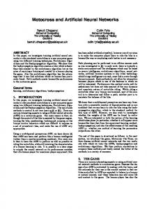
3. SPIKING NEURAL NETWORK 3.1 Architecture of Spiking Neural Network In this subsection, we briefly review the architecture of a spiking neural network and the temporally encoding of real input data. A spiking neural network is a one layer feed-forward neural network. We chose the simplest spike response model (SRM) as shown in Figure 1(a). In order to simplify the model and make it easy to understand, we assumed that before a neuron generates a spike, it has been at its resting state for a sufficiently long time so that the back propagation action potential is negligible. Also, in one learning cycle, the spike neuron can fire at most once. Therefore, the
electrical membrane potential of a post-synaptic neuron is the linear weighted combination of the kernel function ε (s ) which models the spike response to the pre-synaptic spikes. The weights indicate the efficacy of each synapse. When the membrane potential is over the threshold, the neuron will fire a spike, and then be reset to its resting potential.
(a) Simplified SRM Model.
(b) Enlargement of Each Connection
Figure 1 Architecture of Delayed Spiking Neural Network
Figure 2 and Equation (1) represents one of the most popular mathematical spike response models.
⎧s / τ exp(1 − s / τ ) ⎩ no response
ε ( s) = ⎨
if s > 0
(1)
else
Epsion Function 1
Membrane Potential
0.8
0.6
0.4
0.2
0 -5
0
5
10
15
20
Time [ms]
Figure 2 Spike Response Function, Post-synaptic Potential is Excitatory (EPSP)
The internal state of a post-synaptic neuron can be described as in Equation (2), where M is the number of the presynaptic neurons. M
u j (t ) = ∑ wij ε (t − t i )
(2)
i =1
This spiking neural network is a delayed neural network as introduced by Natschläger for the unsupervised clustering in his work.3 Between each pair of pre-synaptic and post-synaptic neurons, there are multiple time delays for each connection advised by Hopfield.4 Figure 1 (b) is an enlargement of this connection. The delay indicates the difference
between the firing time of the pre-synaptic spike and the arrival time of the spike to the post-synaptic neuron. Each delay has its own synapse efficacy. Therefore the internal state of a post-synaptic neuron can be described as in Equation (3). M
u j (t ) =
T
∑∑ w ε (t − t k ij
i
−dk)
(3)
i =1 k =1
In order to encode the input patterns temporally we can limit the value of the input variables in a range [0, T] which is also referred to as the coding interval. The value of the delay for each connection is in the same range and the step increase is d
k +1
− d k = 1 . Then, each input pattern can be encoded with the firing time of the input neurons as
t i = T − xi . In this model, the number of the pre-synaptic neurons is the dimension of the input vector. Each postsynaptic neuron indicates one cluster of the input patterns. 3.2 System Identification Method
Our goal is that after the system identification (i.e. learning all the parameters in the model), the spiking neural network can do clustering by using the firing time of post-synaptic neurons associated with each input pattern. Each postsynaptic neuron represented one cluster and fires earlier than other post-synaptic neurons for input patterns belonging to this cluster. We adopted a winner-take-all approach for the post-synaptic neurons to make sure only one spiking neuron fires in each input pattern. For each input vector, as soon as a post-synaptic neuron generates a spike, all the others will be inhibited. Moreover, only the synapse efficacy related to this post-synaptic neuron just fired will be changed according to the learning algorithm. Here, we chose Hebbian Learning rule through Spike Timing-Dependent Plasticity (STDP) as our learning algorithm.5,6 This learning method, proposed by Donald Hebb in his book entitled “The Organization of Behavior'', is referred to hereafter as the “Hebb's Learning Rule". It is the earliest and simplest learning rule for a neural network. It can be simply stated as “ When an axon of cell A is near enough to excite a cell B and repeatedly or persistently takes place in firing it, some growth process or metabolic change takes place in one or both cells such that A’s efficiency, as one of the cells firing B, is increased”. 7 In our STDP learning method, we incorporated synaptic depression in order to weaken the synaptic efficacy where the pre-synaptic neuron fires after the post-synaptic neuron.
∆t
dk ti
t post
t pre
Figure 3 Time Chart for Spiking
In Equation (4), G represents a generalized learning equation, where
ti is the firing time of the pre-synaptic neuron,
k
t post is the firing time of the post-synaptic neuron and d is the delay time. Figure 3 is the time chart for the spiking neuron.
d k wij (t ) = G (t i , t post , d k ) dt
(4)
Pre-synaptic neuron emits a spike at t i with delay d k , the post-synaptic neuron receives the synapse at t pre = t i + d k and generates a spike at t post
Figure 4 Learning Function
W ( ∆t ) where ∆t = t post − t pre
Under the STDP rule (Figure 4), the synaptic efficacy tends to change in two directions, either toward zero or toward the maximum weight. 5 If the synapse occurs before the post-synaptic spike, it will be increased; otherwise, decreased.
⎧ A p exp(∆t / τ p ) if ∆t < 0 ⎫ W (∆t ) = ⎨ ⎬ , ⎩− Ad exp(∆t / τ d ) if ∆t > 0⎭
(5)
where ∆t = t i + d − t post , W (∆t ) is a general representation of how the connecting weight changes. In Equation (5), A p and
Ad are the maximum changes caused by strengthening or weakening synaptic efficacy in
every learning cycle. In our system identification, the learning window is asymmetric as in Bi’s work.8 It implies that τ p and τ d have different values. In this model, the asymmetric property is essential since τ p and τ d indicate the range of how synaptic efficacy’ strengthening or weakening takes place. STDP learning rule ensures that only those synapses that reach the post-synaptic neuron shortly before it emits a spike are greatly increased. Those synapses that reach it much earlier merely increase insignificantly or stay the same, and those that reach it after are decreased. Additionally, the range of the weights must be bounded; otherwise the model will not be stable. In order to constrain the weights, we can choose either “hard-bound” or “soft-bound” with certain saturation functions. After each learning cycle, only a few delays will obtain large weights, while most of them will be close to the minimum weight or stay the same. Therefore, for each spiking neuron, all the delays will be changed in different directions adapting to the properties of the input patterns that activated this neuron. These changes can preserve the properties of each data cluster for future use. The model was first tested in some simulation tests and obtained good results. 9 But we found that the basic spiking neural network could not perform well if the input dimension is too small. This suggests that the high dimensional data may be more appropriate to this network model. However, the remote sensing data only have 7 bands in total. We excluded band 6 in our analysis because of its relatively low resolution. Practically, the reflectance data may not be available for all bands in each recording. In order to study the classification performance of different band combinations, subsets of the 6 bands need to be tested. This could lead to the insufficient dimension problem for the network model. Here, we utilized the encoding method similar to the Gaussian mixture model in Figure 5. We used several overlapping Gaussian receptive fields to encode each input value to a vector 10, so the total dimension of the input vector is the sum of all the numbers of the input data multiplying the number of the Gaussians.
1
2
3
4
5
6
7
8
9
10
20
0
p P = {0,0,3,14,16,4,0,0,0,0} Figure 5 Encoding a Value to a Vector with Overlapping Gaussians
According to Figure 5, we could easily encode an input value to a vector. For example, we have an input value p (shown in the figure). The dashed line indicates its responses for all Gaussians. We assumed those responses which are below a predefined threshold are not going to fire in the spiking neural network. Therefore, it is relatively easy to get the encoded vector P = {0,0,3,14,16,4,0,0,0,0} for the input value p . The number of Gaussians is up to the necessity. The more Gaussians there are, the more expensive the computation will get, while they can provide more information with a low input dimension. We applied this encoding method to the remote sensing data. Here, we normalized the original data to the range [0, C] by using the following equation,
X jk = C ⋅
1≤7 i≤4 P8 64 X jk − min( X ik )
max( X ik ) − min( X ik ) 1424 3 1424 3 1≤ i ≤ P
,
(6)
1≤ i ≤ P
where k is the band number, P is the number of total samples, j is in the range {1,2, L , P} , and C is a positive constant. In order to show that this spiking neural network performs better, we compared their classification results with traditional K-means clustering method, and recently developed spectral clustering method. Table 2 shows the partial result with different unsupervised classifications. We can see that the spiking neural network, though not perfect, can partially classify the data. In the table, “Answer” represents the number for each class extracted from the samples. “Result” represents the number of samples that belong to this class. The shaded area shows the spiking neural network achieved a better classification than the other two methods.
4. COMPLEX-VALUED NRBF NEURAL NETWORK 4.1 NRBF neural network
RBF neural networks have a strong biological background. In the field of the brain cortex, local regulated and folded receptive field is the characteristic of the reflection of the brain. Based on this characteristic, Moody and Darken 11,12 proposed a new neural network structure, which is referred to as RBF neural network. Figure 6 shows the basic topological structure of RBF neural network.
Kmeans-band123457
Answer1
Answer2
Answer3
Answer4
Answer5
Result1
20
1
0
0
0
Result2
0
118
0
100
1
Result3
0
0
81
0
0
Result4
80
0
0
0
0
Result5
0
0
19
0
99
Spectral-band123457
Answer1
Answer2
Answer3
Answer4
Answer5
Result1
100
0
0
0
0
Result2
0
0
40
0
0
Result3
0
0
60
0
26
Result4
0
119
0
100
0
Result5
0
0
0
0
74
Spiking-Band123457
Answer1
Answer2
Answer3
Answer4
Answer5
SPIKE NEURON 0
99
0
0
3
0
SPIKE NEURON 1
0
0
95
0
0
SPIKE NEURON 2
0
0
5
0
72
SPIKE NEURON 3
0
49
0
97
0
SPIKE NEURON 4
1
70
0
0
28
Table 2 Partial Result of Three Techniques
Figure 6 Topological Structure of RBF Neural Networks
Based on the RBF neural network structure and the chosen radial basis function, if f l ( X j ) is the lth output of the output layer, and
φi ( X j )
is the output of ith radial basis function, then the whole network forms a mapping:
f l ( X j ) = ∑ λil φi (X j ) , Nr
(7)
i =1
where X
j
is an M-dimensional feature vector; Y j is the actual output vector corresponding to the input vector X j ;
N r is the number of the hidden units and λi l is the connection weight between the ith hidden unit and lth output unit. This weight shows the contribution of the hidden unit to the corresponding output unit. In some approaches, the output of the hidden layer is normalized by the sum of all the radial basis function components just as in the Gaussian-mixtures estimation model.13 The following equation shows the normalized radial basis functions:
Φi ( X ) =
φi ( X − c i
)
∑i =1φi ( X − ci Nr
(8)
)
A network obtained using the normalized form for the basis functions is called a normalized RBF neural network (NRBF) and has some important properties. This normalized form bounds the hidden output in the range between 0 and 1, which can be interpreted as probability values to indicate which hidden units is most activated in classification application.14 Moreover, we modified the localized behavior to non-localized behavior which provides the right decision to all input vectors with this normalization. Using the above normalized form, we let f l ( X j ) be the lth output of the output layer, and Φ i ( X j ) be the normalized radial basis functions. Therefore, the equation (1) can be changed to the following one:
f l ( X j ) = ∑ λil Φ i (X j ) Nr
(9)
i =1
4.2 Complex-valued NRBF neural network
Here, we demonstrate that the complex-valued NRBF neural network can be applied to the classification of the remote sensing data. As in paper 1, the output of each class is the listed Table 3: Class Vegetation Soil (sparse vegetation) Urban area Deep water Shallow water
Output 1 0 0 0 0 1 0 0 0 0 1 0 0 0 0 1 0 0 0 0
0 0 0 0 1
Table 3 Output Table of Each Class
An advantage of the complex-valued NRBF network is that the output of the hidden layer is always a positive number. Since we have normalized the input vector, the input vector is always within the range [0, 1]. As for the output, since we used the definition as in Table 3, it is more appropriate to use the magnitude of the output from the hidden layer to represent the output of the network. It is necessary to add another activation function in the output layer as in Figure 7.
φ Re(λ1) Im(λ1)
Re(x1)+iIm(x1) Re(x2)+iIm(x2)
φ
Re(λ2) Im(λ2)
Re(λNr) Im(λNr) Re(xM)+iIm(xM)
∑ Re( f (X)) | |
∑ Im( f (X))
φ Figure 7 Schematic of Improved Complex-valued NRBFNN
g( X ) = f ( X )
The first stage of the complex-valued training is the same as the tradition NRBF neural network. In our experiments, the k-means clustering method was tested at this stage. Gaussian functions are fast decaying functions so that not all basis function units contribute significantly to the network output. In our work, they were used as the radius basis function (RBF). After the output of the hidden units is obtained, only the connecting weights between the hidden layer and the output layer should be trained. This modification of the structure changed the linear relationship between the hidden layer and the output layer to non-linear.
{X
Assume we have a group of input vectors
P
| X P ∈ C N , P = 1,2, L K
}
and their mappings are real
values {Y P | Y P ∈ R, P = 1,2, L K } , where N is the dimension of the input vector. We defined the following energy function as error function: E=
1 2
K
∑ (Y
P
P =1
− f(XP) )2 ,
(10)
where f ( X P ) is the output from the network of each corresponding input vector X P . As we have discussed, a variable in the complex domain includes a magnitude and a phase. In the complex-valued NRBF neural network, the normalized output of the hidden units for each input vector X P can be denoted as follows (for general use, we keep the hidden output in a complex-valued formula in case it is necessary to use the complex-valued number in the hidden layer. ): Φ M ( X P ) = λMP eiϕ MP (11)
Additionally, the weights between the hidden layer and the output layer can be denoted as WM = eiθ M , where the magnitude of the weight is 1 because the output is usually normalized. This definition shows one advantage of the complex-valued weights because during the learning process, only the phase is changed. This implies that we do not need any boundary limitation rule for the weights which is necessary in real artificial neural network. Using the gradient descent method to minimize the error signal, we can change the phase of each connecting weight through derivation:
∆θ i = −η
∂(
∂E = −η ∂θ i
1 2
K
∑ (Y P =1
P
− f(XP) )2 ) (12)
∂θ i
From the architecture of NRBF neural network, we had the detailed expression of the output before using the activation function. N
f( X P ) =
∑
N
Φ M ( X P )WM =
M =1
∑
λMP eiϕ MP eiθ M =
M =1
where N is the number of the hidden unit in the network, and
η
N
∑λ
MP e
i (θ M +ϕ MP )
,
(13)
M =1
is the learning step. Expanding (13), we had (14)
N
f(XP) =
∑ (λ
M
cos(θ M + ϕ MP ) + iλ M sin(θ M + ϕ MP ))
(14)
M =1
Plugging (14) into (12), we had ∆θ i = −η Let
∂E ∂ 1 = −η { ∂θ i ∂θ i 2
N
K
∑ (Y P =1
P
− [
∑λ
M =1
N
M
cos(θ M + ϕ MP )] 2 +[
∑λ
M =1
M
sin(θ M + ϕ MP )] 2 ) 2 } .
(15)
N
Θ =[
∑λ
N
M
cos(θ M + ϕ MP )] 2 +[
M =1
∑λ
M
sin(θ M + ϕ MP )] 2 .
(16)
M =1
Substituting (16) in (15),
∆θ i = −η
∂E ∂ ⎧⎪ 1 = −η ⎨ ∂θ i ∂θ i ⎪⎩ 2 K
= −η
∑ (Y
P
− Θ)
P =1 K
=η
∑ (Y
P
− Θ)
P =1
K
∑ (Y
P
P =1
⎫⎪ − Θ)2 ⎬ ⎪⎭
∂ (Y P − Θ ) ∂θ i
,
(17)
∂ (Θ ) 2 Θ ∂θ i 1
where N
∂ (Θ ) = ∂θ i
∂ ([
∑
N
λ M cos(θ M + ϕ MP )] 2 +[
M =1
∂θ i
∑λ
M
sin(θ M + ϕ MP )] 2 )
M =1
N
=2
∑λ
N
cos(θ M + ϕ MP )[λ i (− sin(θ i + ϕ iP )] + 2
M
M =1
∑λ
M
sin(θ M + ϕ MP )[λ i cos(θ i + ϕ iP )]
M =1
(18) Finally, we had the following full expression formula for the change of phase for each connection weight: K
∆θ i = −η
YP − Θ ∂E =η × ∂θ i Θ P =1
∑
N
(
N
∑
λM cos(θ M + ϕ MP )λi (− sin(θi + ϕiP )) +
∑
YP − Θ
M =1 K
=η
P =1
∑λ
M
sin(θ M + ϕ MP )λi cos(θ i + ϕiP ))
M =1
Θ
λi (im( f ( X P ) ) cos(θi + ϕiP ) − re( f ( X P ) ) sin(θi + ϕiP ))
(19)
The least mean square error algorithm does not guarantee convergence to globally optimal network parameters. However, it does appear to converge to reasonable solutions in practice.
4.3 Simulation Results
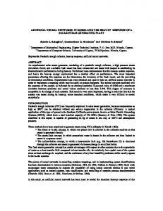
In this subsection, we explored this complex-valued NRBF model in the classification of the remote sensing data. We obtained the training and testing accuracy from both real-valued and the complex-valued NRBF neural networks. The results are listed in Table 4. Intuitively, we also showed them in Figure 8. Here, we compared the classification results of these two methods. We used the same collection of subsets of all the bands as the input for the neural networks. From Table 4, we can see that the complex weighted NRBF neural network can improve the classification result in most cases. Numerically, in the randomly selected 32 combinations, the complex-valued obtained higher accuracy in 21, and lower accuracy in 11. To statistically compare the results, we used the sign test by taking the null hypothesis Prob(the complex-valued method are more accurate) = 0.5. Under this hypothesis, we got p-value = 5.5x10⁻². The null hypothesis with such a low p-value should be rejected. This statistical result demonstrated that the complex-valued NRBF model performs significantly better than its real-valued counterpart. Note that for a few band combinations, for example, bands 2, 3 or bands 4, 5, 7, the complex-valued method even provided evidently higher classification accuracy.
100
95
) % ( y c ar u c c A
90
85
80 Complex-valued KmeansTesting Kmeans Testing 75
0
5
10
15 20 Test Times
25
30
Figure 8 Real-valued NRBF and Complex-valued NRBF
Table 4 Real-valued NRBF and Complex-valued NRBF
35
5. CONCLUSIONS
In this paper, we developed a collection of new clustering methods using several neural network models. These methods are focused on the practical applications of classification of remote sensing data. Our work focused on the classification of a satellite image of New England. This is a very important research field in environment management and protection. The distributions of all land coverage are very heterogeneous, and it is hard to study their properties under any parametric framework. In our work, we proposed to describe the distributions using these powerful artificial neural network models. We first described the development of a spiking neural network model which encodes the input data in temporal space. This is a new unsupervised classification technique. Using timing information, this model is a more biological accurate neural system than traditional artificial neurons. The parameters in the model were estimated using the STDP rule which is a robust learning method converged efficiently. We applied this spiking neural network to the classification of the remote sensing data. Experimental results showed that it can provide more useful information than traditional clustering methods. Secondly, we described the Complex-valued NRBF. The complexvalued NRBF neural network utilized the characteristics of complex numbers and represented the weights in the complex domain. We demonstrated that these complex weighted NRBF neural networks provided significant advantages in processing the remote sensing data. It not only kept the structure and efficiency of the NRBF neural network but also improved the computation power. This suggested that this new model is an efficient and effective method for classification of multi-spectral satellite image data. Our quantitative study showed that the proposed methods obtained more accurate classification than the traditional/existing methods. It can also overcome the computation complexity problem that has occurred in other work. 1 All these works can be directly applied to various research areas. They can also be implemented in other neural network structures.
REFERENCES
1. 2. 3. 4. 5. 6. 7. 8. 9. 10.
11. 12. 13. 14.
X.. Tao, and H. E. Michel, "Classification of Multi-spectral Satellite Image Data Using Improved NRBF Neural Networks," Proceedings of SPIE Vol. #5267-41, 2003. Robert A. Schowengerdt, Remote Sensing: Models and methods for image processing. Academic Press, 1997. T Natschläger, & B. Ruf (1998). “Spatial and temporal pattern analysis via spiking neurons,” Network: Computation in Neural Systems, 9(3): 319-332. J. J. Hopfield (1995). “Pattern recognition computation using action potential timing for stimulus representation,” Nature, 376:33-36. S. Song, K. D. Miller, & L. F. Abbott ( 2000). “Competitive Hebbian learning through spike timing-dependent synaptic plasticity,” Nature Neuroscience. 3:919-926. W Gerstner, & W. M. Kistler (2002). “Mathematical formulation of Hebbian learning,” Biological Cybernetics. 87:404-415. D. Hebb, (1949). The organization of behavior. New York: Wiley. G. Q. Bi, & M. M. Poo (1998). “Synaptic modifications in cultured hippocampal neurons: dependence on spiking timing, synaptic strength, and post synaptic cell type,” Journal of Neuroscience. 18:10464-10472. X.Tao, and H. E. Michel, "Data Clustering Via Spiking Neural Networks Through Spike Timing-Dependent Plasticity," Proceeding “IC-AI'04”, June 21-24, 2004, Las Vegas, Nevada, USA. S. M. Bohte, H. L. Poutre, and J. N. Kok (2002) ‘Unsupervised Clustering With Spiking Neurons by Sparse Temporal Coding and Multi Layer spike Neural Network’. IEEE Transactions on Neural Networks, Vol: 13 Issue: 2, March 2002 Page(s):426-435 Moody J, Darken C. “Fast Learning in Networks of Locally-turned Processing Units” Neural Computation, 1989 (1): 281-294, 1989. Moody J, Darken C. “Learning with localized Receptive Field” Proc 1988 Connectionist Models Summer school, Dtouretzky, G Hinton, and T Sejnowski(Eds.) Carnegie Mellon University, Morgan Kaufmann Publishers, 1988. Cha, I., Kassam, S. A. “ RBFN restoration of nonlinearly degraded images” IEEE Trans. On Image Processing, vol. 5, no. 6, pp. 964-975,1996. Robert J. Howlett and Lakhmi C. Jain. “Radial Basis Function Networks 1/2,” Physica-Verlag Heidelberg 2001.