NPClu: An Approach for Clustering Non-point Objects Maria Halkidi, Michalis Vazirgiannis Dept of Informatics, Athens University of Economics & Business, Greece Email:
[email protected],
[email protected]
Abstract. The vast majority of clustering algorithms and approaches deal with sets of objects, where objects are points in the multidimensional Euclidean space, each occupying zero hyper volume. There is a wealth of application domains that produce data sets in which the objects occupy hyperspace. Such application domains include spatiotemporal databases, medical applications etc. It is clear that clustering such data sets cannot be achieved by existing algorithms. In this paper we propose NPClu an approach for clustering sets of objects that are spatially extended. We experimentally evaluated the performance of our approach to show its effectiveness.
1
Introduction
Clustering is one of the most important data mining tasks. It aims at grouping objects into meaningful subclasses and identifying interesting distributions in the data under concern [3, 16]. A number of clustering algorithms have been proposed in the literature [1, 5, 6, 9, 10, 11, 13, 15, 16, 18]. To the best of our knowledge, the majority of them assume multidimensional point objects treating the issue of spatially extended objects insufficiently [12]. However, in many applications, such as spatio-temporal databases and medical applications, one would prefer searching for compact and well-separated groups of extended objects (e.g. line segments, polygons or volumes). A generalization of DBSCAN algorithm is presented in [19], aiming at clustering spatially extended objects. It relies on a density-based notion of clusters and is designed to discover arbitrarily shaped clusters. However, the quality of results depends on some user-defined density criteria, i.e. the neighborhood predicate that expresses the notion of neighborhood for the specific application and the cardinality function. Also, the distance function has to be defined properly depending on the application domain. An effort in [15] proposes a clustering method, termed WaveCluster, which aims at handling spatial databases. It exploits signal-processing techniques to convert the spatial data to the frequency domain and then finds dense regions in the new space. According to this approach an object may be represented by a feature vector (i.e. a point in n-dimensional space) and then clustering is applied to the feature space (instead of the objects themselves). It detects arbitrarily shaped clusters but it is not efficient in high dimensional spaces. Moreover, it is a complicated method based on the usage of signal processing techniques to represent data objects and find dense regions (clusters) in the data set.
Figure 1. Different approaches for clustering a set of 2D rectangles: (a) Set of rectangles – Dotted lines: Groups of rectangles(MBRs) (b) Clustering of MBRs’ centers In this paper the clustering requirement is to group objects that are more similar in terms of their distance and their structural properties (i.e. size) to the same cluster. We use the term real clusters to refer to the data groups that best reflect the real structure of data. These clusters correspond to the partitioning that we are expected to identify in a specific dataset. The partitioning that contains the real clusters is further called actual partitioning. Also we use the term correct number of clusters to refer to the number of clusters in the actual partitioning of a data set. Below we discuss in brief the non-point clustering problem and the need for introducing a new approach that addresses this problem. We use 2D examples for reasons of clarity but the approach applies to multidimensional cases as well. Problem Formulation. Figure 1a illustrates a set of rectangles. Rectangular shapes are popular in the spatial database literature; non-rectangular shapes can be approximated by their minimum bounding (hyper-) rectangles (MBRs) [4, 14]. The goal is to organize these rectangles into a set of clusters. Then the clustering problem can formally be defined as follows: Given a data set of n non-point objects, D, find a partitioning of D into groups (clusters) with respect to a similarity or distance measure. The partitioning should fulfill the properties: i) the members of a cluster have a high degree of similarity (i.e. are close to each other and have similar shape, size) and ii) the clusters themselves are widely spaced. A trivial solution in this case is to represent objects by their MBR centers. Then we can apply one of the well-known clustering algorithms proposed in the literature, such as BIRCH [18], CURE [9], DBSCAN [6] etc., to the extracted data set of objects’ centers. However, this mapping may ignore useful information about the original data set of objects leading to a clustering that does not fit the data well. This implies that the extracted clusters may not resemble the real clusters in the data set. To justify the above we consider the data set of non-point objects presented in Figure 1a. These objects are mapped to their MBRs’ centers and the resulting set is presented in Figure 1b. A clustering algorithm is applied to the set of centers partitioning it into four clusters. The solid lines in Figure 1b show the boundaries of the defined clusters. It is obvious that there are rectangles which are shared between clusters. This implies
that there is important information, regarding the real size of objects and their relative position (the position of an object with respect to others), which has been ignored. Comparing the clusters in Figure 1a with those in Figure 1b, we observe that based on the rectangles centers we don’t achieve to identify the real clusters in the dataset. The above motivates us to propose a new approach for Non-Point objects Clustering, called NPClu. It is based on representing objects by their MBRs’ vertices. The rest of the paper is organized as follows. In Section 2 we present the main steps of NPClu. Section 3 analyzes the fundamental step of the proposed method (i.e. refinement step), while it discusses integrity issues related to non-point clustering methodology. In Section 4, we present the experimental evaluation of NPClu. This is followed by an analysis of NPClu complexity. Finally, we conclude in Section 5.
2
The NPClu Algorithm
Our approach for clustering non-point data sets is based on three distinct steps: i) preprocessing, ii) clustering and iii) refinement. In the preprocessing step, the set of objects (e.g. rectangles) is represented in a ddimensional space by their MBRs’ vertices. Thus, a d-dimensional object is represented by 2d points in d-dimensional space. A set of points is defined that corresponds to the MBRs’ vertices of the initial set of objects, called transformed data set. Since we handle large spatial data sets, a R*-tree structure is built on the transformed data set1. The clustering step follows. One of the available clustering algorithms for points is applied to discover clusters of vertices in the transformed data set. This procedure results in a set of clusters where the vertices of a (hyper-) rectangle may be assigned to no cluster, or to a single cluster or to more than one clusters. As a consequence, there is a need for a refinement step. It elaborates on the initial clustering results and, using distance criteria, defines the final partitioning of the original set. More specifically, clusters may be merged and/or vertices may be moved from one cluster to another so that the vertices of a (hyper-) rectangle are classified into the same cluster. Furthermore, there are cases that some (hyper-) rectangles can be considered to be outliers/noise. Before discussing in detail the above methodology, we introduce some concepts that are fundamental in the context of the clustering and refinement phase. Definition 1: A rectangle2 (hyper-rectangle) R is defined to be resolved if all of its vertices are classified into the same cluster Ci. The vertices of R are called resolved vertices for the Ci. Definition 2: A rectangle R is defined as unresolved if its vertices are classified into different clusters.
1 We use the R*-tree since it is generally accepted as one of the most efficient R-tree variants. 2 In the context of this paper when we use the term rectangle we mean a hyper-rectangle.
Definition 3: Let x, y be two vertices of rectangle R. If the vertex x is classified into cluster Ci and y into Cj then x is defined to be an unresolved vertex of cluster Cj and y unresolved vertex of cluster Ci. Definition 4: Cluster size of the clusters Ci, further referred to as cluster_size(Ci), is calculated as the maximum distance between the vertices of all pairs of resolved rectangles in Ci. Definition 5: The intra-cluster distance of the Ci, intra_d(Ci), is defined as the minimum values of the following two distances: i) the average distance between the closest vertices of the resolved rectangles in Ci and ii) the average distance of the middle points of the rectangles’ edges. Definition 6: The relative connectivity between a pair of clusters Ci and Cj is defined as the number of unresolved rectangles between Ci and Cj normalized with respect to the number of resolved rectangles in Ci and Cj. Thus the relative connectivity between a pair of clusters Ci and Cj is given by Connectivity(C i , C j ) =
Unr _ rect Ci ∩ Unr _ rect C j
(Re s _ rect
Ci
+ Re s _ rect C j
)2
where Unr _ rect Ci ∩ Unr _ rect C j is the number of unresolved rectangles between Ci and Cj while Re s _ rect Ci is the number of resolved rectangles in Ci. Definition 7: Closeness of rectangle to clusters. Let Pi be an unresolved rectangle of clusters Ci and Cj. We also assume its nearest neighbors neigh_ci and neigh_cj in the clusters Ci and Cj respectively. Then, Pi is considered to be near both Ci and Cj if dci< max(intra_dCi, intra_dCj) and dCj< max(intra_dCi, intra_dCj), where intra_dCi, intra_dCj is the intra-cluster distance of Ci and Cj respectively and dCi, dCj is the distance of Pi from its nearest neighbor in cluster Ci and Cj respectively. The main steps of NPClu are discussed in detail in the following sections.
2.1 Preprocessing step The algorithm starts with the preprocessing phase in which the basic structures, used in clustering phase, are built. It includes two steps: • Mapping: Let Sobj be a set of (non-point) objects. A mapping of objects to their MBR vertices results in a transformed data set of rectangles, Svert. Each object is represented by the 2d vertices of its MBR: Svert = {(Pi(x1,…, xd), Pi)| Pi ∈ Sobj} where Pi(x1,…, xd) is a vertex of the MBR(Pi). Obviously, |Svert| = 2d⋅|Sobj|. • Building a R*-tree: We build a R*-tree [2] for the set of rectangles’ vertices, further called R(Svert). This is used by the following clustering step in order to find the nearest neighbors of a rectangle. Since R(Svert) is an index of points, its nodes at the leaf level consist of entries of the following structure: entry = {id, coordinates, cluster_id}, where id = {rect_id, vertex_id}, 0 ≤ vertex_id ≤ 2d-1, coordinates = (x1,…, xd) and cluster_id is a value to be assigned later (in the clustering step that follows).
2.2 Clustering step Once the set of vertices and the corresponding R*-tree are constructed, we proceed with the clustering phase. Actually, we apply a clustering algorithm to Svert, which discovers arbitrarily shaped clusters in underlying data and handles Figure 2. Defining noise in Case 2 and Case3 of the efficiently the outliers refinement step (DBSCAN is a good example of such an algorithm). Once clustering has been completed, we are aware of i) the clusters into which each of the rectangles’ vertices Pi(x1,…, xd) is classified and ii) the vertices defined as outliers/noise. Based on this information, R(Svert) is also properly updated, i.e. cluster_id value is defined. Clearly, after the clustering step we have only an indication of the objects’ classification since the corresponding vertices may have been classified into different clusters, some or all of them may have been defined as noise, etc. Thus, a refinement step is necessary to deal with the different cases of this problem and define the final partitioning of the underlying set of rectangles.
2.3 Refinement step Let C={Ci, i=1, …, numc} be the set of clusters defined during the clustering step. Then the main tasks of the refinement step are as follows: 1. For each Ci, we find: i. the rectangles whose all vertices are classified to the same cluster. Thus the set of resolved rectangles of Ci is defined (see Definition 1), Res_rectCi. For instance, in Figure 2 rectangle R3 is a resolved rectangle of cluster C1, ii. the rectangles whose vertices are classified to more than one clusters. The vertices of these rectangles define the set of unresolved rectangles of the cluster (see Definition 2), Unr_rectci. In Figure 2 the rectangle R1 is considered to be unresolved for clusters C1 and C2. iii. the vertices of rectangles that are considered to be noise/outlier define the set of noise for Ci (e.g. rectangle R4 is considered to be noise in the set presented in Figure 2). 2. The cluster size (see Definition 4) of each of the clusters in Ci∈C is defined based on Res_rectCi. Also, the intra-cluster distance (see Definition 5) of the clusters in C, intra_d(Ci) is defined. In case that there are no resolved rectangles in a cluster, we consider the MBR of the vertices that belong to this cluster. In this case only, both the intra-cluster distance and the size of the cluster are defined to be the longer edge of this MBR.
3
Finding the clusters of objects
Based on the above definitions and some distance criteria (as discussed below) we proceed to define the final partitioning of the set of rectangles. The clusters are merged or rectangles are moved from one cluster to another so that rectangles whose vertices split into different clusters are classified into the same cluster. Also, the outliers can be discovered and handled efficiently. In the context of this paper we only considered distance criteria in order to handle the outliers. However there are cases in which it is important to handle noise/outliers based on some other criteria that are not strictly related to the geometrical characteristics of objects. Hence we make the following assumption with regard to the definition of noise/outliers: If the length of unresolved rectangles is significantly higher than the average length of resolved rectangles then in addition to distance criteria we take into account non-spatial attributes of the objects so that the outliers are efficiently handled. In this section, however, we discuss the case that only the geometrical characteristics of objects are considered. More specifically, we consider the following cases of the problem regarding the classification of a rectangle: CASE 1. All the vertices of a rectangle are defined as noise. In this case the rectangle is also considered as noise. CASE 2. Only one cluster is involved in clustering results. We may consider the following two sub-cases: i. All the rectangle vertices are classified in a cluster. In this case, the rectangle is considered to be resolved and it belongs to the cluster of their vertices. ii. At least one of the rectangle’s vertices is defined as noise and the rest belong to the same cluster, C. Thus we have to decide whether R is noise or it has to be classified to C. To make a decision about R’s classification, we consider that the rectangle R is assigned in the cluster C (i.e. C Å C∪R) and then we compare the cluster size and intra-cluster distance of C before assigning R to C with the respective ones after the assignment. If there is significant change then R is defined to be noise otherwise is classified to C. Specifically the following procedure is applied: If | intra_d(C) – intra_d(C∪R)| > e then R is noise Else If | cluster_size(C) - cluster_size(C∪R) | > e then {R is noise Else Assign R to C}
The goal is to eliminate the possibility of destroying the homogeneity of a cluster, Ci, assigning to it an object that is not close or similar enough to the others classified in Ci. Assume for instance the rectangle R2 in Figure 2. Two of the R2’s vertices are assigned to C3 while the other two are labeled as noise. Assigning R2’s to C3 both the intra-cluster distance (intra_d) and the cluster size (cluster_size) of the cluster is significantly changed. Then based on our approach R2 is considered to be noise.
CASE 3. More than one clusters are involved in clustering results. The rectangle vertices are classified into more than one clusters (2, 3, …, 2d clusters). In this case that the number of involved clusters, denoted cl_inv, is larger than one some of the rectangles may be considered to be noise. In order to decide where the rectangle (further referred to as unresolved rectangle) can finally be classified, we are based on some criteria related to the connectivity (see Definition 6) and closeness (see Definition 7) of rectangles to the clusters under concern. Actually for each pair of the involved clusters their relative connectivity is calculated. The lower is the connectivity between clusters the higher is our confidence that there is noise between them. Hence if the clusters’ connectivity is lower than a user-defined threshold, θ, we proceed to define the potential noise between clusters. We compare the cluster size with the length of the unresolved rectangles and if the maximum cluster_size among the involved clusters is smaller than rect_length, the unresolved rectangle is considered to be noise. These criteria aim to avoid merging sets of objects that are not similar enough and thus change significantly the homogeneity of clusters. For instance consider the set of objects, S, depicted in Figure 2 and let {C1, C2, C3} be the set of clusters defined for the vertices of the rectangles in S. Since R1 is close to both C1 and C2 one could decide to merge clusters. Then, however, we decide to merge clusters that are not highly connected. The objects of C1 are connected to ones of C2 only through the rectangle R1 (low connectivity between C1 and C2). Moreover, comparing R1 with the sets of objects classified in C1 and C2 we observe that the assignment of R1 to the clusters can destroy the homogeneity of the clusters under concern. The length of R1 is higher than the size of C1 and C2. Thus we decide to label R1 as noise and define two well-separated and compact clusters. Thus the clusters C′1 and C′2 are defined as the dotted lines in Figure2 depict. On the other hand, if the connectivity between a pair of clusters is lower than a threshold, θ>0, the closeness of the unresolved rectangles to clusters is assessed in order to make the final decision for the unresolved clusters. Specifically, for each pair of the involved clusters (Ci, Cj) we compare the distance of the Ci′s (Cj′s) unresolved rectangle from its nearest neighbors in Ci(Cj) respectively with the maximum intra_cluster distance of the considered clusters. Based on the results of this comparison, we decide to merge the clusters or assign the unresolved rectangle to one of the involved clusters. The main procedure of this case can be summarized as follows: For i=1 to cl_inv For j=i+1 to cl_inv If (Connectivity(Ci, Cj) < θ) and (maxi=1,…,cl_inv(cluster_size)< rect_length) then Rectangle is noise Else { If (Connectivity (Ci, Cj) > θ) and (rectangle is near more than one cluster (see Definition 7)) then Merge these clusters else Assign rectangle to its nearest Cluster}
We note that the clustering process starts with the clusters that have the highest connectivity so as to result more effectively in a number of clusters with resolved rectangles and handle efficiently the noise/outliers.
(a) Before refinement step (b)After refinement step Figure 3. Applying NPClu to a set of rectangles in 3D-space.
The refinement procedure is iterative. It is repeated until there are no unresolved rectangles, that is, the algorithm terminates when all rectangles of the underlying set have been classified or have been defined as noise.
3.1
Integrity issues
One would argue that the NPClu methodology, especially the refinement step, needs some appropriate checking so that this step does not violate the integrity of the results provided by the clustering step. Below we analyze how NPClu treats different cases of the initial clustering results so as to define the final partitioning of a data set. Case 1: If NPClu clustering step discovers the actual partitioning of the data set, the refinement step does not change the partitioning. In this case the clustering algorithm partitions the data set of rectangles into the correct number clusters (as defined in the Introduction) that is all the vertices of a rectangle belong into the same cluster. Since there are no unresolved rectangles the refinement step is not applied. The output of NPClu is identical to the clustering step. Case 2: If NPClu clustering step discovers more clusters than the real ones, then the refinement step discovers the actual partitioning of the data set of rectangles. Assume that the clustering step partitions the transformed data set of rectangles (data set of vertices) into more than the correct number of clusters that appear in the data set of rectangles. Then, there are rectangles that are shared between two or more clusters and the refinement step is applied. The clusters are merged or rectangles are moved from one cluster to another so that the set of clusters in which the set of rectangles can be partitioned is defined.
4
NPClu Evaluation
In this section we discuss the results of our experimental study showing the effectiveness of our approach. The implementation of NPClu, described in Section 3,
(a) DS2 : Set of rectangles – Solid lines: NPClu results after the refinement step. (Noise:0%)
(b) Clustering on centers of rectangles- Naïve clustering
c) NPClu - Dotted lines show the boundaries of the clusters in the set of the rectangles’ vertices. Figure 4. The refinement step of NPClu is applied to define the final set of rectagles’clusters
is in C++. In the experiments we used DBSCAN [6] at the first clustering step of NPClu, and the implementation of R*-tree as presented in [2]. We chose DBSCAN since it is a widely used density-based algorithm that combines our requirements for clustering: i) discovery of arbitrarily shaped clusters, and ii) efficiency on large databases. Nevertheless, any other clustering algorithm can be used to discover significant groups in the set of rectangles’ vertices. NPClu uses the clustering algorithm only to define the initial set of clusters on which the main step of defining clusters into the set of objects (i.e. the refinement step) is based.
4.1 Experimental evaluation We experimented with several synthetic and real data sets in order to evaluate the performance of the proposed methodology for non-point objects clustering. Due to lack of space, we only give preliminary results here. Specifically, we use three data sets, which represent different cases of the refinement step (merge clusters, move objects between clusters, define rectangles as noise). Also we evaluate our approach using sets of rectangles with arbitrarily shaped clusters. They were defined based on a data set that is presented in [6]. Below we select to report our experimental results using two and three-dimensional datasets since they are more easily visualized. We note, however, that we obtained similar results with high-dimensional datasets.
a) DS3: Set of rectangles - Solid lines: NPClu clustering results after the refinement step (Noise: 1.5%)
b) Clustering on the centers of rectangles Naïve clustering
c) NPClu - Partitioning on the vertices of rectangles. The rectangles R4, R3 are unresolved. Figure 5. The refinement step of NPClu is required to define the final clusters
4.2 Discussion on the experimental results We assume a set of rectangles, further referred to as DS1, in 3D space presented in Figure 3a. One can observe two groups of rectangles (clusters) in DS1 while there is a rectangle that can be classified to both clusters. Figure 3a show the partitions defined on the set of rectangles’ vertices as defined using DBSCAN. It is obvious that there is a rectangle, R, that is unresolved and thus the refinement step is not applied. Then NPClu partitions DS1 into two clusters as Figure 3b shows while it defines the rectangle R to be noise. The following two experiments show the effectiveness of our approach in comparison with the naive approach. Figure 4a presents a data set of rectangles (further referred to as DS2), which, according to the clustering criteria introduced in previous sections, can be partitioned into 3 clusters. The mapping of rectangles to their centers is presented in Figure 4b. We apply DBSCAN to the set of rectangles’ centers and the resulting partitioning is a set of four clusters as the dotted lines show in Figure 4b. It is clear that the naïve approach does not work properly in this case. Then we consider the set of rectangles’ vertices, RV, and we run DBSCAN on it. Figure 4c shows the clusters that DBSCAN defined for RV. It is obvious that there is a set of unresolved
Figure 7. Centers of the rectangles presented in Figure 6
(a) Rectangle’s edge =0.2
rectangles. Thus, the refinement step is applied to define the final clusters in DS2. The lines in Figure 4a indicate the boundaries of the clusters defined by NPClu. It is obvious that NPClu achieves to identify the actual partitioning for DS2. A similar experiment is presented in Figure 5. Figure 5b depicts the set of rectangles, DS3, representing by their centers as (b) Rectangle’s edge =2 well as how this set can be Figure 6. Sets of rectangles with centers the partitioned by DBSCAN. On the points in Figure 7- The Lines indicates the other hand, the lines in Figure 5c clusters defined by NPClu show the clusters defined when DBSCAN run on the vertices of the rectangles in DS3 while Figure 5c depicts the final partitioning of DS3 as defined by NPClu. In this case the final sets of clusters is defined if we consider the initial partitioning of DBSCAN (as presented by dotted lines in Figure 5c) and then the unresolved rectangles (i.e., R4 and R3) are moved to the suitable cluster during the refinement step. The role of the geometrical characteristics in clustering. The following experiments show that NPClu works well in the case of arbitrarily shaped clusters of non-point (i.e. spatially extended) objects. Moreover, we show that our approach works as good as the approach based on centers when we consider a data set of small rectangles almost zero-point sized (see Figure 6a). In case that the data set consists of larger rectangles, moreover prolonged in one of their dimensions, our approach results in better partitioning since the rectangles’ centers cannot successfully represent them. Figure 7 depicts a set of data points considered in the following study to be the centers
based on which two sets of rectangles are defined (see Figure 6). The lines in Figure 7 show the partitioning of the data set as defined by DBSCAN. Assuming the set of points in Figure 7 to represent rectangles’ centers, we define the set of rectangles presented in Figure 6a. The partitioning defined by NPClu is represented by the lines in Figure 6a. Comparing the clusters depicted in Figure 7 and Figure 6a we observe that NPClu discovers the correct number of clusters as good as the approach based on the rectangles’ centers. Moreover we define a set of rectangles based on the same centers (presented in Figure 7) to the ones of rectangles in Figure 6a, but with larger edge. Then, the set of rectangles that Figure 6b shows is generated. It is clear that one can identify three well-separated clusters. Obviously, if we map the rectangles into their centers and we apply a clustering algorithm to the respective set of centers (i.e. the set of Figure 7), the set of four clusters presented in Figure 7 will be defined. On the other hand, considering the set of the rectangle vertices and applying NPClu, the expected set of clusters corresponding to the real clusters (as defined in the Introduction) is extracted. The lines in Figure 6b show the final set of clusters defined by NPClu. The above experimental study shows that NPClu achieves to find the real clusters presented in a set of objects taking into account different aspects of their geometrical structure (relative position, size).
4.3 Complexity issues The complexity of our approach is based on the complexity of the three steps described in Section 2, that is, the preprocessing, the clustering and the refinement step. The complexity of the first step is related to the mapping of objects to their MBR vertices and construction of the R*-tree, complexity O(2dn⋅log(2dn)), where n the number of rectangles and d is the dimension of the considered objects. The second step, which aims at discovering significant groups in the set of vertices, depends on the complexity of considered clustering algorithm. For example the complexity of DBSCAN is O(2dn⋅log(2dn)). Usually 2d