CWP-587P GEOPHYSICS, VOL. 73, NO. 5 共SEPTEMBER-OCTOBER 2008兲; P. VE145–VE159, 15 FIGS., 1 TABLE. 10.1190/1.2953337
Numeric implementation of wave-equation migration velocity analysis operators
Paul Sava1 and Ioan Vlad2
ABSTRACT Wave-equation migration velocity analysis 共MVA兲 is a technique similar to wave-equation tomography because it is designed to update velocity models using information derived from full seismic wavefields. On the other hand, wave-equation MVA is similar to conventional, traveltime-based MVA because it derives the information used for model updates from properties of migrated images, e.g., focusing and moveout. The main motivation for using wave-equation MVA is derived from its consistency with the corresponding wave-equation migration, which makes this technique robust and capable of handling multipathing characterizing media with large and sharp velocity contrasts. The wave-equation MVA operators are constructed using linearizations of conventional wavefield extrapolation operators, assuming small perturbations relative to the background velocity model. Similar to typical wavefield extrapolation operators, the wave-equation MVA operators can be implemented in the mixed space-wavenumber domain using approximations of different
INTRODUCTION Accurate wave-equation depth imaging requires accurate knowledge of a velocity model. The velocity model is used in the process of wavefield reconstruction, irrespective of the method used to solve the acoustic wave-equation, e.g., by integral methods 共Kirchhoff migration兲 or by differential/spectral methods 共migration by wavefield extrapolation and reverse-time migration兲. Generally speaking, there are two possible strategies for velocity estimation from surface seismic data in the context of wavefield depth migration. The two strategies differ by the domain in which the information used to update the velocity model is collected. The first strategy is formulated in the data space prior to migration, and it
orders of accuracy. As for wave-equation migration, wave-equation MVA can be formulated in different imaging frameworks, depending on the type of data used and image optimization criteria. Examples of imaging frameworks correspond to zero-offset migration 共designed for imaging based on focusing properties of the image兲, survey-sinking migration 共designed for imaging based on moveout analysis using narrow-azimuth data兲, and shot-record migration 共also designed for imaging based on moveout analysis, but using wide-azimuth data兲. The wave-equation MVA operators formulated for the various imaging frameworks are similar because they share elements derived from linearizations of the single square-root equation. Such operators represent the core of iterative velocity estimation based on diffraction focusing or semblance analysis, and their applicability in practice requires efficient and accurate implementation. This tutorial concentrates strictly on the numeric implementation of those operators and not on their use for iterative migration velocity analysis.
involves matching of recorded and simulated data using an approximate 共background兲 velocity model. Techniques in this category are known by the name of tomography 共or inversion兲. The second strategy is formulated in the image space after migration, and it involves measuring and correcting image features that indicate model inaccuracies. Techniques in this category are known as migration velocity analysis 共MVA兲 because they involve migrated images and not directly the recorded data. Tomography and migration velocity analysis can be implemented in various ways that can be classified based on the carrier of information from the data or image to the velocity model. Thus, we can distinguish between ray-based methods and wave-based methods. The terminology is applicable to both tomography and migration velocity analysis.
Manuscript received by the Editor 10 December 2007; revised manuscript received 12 March 2008; published online 1 October 2008. 1 Colorado School of Mines, Golden, Colorado, U.S.A. E-mail:
[email protected]. 2 StatoilHydro, Trondheim, Norway. E-mail:
[email protected]. © 2008 Society of Exploration Geophysicists. All rights reserved.
VE145
VE146
Sava and Vlad
For ray-based methods, the carrier of information consists of wide-band rays that are traced using a background velocity model from picked events in the data 共or image兲. Methods in this category are known as traveltime tomography 共Bishop et al., 1985兲 and traveltime MVA, sometimes described as image-space traveltime tomography 共Stork, 1992; al-Yahya, 1987; Fowler, 1988; Etgen, 1990; Chavent and Jacewitz, 1995; Clement et al., 2001; Chauris et al., 2002a, 2002b; Billette et al., 2003; Lambare et al., 2004; Clapp et al., 2004兲. For wave-based methods, the carrier of information consists of band-limited wavefields that are constructed using a background velocity model. Methods in this category are known as wave-equation tomography 共Gauthier et al., 1986; Tarantola, 1987; Mora, 1989; Woodward, 1992; Pratt, 1999, 2004兲 and wave-equation MVA 共Biondi and Sava, 1999; Sava and Biondi, 2004a, 2004b; Shen et al., 2005; Albertin et al., 2006b; Maharramov and Albertin, 2007兲. This paper concentrates on methods from the latter category. The volume of information used for model updates using wavebased methods is at least one order of magnitude larger than the volume of information used for ray-based methods. Thus we should ask a fundamental question: What is gained by using wave-based methods over ray-based methods? First, modern imaging applications using wave-based methods 共downward continuation or reverse-time extrapolation兲 require consistent velocity-estimation methods that interact with models in the same frequency band as the migration methods. Second, wavebased methods are robust 共i.e., stable兲 for models with large and sharp velocity variations 共e.g., salt兲. Third, wave-based methods describe naturally all propagation paths; thus, they easily can handle multipathing characterizing wave propagation in media with large velocity variations. Wave-equation tomography and wave-equation MVA have similarities and differences. In wave-equation tomography, the residual used for velocity updating is obtained by a direct comparison between recorded and measured data. In contrast, in wave-equation MVA the residual used for velocity updating is obtained by a comparison between a reference image and an improved version of it. On the other hand, wave-equation tomography has the disadvantage that the kinematics of events in the data domain are more complex than in the image domain. In addition, the dimensionality of the space in which to evaluate the misfit between recorded and simulated data is higher, potentially making a comparison more complex. Wave-equation MVAoptimizes directly the desired end product, i.e., the migrated image, which potentially makes this technique more “interpretive” and less of a computational “black box.” One important component of MVA methods is the type of measurement performed on migrated images to evaluate their imperfections. We can describe two kinds of information that, although strictly related to each other, are available to quantify image quality. The first kind is focusing analysis, which evaluates whether point-like events, e.g., fault truncations, are focused in migrated images at their correct positions. Image enhancement for wave-equation MVA can be formulated purely based on this type of information, which makes the techniques fast because they operate only with zero-offset data 共Sava et al., 2005.兲 The second kind of information is moveout analysis, which is the case for all conventional MVA techniques whether using rays or waves. In this case, we can formulate wave-equation MVA based on analysis of moveout of common-image gathers using velocity scans 共Biondi and Sava, 1999; Sava and Biondi, 2004a, 2004b; Soubaras
and Gratacos, 2007兲 or based on analysis of differential semblance of nearby traces in similar common-image gathers 共Shen et al., 2005兲. Moveout analysis requires construction of common-image gathers 共CIGs兲 characterizing the dependence of reflectivity function of various parameters used to parameterize multiple experiments used for imaging. There are two main alternatives for common-imagegather construction. First, we can construct offset-domain CIGs 共Yilmaz and Chambers, 1984兲 when reflectivity depends on sourcereceiver offset on the acquisition surface, which is a data parameter. Second, we can construct angle-domain CIGs 共de Bruin et al., 1990; Prucha et al., 1999; Mosher and Foster, 2000; Rickett and Sava, 2002; Xie and Wu, 2002; Sava and Fomel, 2003; Soubaras, 2003; Fomel, 2004; Biondi and Symes, 2004兲 when reflectivity depends on the angles of incidence at the reflection point, which is an image parameter. For wave-equation migration, offset-domain CIGs are not a practical solution because the information from multiple offsets 共or multiple seismic experiments兲 mixes in the process of migration. Furthermore, angle-domain CIGs suffer from fewer artifacts than offset-domain CIGs because angle-gathers are parameterized relative to image coordinates 共after wavefield reconstruction兲, as opposed to offset-gathers that are parameterized relative to data coordinates 共before wavefield reconstruction兲 共Stolk and Symes, 2004兲. Both wave-equation tomography and wave-equation MVA methods are based on a fundamental “small perturbation” assumption, which requires a reasonably good starting model. This requirement represents a drawback that is responsible for the main difficulty of methods in both categories. For wave-equation tomography or inversion, we can update models based on differences between recorded and simulated data. If the starting background model is not accurate enough, we run the risk of subtracting wavefields corresponding to different events. Likewise, for wave-equation MVA, we update the model based on differences between two images: one simulated in the background model and an enhanced version of this image. If the enhanced version of the image goes too far from the reference image, we run the risk of subtracting events corresponding to different reflectors. This phenomenon usually is referred to in the literature as “cycle skipping,” and various strategies are designed to ameliorate this problem, e.g., by optimal selection of frequencies used for velocity analysis 共Sirgue and Pratt, 2004; U. Albertin, personal communication, 2006兲. However, alternative methods used to evaluate image accuracy, e.g., differential semblance 共Symes and Carazzone, 1991; Shen et al., 2003兲, have the best potential to ameliorate this situation. In this case, wave-equation MVA analyzes the difference between image traces within common-image gathers, which are likely to be similar enough to avoid the cycle-skipping problem. Even in this case, the assumption is that the nearby traces in a gather are sampled well enough; i.e., the seismic events differ by only a fraction of the wavelet, which is a function of image sampling and frequency content. In practice, there is no absolute guarantee that nearby events are closely related to one another, although this is more likely to be true for differential semblance optimization 共DSO兲 than it is for direct-image differencing. In this paper, we concentrate on the implementation of the waveequation migration velocity analysis operators for various waveequation migration configurations. The main objective is to derive the linearized operators linking perturbations of the slowness model
Implementation of wave-equation MVA operators to the corresponding perturbations of the seismic wavefield and image. All theoretical development is formulated under the single scattering 共Born兲 approximation applied to acoustic waves. We begin by describing the MVA operators corresponding to zero-offset, survey-sinking, and shot-record wave-equation migration frameworks. We describe the theoretical background for each operator and emphasize the similarities and differences among the different operators. Throughout, we use pseudocode to illustrate implementation strategies and data flow for the various wave-equation MVA operators. Finally, we illustrate the wave-equation MVA operators with impulse responses corresponding to simple and complex models. We leave outside the scope of this paper the procedure in which the discussed operators are used for migration velocity analysis.
WAVE-EQUATION MIGRATION AND VELOCITY ANALYSIS OPERATORS The conceptual framework of wave-equation MVA is similar to that of conventional 共ray-based兲 MVA in that the source of information for velocity updating is extracted from features of migrated images. In contrast, with wave-equation tomography 共or inversion兲 the source of information is represented by the mismatch between recorded and simulated data. The main difference between waveequation MVA and ray-based MVA is that the carrier of information from the migrated images to the velocity model is represented by the entire extrapolated wavefield, and not by a ray field constructed from selected points in the image based on an approximate velocity model. The key element for the wave-equation MVA technique is a definition of an image perturbation corresponding to the difference between the image obtained with a known background velocity model and an improved image. Such image perturbations can be constructed using straight differences between images 共Biondi and Sava, 1999; Albertin et al., 2006a兲 or by examining moveout parameters in migrated images 共Sava and Biondi, 2004a, 2004b; Shen et al., 2005; Albertin et al., 2006b, Maharramov and Albertin, 2007兲. Then, using wave-equation MVA operators, the image perturbations can be translated into slowness perturbations, which update the model. The direct analogy between wave-based MVA and ray-based MVA is the following: Wave-based methods use image perturbations and back propagation using waves, while ray-based methods use traveltime perturbations and back propagation using rays. Thus, wave-equation MVA benefits from all the characteristics of wavebased imaging techniques, e.g., stability in areas of large velocity variation, while remaining conceptually similar to conventional traveltime-based MVA. We can formulate wave-equation migration and velocity analysis for different configurations in which we process the recorded data. There are two main classes of wave-equation migration: surveysinking migration and shot-record migration 共Claerbout, 1985兲, which differ in the way recorded data are processed. Both waveequation imaging techniques use similar algorithms for downward continuation and, in theory, produce identical images for identical implementation of extrapolation operators if all data are used for imaging 共Berkhout, 1982; Biondi, 2003兲. The main difference is that shot-record migration is used to process separate seismic experiments 共shots兲 sequentially, while survey-sinking migration is used to process all seismic experiments 共shots兲 simultaneously.
VE147
The shot-record operators are more computationally expensive but less memory intensive than the survey-sinking operators. A special case of survey-sinking migration assumes that the sources and receivers are coincident on the acquisition surface, a technique usually described as the exploding reflector model 共Loewenthal et al., 1976兲 applicable to zero-offset data. All operators described here can be used in models characterized by complex wave propagation 共multipathing兲. In all situations, wave-equation migration can be formulated as consisting of two main steps. The first step is wavefield reconstruction 共abbreviated w.r. for the rest of this paper兲 at all locations in space and using all frequencies from the recorded data as boundary conditions. This step requires numeric solutions to a form of wave equation, typically the one-way acoustic wave equation. The second step is the imaging condition 共abbreviated i.c. for the rest of this paper兲, which is used to extract from the reconstructed wavefield共s兲 the locations in which reflectors occur. This step requires numeric implementation of image-processing techniques, e.g., crosscorrelation, which evaluate properties of the wavefield indicating the presence of reflectors. Needless to say, the two steps are not implemented sequentially in practice because the size of the wavefield usually is large and cannot be handled efficiently on conventional computers. Instead, wavefield reconstruction and imaging condition are implemented on the fly, avoiding expensive data storage and retrieval. Wave-equation MVA requires implementation of an additional procedure that links image and slowness perturbations. This link is given by a wavefield-scattering operation 共abbreviated w.s. for the rest of this paper兲, which is derived by linearization from conventional wavefield-extrapolation operators. In the following sections, we describe the migration and velocity analysis operators for the various imaging configurations. We begin with zero-offset imaging under the exploding reflector model because this is the simplest wave-equation imaging framework, and it can aid our understanding of both survey-sinking and shot-record migration and velocity analysis frameworks. We continue with a description of the wave-equation migration velocity analysis operator for multioffset data using the survey-sinking and shot-record migration configuration. For each configuration, we describe the implementation of the forward operator 共used to translate model perturbations into image perturbations兲 and of the adjoint operator 共used to transform image perturbations into model perturbations兲. Both forward and adjoint operators are necessary for the implementation of efficient, numeric conjugate-gradient optimization 共Claerbout, 1985兲. Throughout this paper, we use the following notations and naming conventions:
: angular frequency z: depth coordinate m ⳱ 兵mx,my其: midpoint coordinates h ⳱ 兵hx,hy其: half-offset coordinates km ⳱ 兵kmx,kmy其: midpoint wavenumbers kh ⳱ 兵khx,khy其: half-offset wavenumbers s共m兲: medium slowness s0共m兲: background slowness u共m兲 or u共m,h兲: wavefield at frequency and depth z for zerooffset and multiple-offset data, respectively • ⌬u共m兲 or ⌬u共m,h兲: scattered wavefield at frequency and
• • • • • • • • •
VE148
Sava and Vlad
depth z for zero-offset and multiple-offset data, respectively • r共m兲 or r共m,h兲: image at depth z for zero-offset and multiple-offset data, respectively • i.c.: imaging condition • w.r.: wavefield reconstruction 共extrapolation兲 • w.s.: wavefield scattering • EⳲ关兴: extrapolation operator 共causal for ⫹, anticausal for ⫺兲 • FⳲ关兴: forward scattering operator 共causal for ⫹, anticausal for ⫺兲 • Am关兴: adjoint scattering operator 共causal for ⫹, anticausal for ⫺兲
Zero-offset migration and velocity analysis Wavefield reconstruction for zero-offset migration based on the one-way wave equation is performed by recursive phase shift in depth, starting with data recorded on the surface as boundary conditions. In this configuration, the imaging condition extracts the image as time t ⳱ 0 from the reconstructed wavefield at every location in space. Thus, the surface data need to be extrapolated backward in time, which is achieved by selecting the appropriate sign of the phase-shift operation 共which depends on the sign convention for temporal Fourier transforms兲,
uzⳭ⌬z共m兲 ⳱ eⳮikz⌬zuz共m兲.
共1兲
In equation 1, uz共m兲 represents the acoustic wavefield at depth z for a given frequency at all positions in space m, and uzⳭ⌬z共m兲 represents the same wavefield extrapolated to depth z Ⳮ ⌬z. The phaseshift operation uses the depth wavenumber kz, which is defined by the single square-root 共SSR兲 equation
kz ⳱ 冑关2 s共m兲兴2 ⳮ 兩km兩2 ,
共2兲
where s共m兲 represents the spatially variable slowness at depth level z. Equations 1 and 2 describe wavefield extrapolation using a pseudodifferential operator, which justifies the use of laterally varying slowness s共m兲. As indicated earlier, the image is obtained from this extrapolated wavefield by selection of time t ⳱ 0, which typically is implemented as summation of the extrapolated wavefield over frequencies,
rz共m兲 ⳱ 兺 uz共m, 兲.
共3兲
Phase-shift extrapolation using wavenumbers computed by using equations 1 and 2 is not feasible in media with lateral variation. Instead, implementation of such operators is done by using approximations implemented in a mixed space-wavenumber domain 共Stoffa et al., 1990; Ristow and Ruhl, 1994; Huang et al., 1999兲.Abrief summary of the mixed-domain implementation of the split-step Fourier 共SSF兲 operator is presented in Appendix A. For velocity analysis, we assume that we can separate the total slowness s共m兲 into a known background component s0共m兲 and an unknown component ⌬s共m兲. With this convention, we can linearize the depth wavenumber kz relative to the background slowness s0 using a truncated Taylor series expansion
kz ⬇ kz0 Ⳮ
冏 冏 dkz ds
⌬s共m兲,
共4兲
s0
where the depth wavenumber in the background medium characterized by slowness s0共m兲 is
kz0 ⳱ 冑关2 s0共m兲兴2 ⳮ 兩km兩2 .
共5兲
Here, s0共m兲 represents the spatially variable background slowness at depth level z. Using the wavenumber linearization from equation 4, we can reconstruct the acoustic wavefields in the background model using a phase-shift operation
uzⳭ⌬z共m兲 ⳱ eⳮikz0⌬zuz共m兲.
共6兲
We can represent wavefield extrapolation using a generic solution to the one-way wave equation using the notation uzⳭ⌬z共m兲 ⳱ Eⳮ ZOM 关2s 0z共m兲,u z共m兲兴. This notation indicates that the wavefield uzⳭ⌬z共m兲 is reconstructed from the wavefield uz共m兲 using the background slowness s0共m兲. This operation is repeated independently for all frequencies . A typical implementation of zero-offset wave-equation migration uses the following algorithm: ZERO-OFFSET MIGRATION ALGORITHM
ω = ωmin . . . ωmax { read u (m) z = zmin . . . zmax { @ z and ω (optional) write u (m) @z read r (m) i .c . r (m) + = u (m) @z write r (m) − w . r. u (m) = EZOM [2s0 (m) , u (m)] } } @ω
Aseismic image is produced using migration by wavefield extrapolation as follows: For each frequency, read data at all spatial locations m, then for each depth, sum the wavefield into the image at that depth level 共i.e., apply the imaging condition兲 and then reconstruct the wavefield to the next depth level 共i.e., perform wavefield extrapolation兲. The “⫺” sign in this algorithm indicates that extrapolation is anticausal 共backward in time兲, and the factor “2” indicates that we are imaging data recorded in two-way traveltime with an algorithm designed under the exploding reflector model. Wavefield extrapolation usually is implemented in a mixed domain 共space-wavenumber兲, as briefly summarized in Appendix A. The wavefield perturbation ⌬u共m兲 caused at depth z Ⳮ ⌬z by a slowness perturbation ⌬s共m兲 at depth z is obtained by subtraction of the wavefields extrapolated from z to z Ⳮ ⌬z in the true and background models,
⌬uzⳭ⌬z共m兲 ⳱ eⳮikz⌬zuz共m兲 ⳮ eⳮikz0⌬zuz共m兲 ⳱ eⳮikz0⌬z关eⳮi兩dkz /ds兩s0⌬s共m兲⌬z ⳮ 1兴uz共m兲.
共7兲
Here, ⌬u共m兲 and u共m兲 correspond to a given depth level z and frequency .Asimilar relation can be applied at all depths and at all frequencies. Equation 7 establishes a nonlinear relation between the wavefield perturbation ⌬u共m兲 and the slowness perturbation ⌬s共m兲. Given the complexity and cost of numeric optimization based on nonlinear relations between model and wavefield parameters, it is desirable to simplify this relation to a linear relation between model and data parameters. Assuming small slowness perturbations, i.e., small phase perturbations, the exponential function eⳲi兩 dkz / ds 兩s0⌬s共m兲⌬z can be linearized using the approximation ei ⬇ 1 Ⳮ i , which is valid for small values of the phase .
Implementation of wave-equation MVA operators Therefore, the wavefield perturbation ⌬u共m兲 at depth z can be written as
⌬u共m兲 ⬇ ⳮi
冏 冏 dkz ds
⬇ ⳮi⌬z
⌬zu共m兲⌬s共m兲 2
冑 冋
兩km兩 1ⳮ 2 s0共m兲
册
2
u共m兲⌬s共m兲. 共8兲
Equation 8 defines the zero-offset forward scattering operator Fⳮ ZOM 关u共m兲,2s 0共m兲,⌬s共m兲兴, producing the scattered wavefield ⌬u共m兲 from the slowness perturbation ⌬s共m兲, based on the background slowness s0共m兲 and background wavefield u共m兲 at a given frequency . The image perturbation at depth z is obtained from the scattered wavefield using the time t ⳱ 0 imaging condition, similar to the procedure used for imaging in the background medium,
⌬r共m兲 ⳱ 兺 ⌬u共m, 兲.
共9兲
Given an image perturbation ⌬r共m兲, we can construct the scattered wavefield by the adjoint of the imaging condition
⌬u共m, 兲 ⳱ ⌬r共m兲,
共10兲
for every frequency . Then the slowness perturbation at depth z and frequency caused by a wavefield perturbation at depth z under the influence of the background wavefield at the same depth z can be written as
⌬s共m兲 ⬇ Ⳮ i
冏 冏 dkz ds
⬇ Ⳮ i⌬z
ZERO-OFFSETADJOINT SCATTERING ALGORITHM @ω
s0
⌬zu共m兲⌬u共m兲 s0
2
冑 冋
兩km兩 1ⳮ 2 s共m兲
册
2
u共m兲⌬u共m兲.
共11兲
VE149
@ z and ω w. r. @z i. c . @z w. s. @z
ω = ωmin . . . ωmax { initialize ∆u (m) = 0 z = zmax . . . zmin { read u (m) + ∆u (m) = EZOM [2s0 (m) , ∆u (m)] read ∆r (m) ∆u (m) + = ∆r (m) read ∆s (m) + ∆s (m) + = AZOM [u (m) , 2s0 (m) , ∆u (m)] write ∆s (m) } }
The forward zero-offset wave-equation MVA operator follows a similar pattern to the implementation of the downward continuation operator: For each frequency and for each depth, read the slowness perturbation ⌬s at all spatial locations m. Next, apply the scattering operator w.s. given in equation 11 to the slowness perturbation and accumulate the scattered wavefield for downward continuation. Then apply the imaging condition i.c. producing the image perturbation ⌬r at depth z and reconstruct the scattered wavefield backward in time using the wavefield extrapolation operator w.r. to the next depth level. The adjoint zero-offset wave-equation MVA operator follows a similar pattern to the implementation of the downward continuation operator: For each frequency and for each depth, reconstruct the scattered wavefield forward in time using the wavefield extrapolation operator w.r. to the next depth level. Next, apply the adjoint of the imaging condition i.c. by adding the image to the scattered wavefield. Then apply the adjoint wavefield-scattering operator w.s. to obtain the slowness perturbation ⌬s. Both forward and adjoint scattering algorithms require the background wavefield, u, to be precomputed at all depth levels, although more efficient implementations using optimal checkpointing are possible 共Symes, 2007兲. Scattering and wavefield extrapolation are implemented in the mixed space-wavenumber domain, as briefly explained in Appendix A.
Equation 11 defines the adjoint scattering operator AⳭ ZOM 关u共m兲,2s0共m兲,⌬u共m兲兴, producing the slowness perturbation ⌬s共m兲 from the scattered wavefield ⌬u共m兲, based on the background slowness s0共m兲 and background wavefield u共m兲. A typical implementation of zero-offset forward and adjoint scattering uses the following algorithms:
Survey-sinking migration and velocity analysis
ZERO-OFFSET FORWARD SCATTERING ALGORITHM
followed by extraction of the image at time t ⳱ 0. Here, m and h stand for midpoint and half-offset coordinates, respectively, defined according to the relations
@ω @ z and ω @z w. s . @z i. c . @z w. r .
ω = ωmin . . . ωmax { initialize ∆u (m) = 0 z = zmin . . . zmax { read u (m) read ∆s (m) − ∆u (m) + = FZOM [u (m) , 2s0 (m) , ∆s (m)] read ∆r (m) ∆r (m) + = ∆u (m) write ∆r (m) − ∆u (m) = EZOM [2s0 (m) , ∆u (m)] } }
Wavefield reconstruction for multioffset migration based on the one-way wave equation under the survey-sinking framework 共Claerbout, 1985兲 is implemented similar to the zero-offset case by recursive phase shift of prestack wavefields
uzⳭ⌬z共m,h兲 ⳱ eⳮikz⌬zuz共m,h兲,
共12兲
m⳱
rⳭs 2
共13兲
h⳱
rⳮs , 2
共14兲
and
where s and r are coordinates of sources and receivers on the acquisition surface.
VE150
Sava and Vlad
In equation 12, uz共m,h兲 represents the acoustic wavefield for a given frequency at all midpoint positions m and half-offsets h at depth z, and uzⳭ⌬z共m,h兲 represents the same wavefield extrapolated to depth z Ⳮ ⌬z. The phase — shift operation uses the depth wavenumber kz, which is defined by the double square-root 共DSR兲 equation
k z ⳱ k zs Ⳮ k zr ⳱ Ⳮ
冑
冑
关 s共mⳮh兲兴2 ⳮ
关 s共mⳭh兲兴2 ⳮ
冏
冏
km Ⳮ kh 2
km ⳮ kh 2
冏
冏
2
2
共15兲
.
The image is obtained from this extrapolated wavefield by selection of time t ⳱ 0, which usually is implemented as summation over frequencies,
rz共m,h兲 ⳱ 兺 uz共m,h, 兲.
共16兲
Similar to the derivation done in the zero-offset case, we can assume the separation of the extrapolation slowness s共m兲 into a background component s0共m兲 and an unknown perturbation component ⌬s共m兲. Then we can construct a wavefield perturbation ⌬u共m,h兲 at depth z and frequency related linearly to the slowness perturbation ⌬s共m兲. Linearizing the depth wavenumber given by the DSR equation 15 relative to the background slowness s0共m兲, we obtain
kz ⬇ kz0 Ⳮ
冏 冏 dkzs ds
⌬s共mⳮh兲 Ⳮ s0
冏 冏 dkzr ds
⌬s共mⳭh兲, s0
SURVEY-SINKING MIGRATION ALGORITHM
ω = ωmin . . . ωmax { read u (m, h) z = zmin . . . zmax { @ z and ω (optional) write u (m, h) @z read r (m, h) i .c . r (m, h) + = u (m, h) @z write r (m, h) − w. r . u (m, h) = ESSM [s0 (m) , u (m, h)] } } @ω
This algorithm is similar to the one described in the preceding section for zero-offset migration, except that 共1兲 the wavefield and image are parameterized by midpoint and half-offset coordinates, and 共2兲 the depth wavenumber used in the extrapolation operator is given by the DSR equation using the background slowness s0共m兲. Wavefield extrapolation usually is implemented in a mixed-domain 共space-wavenumber兲, as briefly summarized in Appendix A. Similar to the derivation of the wavefield perturbation in the zerooffset migration case, we can write the linearized wavefield perturbation for survey-sinking migration as
⌬u共m,h兲 ⬇ ⳮi Ⳮ
冑 冑
冏
Ⳮ
关 s0共m Ⳮ h兲兴2 ⳮ
冏
冏
dkzr ds
⌬s共mⳮh兲 s0
冏
册
⌬s共mⳭh兲 ⌬zu共m,h兲 s0
冑 冋 1ⳮ
兩km ⳮ kh兩 2 s0共mⳮh兲
冑 冋 1ⳮ
2
.
共18兲
Here, s0共m兲 represents the spatially variable background slowness at depth level z. Using the wavenumber linearization given by equation 17, we can reconstruct the acoustic wavefields in the background model using a phase-shift operation
uzⳭ⌬z共m,h兲 ⳱ eⳮikz0⌬zuz共m,h兲.
冏 冏
ⳮi⌬z
2
km Ⳮ kh 2
ds
册
2
⫻u共m,h兲⌬s共mⳮh兲
where the depth wavenumber in the background medium is
kz0 ⳱
dkzs
⬇ ⳮi⌬z
共17兲
km ⳮ kh 关 s0共m ⳮ h兲兴2 ⳮ 2
冋冏 冏
共19兲
We can represent wavefield extrapolation using a generic solution to the one-way wave equation using the notation uzⳭ⌬z共m,h兲 ⳱ Eⳮ SSM 关s 0z共m兲,u z共m,h兲兴. This notation indicates that the wavefield uzⳭ⌬z共m,h兲 is reconstructed from the wavefield uz共m,h兲 using the background slowness s0共m兲. This operation is repeated independently for all frequencies . A typical implementation of survey-sinking wave-equation migration uses the following algorithm:
兩km Ⳮ kh兩 2 s0共mⳭh兲
⫻u共m,h兲⌬s共mⳭh兲.
册
2
共20兲
Equation 20 defines the forward scattering operator Fⳮ SSM 关u共m,h兲, s0共m兲,⌬s共m,h兲兴, producing the scattered wavefield ⌬u共m,h兲 from the slowness perturbation ⌬s共m兲, based on the background slowness s0共m兲 and background wavefield u共m,h兲. The image perturbation at depth z is obtained from the scattered wavefield using the time t ⳱ 0 imaging condition, similar to the procedure used for imaging in the background medium,
⌬r共m,h兲 ⳱ 兺 ⌬u共m,h, 兲.
共21兲
Given an image perturbation ⌬r共m,h兲, we can construct the scattered wavefield by the adjoint of the imaging condition
⌬u共m,h, 兲 ⳱ ⌬r共m,h兲, for every frequency .
共22兲
Implementation of wave-equation MVA operators Then, similar to the procedure used in the zero-offset case, the slowness perturbation at depth z caused by a wavefield perturbation at depth z under the influence of the background wavefield at the same depth z can be written as
⌬s共mⳮh兲 ⬇ Ⳮi
冏 冏 dkzs ds
⬇ Ⳮi⌬z
⌬zu共m,h兲⌬u共m,h兲 s0
冑 冋 1ⳮ
兩km ⳮ kh兩 2 s0共mⳮh兲
册
2
⫻u共m,h兲⌬u共m,h兲, and
⌬s共m Ⳮ h兲 ⬇ Ⳮi
冏 冏 dkzr ds
⬇ Ⳮi⌬z
Shot-record migration and velocity analysis 共23兲
⌬zu共m,h兲⌬u共m,h兲
冑 冋 1ⳮ
兩km Ⳮ kh兩 2 s0共mⳭh兲
⫻u共m,h兲⌬u共m,h兲.
册
共24兲
SURVEY-SINKING FORWARD SCATTERING ALGORITHM
@ z and ω @z w. s.(source) w.s .(receiver) @z i. c . @z w. r .
ω = ωmin . . . ωmax { initialize ∆u (m, h) = 0 z = zmin . . . zmax { read u (m, h) read ∆s (m) − [u (m, h) , s0 (m − h) , ∆s (m − h)] ∆u (m, h) + = FSSM − ∆u (m, h) + = FSSM [u (m, h) , s0 (m + h) , ∆s (m + h)] read ∆r (m, h) ∆r (m, h) + = ∆u (m, h) write ∆r (m, h) − ∆u (m, h) = ESSM [s0 (m) , ∆u (m, h)] } }
SURVEY–SINKING ADJOINT SCATTERING ALGORITHM @ω @ z and ω w. r . @z i. c . @z w.s .(source) w.s .(receiver) @z
Wavefield reconstruction for multioffset migration based on the one-way wave equation under the shot-record framework is performed by separate recursive extrapolation of the source and receiver wavefields, us and ur. The wavefield extrapolation progresses forward in time 共causal兲 for the source wavefield and backward in time 共anticausal兲 for the receiver wavefield,
uszⳭ⌬z共m兲 ⳱ eⳭikz⌬zusz共m兲
共25兲
urzⳭ⌬z共m兲 ⳱ eⳮikz⌬zurz共m兲.
共26兲
and
2
Equations 23 and 24 define the adjoint scattering operator AⳭ SSM 关u共m,h兲,s0共m兲,⌬u共m,h兲兴, producing the slowness perturbation ⌬s共m兲 from the scattered wavefield ⌬u共m,h兲, based on the background slowness s0共m兲 and background wavefield u共m,h兲. A typical implementation of survey-sinking forward and adjoint scattering follows the algorithms.
@ω
thermore, the two square roots corresponding to the DSR equation update the slowness model separately, thus characterizing the source and receiver propagation paths to the image positions. Both forward and adjoint scattering algorithms require the background wavefield, u共m,h兲, to be precomputed at all depth levels. Scattering and wavefield extrapolation are implemented in the mixed space-wavenumber domain, as briefly explained in Appendix A.
s0
VE151
ω = ωmin . . . ωmax { initialize ∆u (m, h) = 0 z = zmax . . . zmin { read u (m, h) + ∆u (m, h) = ESSM [s0 (m) , ∆u (m, h)] read ∆r (m, h) ∆u (m, h) + = ∆r (m, h) read ∆s (m) + ∆s (m − h) + = ASSM [u (m, h) , s0 (m − h) , ∆u (m, h)] + ∆s (m + h) + = ASSM [u (m, h) , s0 (m + h) , ∆u (m, h)] write ∆s (m) } }
These algorithms are similar to those described in the preceding section for zero-offset migration, except that the wavefield and image are parameterized by midpoint and half-offset coordinates. Fur-
In equations 25 and 26, usz共m兲 and urz共m兲 represent the source and receiver acoustic wavefield for a given frequency at all positions in space m at depth z, and uszⳭ⌬z共m兲 and urzⳭ⌬z共m兲 represent the same wavefields extrapolated to depth z Ⳮ ⌬z. The phase-shift operation uses the depth wavenumber kz, which is defined by the single square-root 共SSR兲 equation
kz ⳱ 冑关 s共m兲兴2 ⳮ 兩km兩2 .
共27兲
The image is obtained from the extrapolated wavefields by selection of the zero crosscorrelation lags in space of time between the source and receiver wavefields, an operation that usually is implemented as summation over frequencies,
rz共m兲 ⳱ 兺 usz共m, 兲urz共m, 兲.
共28兲
An alternative imaging condition 共Sava and Fomel, 2006兲 preserves the space and time crosscorrelation lags in the image. Linearizing the depth wavenumber given by equation 27 relative to the background slowness s0共m兲 similar to the case of zero-offset migration, we can reconstruct the acoustic wavefields in the background model using a phase-shift operation
uszⳭ⌬z共m兲 ⳱ eⳭikz0⌬zusz共m兲,
共29兲
urzⳭ⌬z共m兲 ⳱ eⳮikz0⌬zurz共m兲,
共30兲
and
which define the causal EⳭ SRM 关s 0z共m兲,u z共m兲兴 and the anticausal Eⳮ SRM 关s 0z共m兲,u z共m兲兴 wavefield extrapolation operators for shotrecord migration constructed using the background slowness s0共m兲 and producing the wavefields uszⳭ⌬z共m兲 and urzⳭ⌬z共m兲 at depth z Ⳮ ⌬z from the wavefields usz共m兲 and urz共m兲 at depth z, respectively. A typical implementation of shot-record wave-equation migration follows the algorithm.
VE152
Sava and Vlad
SHOT-RECORD MIGRATION ALGORITHM
ω = ωmin . . . ωmax { read us (m) and ur (m) z = zmin . . . zmax { write us (m) and ur (m) @ z and ω(optional) @z read r (m) i .c . r (m) + = us (m)ur (m) @z write r (m) + w. r . us (m) = ESRM [s0 (m) , us (m)] − w. r . ur (m) = ESRM [s0 (m) , ur (m)] } }
@ω
This algorithm is similar to the one used for zero-offset or surveysinking migration, except that the source and receiver wavefields are reconstructed separately using wavefield extrapolation. Unlike the zero-offset extrapolation operator, the shot-record extrapolation operator uses the background slowness s0, because the operation involves sinking of the source and receiver wavefields from the surface toward the image positions. Wavefield extrapolation usually is implemented in a mixed domain 共space-wavenumber兲, as briefly summarized in Appendix A. Similar to the derivation of the wavefield perturbation in the zerooffset migration case, we can write the linearized wavefield perturbation for shot-record migration as
冏 冏
dkz ⌬us共m兲 ⬇ Ⳮi ds ⬇ Ⳮi⌬z
冑 冋
兩km兩 1ⳮ s0共m兲
⌬ur共m兲 ⬇ ⳮi
冏 冏 dkz ds
⬇ ⳮi⌬z
冑 冋
共35兲
⌬ss共m兲 ⬇ ⳮi
冏 冏 dkz ds
⬇ ⳮi⌬z
册
册
⌬zus共m兲⌬us共m兲 s0
冑 冋
兩km兩 1ⳮ s0共m兲
册
u 共m兲⌬us共m兲, 2 s 共36兲
and
⌬sr共m兲 ⬇ ⳮi
u 共m兲⌬s共m兲, 2 s
冏 冏 dkz ds
⌬zur共m兲⌬ur共m兲 s0
冑 冋
兩km兩 1ⳮ s0共m兲
册
u 共m兲⌬ur共m兲. 2 r 共37兲
⌬zur共m兲⌬s共m兲
兩km兩 1ⳮ s0共m兲
⌬ur共m兲 ⳱ us共m兲⌬r共m兲,
⬇ ⳮi⌬z
s0
共34兲
for every frequency . Then, the slowness perturbations caused by the source and receiver wavefields at depth z under the influence of the background source and receiver wavefields at the same depth z can be written as
⌬zus共m兲⌬s共m兲
⌬us共m兲 ⳱ ur共m兲⌬r共m兲, and
s0
共31兲 and
which corresponds to the frequency-domain zero-lag crosscorrelation of the source and receiver wavefields required by the imaging condition. Given an image perturbation ⌬r, we can construct the scattered source and receiver wavefields by the adjoint of the imaging condition
u 共m兲⌬s共m兲. 2 r
Equations 36 and 37 define the adjoint scattering operators AⳲ SRM 关u共m兲,s 0共m兲,⌬u共m兲兴, producing the slowness perturbation ⌬s共m兲 from the scattered wavefield ⌬u共m兲, based on the background slowness s0共m兲 and background wavefield u共m兲. In this case, u stands for either us or ur, given the appropriate choice of sign in the adjoint scattering operator. A typical implementation of shot-record forward and adjoint scattering follows the algorithms. SHOT-RECORD FORWARD SCATTERING ALGORITHM
共32兲 Equations 31 and 32 define the forward scattering operators FⳲ SRM 关u共m兲,s 0共m兲,⌬s共m兲兴, producing the scattered wavefields ⌬u共m兲 from the slowness perturbation ⌬s共m兲, based on the background slowness s0共m兲 and background wavefield u共m兲. In this case, the symbol u stands for either us or ur, given the appropriate choice of sign in the forward scattering operator. The image perturbation at depth z is obtained from the source and receiver scattered wavefields using the relation
⌬r共m兲 ⳱ 兺 共us共m, 兲⌬ur共m, 兲 Ⳮ ⌬us共m, 兲ur共m, 兲兲,
共33兲
@ω @ z and ω @z w . s .(source) w . s .(receiver) @z i . c .(source) i . c .(receiver) @z w. r .(source) w. r .(receiver)
ω = ωmin . . . ωmax { initialize ∆us (m) = 0 and ∆ur (m) = 0 z = zmin . . . zmax { read us (m) and ur (m) read ∆s (m) + ∆us (m) + = FSRM [us (m) , s0 (m) , ∆s (m)] − ∆ur (m) + = FSRM [ur (m) , s0 (m) , ∆s (m)] read ∆r (m) ∆r (m) + = us (m)∆ur (m) ∆r (m) + = ∆us (m)ur (m) write ∆r (m) + ∆us (m) = ESRM [s0 (m) , ∆us (m)] − ∆ur (m) = ESRM [s0 (m) , ∆ur (m)] } }
Implementation of wave-equation MVA operators SHOT-RECORD ADJOINT SCATTERING ALGORITHM @ω @ z and ω w . r .(receiver) w . r .(source) @z i. c .(receiver) i. c .(source) @z w. s .(receiver) w. s .(source) @z
ω = ωmin . . . ωmax { initialize ∆us (m) = 0 and ∆ur (m) = 0 z = zmax . . . zmin { read us (m) and ur (m) + ∆ur (m) = ESRM [s0 (m) , ∆ur (m)] − ∆us (m) = ESRM [s0 (m) , ∆us (m)] read ∆r (m) ∆ur (m) + = us (m) ∆r (m) ∆us (m) + = ur (m) ∆r (m) read ∆s (m) + ∆s (m) + = ASRM [ur (m) , s0 (m) , ∆ur (m)] − ∆s (m) + = ASRM [us (m) , s0 (m) , ∆us (m)] write ∆s (m) } }
These algorithms are similar to the one used for zero-offset or survey-sinking migration, except that the source and receiver wavefields are reconstructed separately using wavefield extrapolation. Unlike the zero-offset scattering operators, the shot-record scattering operators use the background slowness s0 because the operation involves sinking of the source and receiver wavefields from the surface toward the image positions. Both forward and adjoint scattering algorithms require the background wavefields, us共m兲 and ur共m兲, to be precomputed at all depth levels. Scattering and wavefield extrapolation are implemented in the mixed space-wavenumber domain, as briefly explained in Appendix A.
SUMMARY OF OPERATORS All wave-equation migration velocity analysis operators described in the preceding sections are similar in that they relate perturbations of the image with perturbations of the 共slowness兲 model. In all cases, this velocity estimation procedure takes advantage of features of migrated images that indicate incorrect imaging. The imaging inaccuracies can have several causes, i.e., incorrect downward continuation, irregular illumination, limited acquisition aperture, but the wave-equation MVA operators translate all inaccuracies in model updates. This feature, however, is a fundamental limitation of all migration velocity analysis techniques, and we do not expand further on this topic. Because the migration velocity analysis operators link image perturbations with slowness perturbations, they are composed of several common parts but with implementations that are specific for each imaging configuration. Thus, a wave-equation MVA operator is composed of an extrapolation operator 共for wavefield reconstruction from recorded data兲, an imaging operator 共for image construction from reconstructed wavefields兲, and a scattering operator 共for relating wavefield perturbations to slowness perturbations兲. Table 1 summarizes the wave-equation MVA operator components in different imaging configurations, as described in detail in the preceding sections.
EXAMPLES We illustrate the wave-equation migration velocity analysis operators using impulse responses corresponding to different imaging configurations. We concentrate on imaging in the zero-offset and shot-record frameworks because they also implicitly characterize the essential elements of the survey-sinking framework. In all cases,
VE153
we use wavefield reconstruction based on one-way wavefield extrapolation with the multireference split-step Fourier method 共Stoffa et al., 1990; Popovici, 1996兲. Afundamental question concerning the wavefield scattering operator w.s. is, what is its sensitivity for a given perturbation of the image or of the slowness model? This sensitivity usually is characterized using the so-called “sensitivity kernels,” which are discussed often in the literature within the context of tomography problems. For wave-equation MVA, this topic is discussed in the context of zero-offset imaging by Sava and Biondi 共2004a, 2004b兲. The important topic of sensitivity and model resolution falls outside the scope of this paper, so we do not discuss it here in any detail. We merely concern ourselves with describing the behavior of the wave-equation MVA operators described earlier. We can analyze the sensitivity of the wavefield scattering operator in two ways. The first option is to assume a localized slowness perturbation, compute image perturbations using the forward scattering operator, and then return to the slowness perturbation using the adjoint scattering operator. The second option is to assume a localized image perturbation, compute the slowness perturbation using the adjoint scattering operator, and then return to the image perturbation using the forward scattering operator. As discussed in the preceding sections, the main difference between ray-based techniques and wave-based MVA techniques is that the connection between measurements on the image and updates to the model is done with rays and waves, respectively. The impact of this fundamental difference is seen best if we analyze impulse responses of the wave-equation MVA and compare them with those of conventional traveltime tomography. Figure 1 shows a one-to-one comparison between the forward and adjoint operators for ray-based MVA 共traveltime tomography兲 on the left, and for wave-based MVA on the right, in the context of zero-offset imaging. Assuming a small slowness perturbation ⌬s, we can construct, using the forward MVA operators, a traveltime perturbation and an image perturbation corresponding to ray-based MVA 共Figure 1a兲 and wave-based MVA 共Figure 1b兲, respectively. For this zero-offset configuration, the ray-based MVA produces a traveltime anomaly strictly located on the reflector under the slowness anomaly, while the wave-based MVA produces an image anomaly distributed in space in the vicinity of the reflector. We can construct respective slowness updates if we apply the ray-based and wave-based adjoint MVA operators to the traveltime perturbation and image perturbation, respectively. For the ray-based MVA, the slowness update spreads uniformly along a ray orthogonal to the reflector 共Figure 1c兲, while for wavebased MVA, the slowness update is distributed in space from the image perturbation to the surface, but with a concentration at the location of the true anomaly 共Figure 1d兲. Similar behavior characterizes wave-equation MVA under shot-record or survey-sinking frameworks. The first set of examples corresponds to a simple model consisting of a linear v共z兲 velocity model and a horizontal reflector, Figure 2a and b. The velocity is linearly increasing from 1.5 km/s to 2.75 km/s. We simulate zero-offset data, Figure 3a, and one shot corresponding to horizontal position x ⳱ 6 km, Figure 3b. Assuming a localized slowness perturbation, Figure 4a, we can compute image perturbations using the forward scattering operators, as defined in the preceding sections. Figure 5a shows the image perturbation for the zero-offset case, and Figure 6a shows the similar
VE154
Sava and Vlad
Table 1. Summary of wave-equation MVA operator components in different imaging configurations. Extrapolation operator Equation Zero-offset
SSR
Survey-sinking
DSR
Velocity
Time extrapolation
Half Backward Equations 1 and 2 Full
Backward
Equations 12 and 15 Shot record
SSR
Forward 共source兲 Backward 共receiver兲
Full
Equations 25–27
Ray−based operator
F orward operator
a)
b) ∆s
∆s ∆t =F[∆s]
∆r =F[∆s]
Reflector
Reflector
c) Adjoint operator
Wave−based operator
d) ∆s =A[ ∆t ]
∆s =A[ ∆r ]
∆t Reflector
∆r Reflector
Figure 1. Schematic representation of the forward and adjoint operators for ray-based MVA and wave-based MVA. The forward operator F, applied to a slowness anomaly ⌬s, generates 共a兲 a traveltime perturbation or 共b兲 an image perturbation. The ray-based adjoint MVA operator A, applied to the traveltime perturbation, generates 共c兲 a slowness perturbation uniformly distributed along a ray normal to the reflector. The wave-based adjoint MVA operator A, applied to the image perturbation, generates 共d兲 a slowness perturbation with a wider space distribution but with a relative focus at the location of the original slowness anomaly.
a)
b)
Figure 2. Simple synthetic model with 共a兲 linear v共z兲 velocity and 共b兲 a horizontal reflector.
Imaging operator
Scattering operator
Type
Equation
Zero time Equation 3
Linearized SSR Equations 8 and 11
Zero time Implicit crosscorrelation Equation 16
Linearized DSR Equations 20, 23, and 24
Zero time Explicit crosscorrelation
Linearized SSR
Equation 28
Equations 31, 32, 36, and 37
image perturbation for the shot-record case. As illustrated in Figure 1, the image perturbations are distributed in the vicinity of the reflector. Two interfering events are seen for the shot-record case, corresponding to the source and receiver wavefields, respectively. Similar, we can compute slowness perturbations using the adjoint scattering operators. Figure 5b shows the slowness perturbation for the zero-offset case computed from the image perturbation in Figure 5a, and Figure 6b shows the similar slowness perturbation for the shot-record case computed from the image perturbation in Figure 6a. As illustrated in Figure 1, the slowness perturbations are distributed in an area connecting the reflector to the surface, but with a relative focus at the location of the original anomaly. For the shot-record case, the back projection splits toward the source and receivers, corresponding to the upward continuation of the source and receiver wavefields. We can analyze the wave-equation MVA operator sensitivity in another way. Assuming a localized image perturbation, Figure 4b, we can compute slowness perturbations using the adjoint scattering operators, as defined in the preceding sections. Figure 7a shows the slowness perturbation for the zero-offset case, and Figure 8a shows the similar slowness perturbation for the shot-record case. Here, too, we see slowness perturbations distributed in an area connecting the reflector to the surface, but in this case there is no relative focus of the anomaly because the image perturbation is strictly localized on the reflector. For the shot-record case, the back-projection splits toward the source and receivers, corresponding to the upward continuation of the source and receiver wavefields. This case corresponds to the case of practical MVA, by which measurements of defocusing features are made on the image itself. As we have done in the preceding experiment, we can compute image perturbations using the forward scattering operators based on the back projections created using the adjoint scattering operators. Figure 7b shows the image perturbation for the zero-offset case computed from the slowness perturbation in Figure 7a, and Figure 8b shows the similar image perturbation for the shot-record case computed from the slowness perturbation in Figure 8a. We can observe that the resulting image perturbations spread beyond the original location, indicating wider sensitivity of the wave-based MVA kernels to image perturbations than that of the corresponding ray-based MVA kernels.
Implementation of wave-equation MVA operators
VE155
Similar sensitivity can be observed for the more complex Sigsbee 2A model 共Paffenholz et al., 2002兲, Figure 9a and b. Similar to the preceding example, we simulate zero-offset data, Figure 10a, and one shot corresponding to horizontal position x ⳱ 14.6 km, Figure 10b. Using the slowness anomaly shown in Figure 11a, we can construct the image perturbations shown in Figures 12a and 13a. We can observe image perturbations that spread in the vicinity of the reflector, similar to the simpler example described earlier. The multipathing from the source to the reflector generates the multiple events characterizing the image perturbations. Figures 12b and 13b corre-
spond to the slowness perturbations constructed by applying the zero-offset and shot-record adjoint scattering operators to the image perturbations from Figures 12a and 13a. We see back-projection patterns similar to the ones observed in the preceding example, except that the propagation patterns are more complicated because of the presence of the salt body in the background model.
a)
b)
b)
Figure 5. 共a兲 Zero-offset image perturbation obtained by the application of the forward scattering operator to the slowness perturbation from Figure 4a; and 共b兲 zero-offset slowness perturbation obtained by the application of the adjoint scattering operator to the image perturbation from panel 共a兲.
Figure 3. 共a兲 Simulated zero-offset data and 共b兲 simulated shotrecord data for the model depicted in Figure 2a and b with a source located at coordinates x ⳱ 6 km and z ⳱ 0 km.
a)
a)
a)
b)
Figure 6. 共a兲 Shot-record image perturbation obtained by the application of the forward scattering operator to the slowness perturbation from Figure 4a; and 共b兲 shot-record slowness perturbation obtained by the application of the adjoint scattering operator to the image perturbation from 共a兲.
b)
a)
b)
Figure 4. 共a兲 Slowness perturbations used to demonstrate the WEMVA operators in Figures 5a and 6b; and 共b兲 image perturbation used to demonstrate the WEMVA operators in Figures 7a and 8b.
Figure 7. 共a兲 Zero-offset slowness perturbation obtained by the application of the adjoint scattering operator to the image perturbation from Figure 4b; and 共b兲 zero-offset image perturbation obtained by the application of the forward scattering operator to the slowness perturbation from 共a兲.
VE156
Sava and Vlad
a)
a)
b)
Figure 8. 共a兲 Shot-record slowness perturbation obtained by the application of the adjoint scattering operator to the image perturbation from Figure 4a; and 共b兲 shot-record image perturbation obtained by the application of the forward scattering operator to the slowness perturbation from 共a兲.
b)
a)
b)
Figure 11. 共a兲 Slowness perturbations used to demonstrate the WEMVA operators in Figures 12a and 13b; and 共b兲 image perturbation used to demonstrate the WEMVA operators in Figures 14a and 15b.
Figure 9. 共a兲 Sigsbee 2Asynthetic model, and 共b兲 a subsalt horizontal reflector.
a)
a)
b) b)
Figure 10. 共a兲 Simulated zero-offset data and 共b兲 simulated shotrecord data for the model depicted in Figure 9a and b with a source located at coordinates x ⳱ 14.6 km and z ⳱ 1.52 km.
Figure 12. 共a兲 Zero-offset image perturbation obtained by the application of the forward scattering operator to the slowness perturbation from Figure 11a, and 共b兲 zero-offset slowness perturbation obtained by the application of the adjoint scattering operator to the image perturbation from 共a兲.
Implementation of wave-equation MVA operators
a)
a)
b)
b)
Figure 13. 共a兲 Shot-record image perturbation obtained by the application of the forward scattering operator to the slowness perturbation from Figure 11a, and 共b兲 shot-record slowness perturbation obtained by the application of the adjoint scattering operator to the image perturbation from 共a兲.
a)
VE157
Figure 15. 共a兲 Shot-record slowness perturbation obtained by the application of the adjoint scattering operator to the image perturbation from Figure 11a, and 共b兲 shot-record image perturbation obtained by the application of the forward scattering operator to the slowness perturbation from 共a兲. Figures 14a and 15a correspond to the slowness perturbations for the image anomaly shown in Figure 11b. We can observe slowness perturbations that spread in the vicinity of the reflector, similar to the simpler example described earlier. Finally, Figures 14b and 15b correspond to the image perturbations for the slowness perturbations constructed by the adjoint MVA operators shown in Figures 14a and 15a for the zero-offset and shot-record cases, respectively.
CONCLUSIONS
b)
Figure 14. 共a兲 Zero-offset slowness perturbation obtained by the application of the adjoint scattering operator to the image perturbation from Figure 11a, and 共b兲 zero-offset image perturbation obtained by the application of the forward scattering operator to the slowness perturbation from 共a兲.
The wave-equation MVA operator discussed in this paper can be implemented in various imaging frameworks, e.g., zero-offset 共exploding reflector兲, survey-sinking, or shot-record. In all cases, the forward and adjoint operators follow similar patterns involving combinations of scattering, imaging, and extrapolation. The forward and adjoint operators share elements and can be implemented in the mixed space-wavenumber domain, similar to the implementation of the wavefield extrapolation operators. The real challenges in using wave-based MVA are twofold. First, the image perturbations must be generated by techniques that do not compare image features that are too far from one another, which is a property partially addressed by techniques based on differential semblance. Second, the cost of the wave-equation MVA operator is large; therefore, a feasible implementation requires clever numeric implementation, e.g., by frequency decimation similar to the approach taken in waveform inversion. The examples shown in this paper illustrate the main characteristics of the various wave-equation MVA operators, i.e., stability during back projection in background models with sharp velocity variation 共e.g., salt兲; natural ability to characterize multipathing; and wide
VE158
Sava and Vlad
area of sensitivity, which is commensurate with the frequency band of the recorded data.
冉
N
⌬u共m兲 ⬇ Ⳳi ⌬z 1 Ⳮ
兺 cj j⳱1
冋
兩km兩 s0共m兲
册冊 2j
ACKNOWLEDGMENTS
共A-3兲
This work is supported by the sponsors of the Center for Wave Phenomena at Colorado School of Mines and by a research grant from StatoilHydro.
Similar, the slowness perturbation at depth z caused by a wavefield perturbation at depth z under the influence of the background wavefield at the same depth z 共adjoint scattering operator 11兲 can be written as
冉
APPENDIX A
For the case of the phase-shift operation in media with lateral slowness variation, the mixed-domain solution involves forward and inverse Fourier transforms 共denoted fFT and iFT in our algorithms兲, which can be implemented efficiently using standard fast Fourier Transform 共FFT兲 algorithms. The numeric implementation is summarized as follows:
u (m) ←− u (km ) x u (m) ∗ = e±ikz ∆z
j⳱1
冋
兩km兩 s0共m兲
册冊 2j
u共m兲⌬u共m兲.
The mixed-domain implementation of the forward and adjoint scattering operators 共equations A-3 and A-4兲 is summarized as follows: MIXED-DOMAIN IMPLEMENTATION OF THE FORWARD SCATTERING OPERATOR FⳲ ZOM 关 兴 ∆w (m) = ∆s (m) u (m) ∆p (m) = ∆w (m) fFT
2D
iFT ω−x
兺
cj
共A-4兲
MIXED-DOMAIN IMPLEMENTATION OF THE EXTRAPOLATION OPERATOR EⳲ ZOM 关 兴 u (m) −→ u (km ) k u (km ) ∗ = e±ikz ∆z
N
⌬s共m兲 ⬇ ⫿i ⌬z 1 Ⳮ
MIXED-DOMAIN OPERATORS
fFT ω−k
u共m兲⌬s共m兲.
2D
ω−k iFT ω−x
2D
∆p (m) −→ ∆p (km ) j = 1...N { ∆q (km ) = ∆p (km ) ∆q (km ) ∗ = |km |2 j 2D
∆q (m) ←− ∆q (km ) cj ∆q (m) ∗ = 2j [ωs0 (m)]
∆w (m) + = ∆q (m)
In this summary, kzk denotes the ⳮ k component of the depth wavenumber, and kzx denotes the ⳮ x component of the depth wavenumber. An example of mixed-domain implementation is the split-step Fourier 共SSF兲 method, where kzk represents the SSR equation computed with a constant reference slowness ˜, s and kzx ⳱ 共s ⳮ ˜s 兲 represents a space-domain correction 共Stoffa et al., 1990兲. Based on equation 27, the derivative of the depth wavenumber relative to slowness is
冏 冏 dkz ds
⳱ s0
冑 冋
兩km兩 1ⳮ s0共m兲
册
2
共A-1兲
.
冏 冏 冉
⬇ 1Ⳮ
s0
N
兺 cj j⳱1
冋
兩km兩 s0共m兲
MIXED-DOMAIN IMPLEMENTATION OF THE ADJOINT SCATTERING OPERATOR A⫿ ZOM 关 兴 ∆s (m) = ∆w (m) u (m) ∆p (m) = ∆s (m) fFT
ω−k iFT ω−x
2D
∆p (m) −→ ∆p (km ) j = 1...N { ∆q (km ) = ∆p (km ) ∆q (km ) ∗ = |km |2 j 2D
∆q (m) ←− ∆q (km ) cj ∆q (m) ∗ = 2j [ωs0 (m)]
∆s (m) + = ∆q (m)
The numeric implementation of the pseudodifferential equation A-1 is as complicated in media with lateral slowness variation as its phase-shift counterpart 共equation 2兲. However, we can construct efficient and robust numeric implementations using approximations similar to the ones used for the phase-shift relation, e.g., mixed-domain numeric implementation. The linearized scattering operator also can be implemented in a mixed domain by expanding the square root from relation A-1 using a Taylor series expansion
dkz ds
} ∆w (m) ∗ = ±iω∆z
册冊 2j
,
共A-2兲
where c j are binomial coefficients of the Taylor series. Therefore, the wavefield perturbation at depth z caused by a slowness perturbation at depth z, under the influence of the background wavefield at the same depth z 共forward scattering operator 8兲, can be written as
} ∆s (m) ∗ = ∓iω∆z
REFERENCES al-Yahya, K., 1987, Velocity analysis by iterative profile migration: Ph.D. thesis, Stanford University. Albertin, U., P. Sava, J. Etgen, and M. Maharramov, 2006a, Adjoint waveequation velocity analysis: 74th Annual International Meeting, SEG, Expanded Abstracts, 3009–3013. ——– 2006b, Image differencing and focusing in wave-equation velocity analysis: EAGE, Extended Abstracts. Berkhout, A. J., 1982, Imaging of acoustic energy by wave field extrapolation: Elsevier. Billette, F., S. L. Begat, P. Podvin, and G. Lambare, 2003, Practical aspects and applications of 2D sterotomography: Geophysics, 68, 1008–1021. Biondi, B., 2003, Equivalence of source-receiver migration and shot-profile migration: Geophysics, 68, 1340–1347. Biondi, B., and P. Sava, 1999, Wave-equation migration velocity analysis: 69th Annual International Meeting, SEG, Expanded Abstracts, 1723–1726. Biondi, B., and W. Symes, 2004, Angle-domain common-image gathers for
Implementation of wave-equation MVA operators migration velocity analysis by wavefield-continuation imaging: Geophysics, 69, 1283–1298. Bishop, T. N., K. P. Bube, R. T. Cutler, R. T. Langan, P. L. Love, J. R. Resnick, R. T. Shuey, D. A. Spindler, and H. W. Wyld, 1985, Tomographic determination of velocity and depth in laterally varying media: Geophysics, 50, 903–923. Chauris, H., M. S. Noble, G. Lambare, and P. Podvin, 2002a, Migration velocity analysis from locally coherent events in 2-D laterally heterogeneous media, Part I: Theoretical aspects: Geophysics, 67, 1202–1212. ——– 2002b, Migration velocity analysis from locally coherent events in 2-D laterally heterogeneous media, Part II: Applications on synthetic and real data: Geophysics, 67, 1213–1224. Chavent, G., and C. A. Jacewitz, 1995, Determination of background velocities by multiple migration fitting: Geophysics, 60, 476–490. Claerbout, J. F., 1985, Imaging the Earth’s interior: Blackwell Scientific Publications. Clapp, R. G., B. Biondi, and J. F. Claerbout, 2004, Incorporating geologic information into reflection tomography: Geophysics, 69, 533–546. Clement, F., G. Chavent, and S. Gomez, 2001, Migration-based traveltime waveform inversion of 2-D simple structures: A synthetic example: Geophysics, 66, 845–860. de Bruin, C. G. M., C. P. A. Wapenaar, and A. J. Berkhout, 1990, Angle-dependent reflectivity by means of prestack migration: Geophysics, 55, 1223–1234. Etgen, J., 1990, Residual prestack migration and interval-velocity estimation: Ph.D. thesis, Stanford University. Fomel, S., 2004, Theory of 3-D angle gathers in wave-equation imaging: 74th Annual International Meeting, SEG, Expanded Abstracts, 1053– 1056. Fowler, P., 1988, Seismic velocity estimation using prestack time migration: Ph.D. thesis, Stanford University. Gauthier, O., J. Virieux, and A. Tarantola, 1986, Two-dimensional nonlinear inversion of seismic waveforms: Numerical results: Geophysics, 51, 1387–1403. Huang, L. Y., M. C. Fehler, and R. S. Wu, 1999, Extended local Born Fourier migration method: Geophysics, 64, 1524–1534. Lambare, G., M. Alerini, R. Baina, and P. Podvin, 2004, Stereotomography: A semi-automatic approach for velocity macromodel estimation: Geophysical Prospecting, 52, 671–681. Loewenthal, D., L. Lu, R. Roberson, and J. Sherwood, 1976, The wave equation applied to migration: Geophysical Prospecting, 24, 380–399. Maharramov, M., and U. Albertin, 2007, Localized image-difference waveequation tomography: Presented at the 75th Annual International Meeting, SEG. Mora, P., 1989, Inversion ⳱ migration Ⳮ tomography: Geophysics, 54, 1575–1586. Mosher, C., and D. Foster, 2000, Common angle imaging conditions for prestack depth migration: 70th Annual International Meeting, SEG, Expanded Abstracts, 830–833. Paffenholz, J., B. McLain, J. Zaske, and P. Keliher, 2002, Subsalt multiple attenuation and imaging: Observations from the Sigsbee2B synthetic dataset: 72nd Annual International Meeting, SEG, Expanded Abstracts, 2122–2125. Popovici, A. M., 1996, Prestack migration by split-step DsR: Geophysics, 61, 1412–1416. Pratt, R. G., 1999, Seismic waveform inversion in the frequency domain, Part
VE159
1: Theory and verification in a physical scale model: Geophysics, 64, 888– 901. ——– 2004, Velocity models from frequency-domain waveform tomography: Past, present and future.: Presented at the 66th Conference and Exhibition of the EAGE. Prucha, M., B. Biondi, and W. Symes, 1999, Angle-domain common image gathers by wave-equation migration: 69th Annual International Meeting, SEG, Expanded Abstracts, 824–827. Rickett, J. E., and P. C. Sava, 2002, Offset and angle-domain common imagepoint gathers for shot-profile migration: Geophysics, 67, 883–889. Ristow, D., and T. Ruhl, 1994, Fourier finite-difference migration: Geophysics, 59, 1882–1893. Sava, P., and B. Biondi, 2004a, Wave-equation migration velocity analysis. I: Theory: Geophysical Prospecting, 52, 593–606. ——– 2004b, Wave-equation migration velocity analysis. II: Subsalt imaging examples: Geophysical Prospecting, 52, 607–623. Sava, P., B. Biondi, and J. Etgen, 2005, Wave-equation migration velocity analysis by focusing diffractions and reflections: Geophysics, 70, no. 3, U19–U27. Sava, P., and S. Fomel, 2006, Time-shift imaging condition in seismic migration: Geophysics, 71, no. 6, S209–S217. Sava, P. C., and S. Fomel, 2003, Angle-domain common-image gathers by wavefield continuation methods: Geophysics, 68, 1065–1074. Shen, P., W. Symes, S. Morton, and H. Calandra, 2005, Differential semblance velocity analysis via shot profile migration: 75th Annual International Meeting, SEG, Expanded Abstracts, 2249–2252. Shen, P., W. Symes, and C. C. Stolk, 2003, Differential semblance velocity analysis by wave-equation migration: 73rd Annual International Meeting, SEG, Expanded Abstracts, 2132–2135. Sirgue, L., and R. Pratt, 2004, Efficient waveform inversion and imaging: A strategy for selecting temporal frequencies: Geophysics, 69, 231–248. Soubaras, R., 2003, Angle gathers for shot-record migration by local harmonic decomposition: 73rd Annual International Meeting, SEG, Expanded Abstracts, 889–892. Soubaras, R., and B. Gratacos, 2007, Velocity model building by semblance maximization of modulated-shot gathers: Geophysics, 72, no. 5, U67– U73. Stoffa, P. L., J. T. Fokkema, R. M. de Luna Freire, and W. P. Kessinger, 1990, Split-step Fourier migration: Geophysics, 55, 410–421. Stolk, C. C., and W. W. Symes, 2004, Kinematic artifacts in prestack depth migration: Geophysics, 69, 562–575. Stork, C., 1992, Reflection tomography in the postmigrated domain: Geophysics, 57, 680–692. Symes, W. W., 2007, Reverse time migration with optimal checkpointing: Geophysics, 72, no. 5, SM213–SM221. Symes, W. W., and J. J. Carazzone, 1991, Velocity inversion by differential semblance optimization: Geophysics, 56, 654–663. Tarantola, A., 1987, Inverse problem theory: Methods for data fitting and model parameter estimation: Elsevier. Woodward, M. J., 1992, Wave-equation tomography: Geophysics, 57, 15–26. Xie, X., and R. Wu, 2002, Extracting angle domain information from migrated wavefield, 72nd Annual International Meeting, SEG, Expanded Abstracts, 1360–1363. Yilmaz, O., and R. E. Chambers, 1984, Migration velocity analysis by wavefield extrapolation: Geophysics, 49, 1664–1674.