Efficient Numeric Computation of a Phase Diagram ... - Semantic Scholar

Efficient Numeric Computation of a Phase Diagram in Biased Diffusion of Two Species

Michael L. Parks

Thesis submitted to the Faculty of the Virginia Polytechnic Institute and State University in partial fulfillment of the requirements for the degree of

Master of Science in Computer Science and Applications

Calvin J. Ribbens, Committee Chair Royce K.P. Zia, Committee Member Beate Schmittmann, Committee Member Donald C. S. Allison, Committee Member

May 9, 2000 Blacksburg, Virginia

Keywords: Driven Lattice Gas, Phase Transition, Nonlinear Gauss-Seidel Copyright 2000, Michael L. Parks

Efficient Numeric Computation of a Phase Diagram in Biased Diffusion of Two Species

Michael L. Parks

(ABSTRACT)

A lattice gas with equal numbers of oppositely charged particles, diffusing under the influence of a uniform external electric field and an excluded volume condition undergoes an order-disorder phase transition, controlled by the particle density and the field strength. This transition may be continuous (second order) or continuous (first order). Results from previous discrete simulations are shown, and a theoretical continuum model is developed. As this is a nonequilibrium system, there is no associated free energy to determine the location of a first order transition. Instead, the model equations for this system are evolved in time numerically, and the locus of this transition is determined via the presence of a stable state with coexiting regions of order and disorder. The Crank-Nicholson, nonlinear Gauss-Seidel, and GMRES algorithms used to solve the model equations are discussed. Performance enhancements and limits on convergence are considered.

Acknowledgments I would like to offer my sincere thanks to Dr. Calvin Ribbens, both for his numerous efforts in helping me complete this thesis, and for serving as my advisor. His insight, encouragement, and guidance over the past two years have been invaluable. I would also like to thank my committee members for their help and guidance. I thank Dr. Beate Schmittmann for helping me to get this process started. I thank Dr. Royce Zia both for hours of enlightening conversation and for his assistance in debugging. I also would like to thank Dr. Donald Allison for his support, and for the opportunity to teach part the Numerical Methods course, an experience I have greatly enjoyed. For her unwavering support and companionship, I want to offer special thanks to my fiance, Nancy Dingman. Finally, I would like to thank my parents for their support in all of my endeavors.

iii

Contents 1 Introduction

1

1.1

Nonequilibrium Statistical Mechanics . . . . . . . . . . . . . . . . . . . . . .

2

1.2

The Driven Lattice Gas Model with Two Species . . . . . . . . . . . . . . .

3

1.2.1

Results and Discoveries from Previous Monte Carlo Simulations . . .

4

Development of Continuum Model . . . . . . . . . . . . . . . . . . . . . . . .

7

1.3

2 Determining the Coexistence Curve

11

2.1

Algorithm Development . . . . . . . . . . . . . . . . . . . . . . . . . . . . .

13

2.2

Algorithm Implementation . . . . . . . . . . . . . . . . . . . . . . . . . . . .

20

2.2.1

ELLPACK . . . . . . . . . . . . . . . . . . . . . . . . . . . . . . . . .

21

2.2.2

Finite Difference Methods Overview . . . . . . . . . . . . . . . . . . .

21

2.2.3

Crank-Nicholson . . . . . . . . . . . . . . . . . . . . . . . . . . . . .

22

2.2.4

Nonlinear Gauss-Seidel . . . . . . . . . . . . . . . . . . . . . . . . . .

23

2.2.5

Generalized Minimum Residual Method (GMRES) . . . . . . . . . .

24

2.2.6

Convergence Criteria . . . . . . . . . . . . . . . . . . . . . . . . . . .

28

2.2.7

Problem Formulation for ELLPACK . . . . . . . . . . . . . . . . . .

29

2.3

Overview of Software System

. . . . . . . . . . . . . . . . . . . . . . . . . .

31

2.4

Hardware . . . . . . . . . . . . . . . . . . . . . . . . . . . . . . . . . . . . .

32

3 Results and Observations

33

3.1

The Coexistence Curve . . . . . . . . . . . . . . . . . . . . . . . . . . . . . .

33

3.2

Typical System Configurations During Solution Process . . . . . . . . . . . .

34

iv

3.3

Motion Pictures : A System from Start to Finish . . . . . . . . . . . . . . .

38

3.4

Discussion of Error . . . . . . . . . . . . . . . . . . . . . . . . . . . . . . . .

38

3.5

Discussion of Time Requirements . . . . . . . . . . . . . . . . . . . . . . . .

39

3.6

Discussion of Performance Enhancements . . . . . . . . . . . . . . . . . . . .

41

4 Convergence Criterion for the Nonlinear Gauss-Seidel Method

43

5 Conclusions and Future Work

46

5.1

Results and Conclusions . . . . . . . . . . . . . . . . . . . . . . . . . . . . .

46

5.2

Future Work . . . . . . . . . . . . . . . . . . . . . . . . . . . . . . . . . . . .

47

A The ELLPACK Source Code

49

v

List of Figures 1.1

Typical “cloud” structure. . . . . . . . . . . . . . . . . . . . . . . . . . . . .

5

1.2

Typical homogeneous configuration. . . . . . . . . . . . . . . . . . . . . . . .

6

1.3

Typical inhomogeneous configuration. . . . . . . . . . . . . . . . . . . . . . .

6

1.4

Typical critical density as a function of E for various system sizes [20].

. . .

7

1.5

Typical “barber pole” configuration. . . . . . . . . . . . . . . . . . . . . . .

7

2.1

Phase diagram for H2 O. . . . . . . . . . . . . . . . . . . . . . . . . . . . . .

12

2.2

An E − m phase diagram showing the homogeneous (H) and inhomogeneous (I) phases [25]. In the H +I region, one phase is stable and the other metastable. 12

2.3

A “potential” diagram showing both stable and metastable states. . . . . . .

14

2.4

Typical inhomogeneous configuration for φ. . . . . . . . . . . . . . . . . . . .

15

2.5

Typical inhomogeneous configuration for ψ. . . . . . . . . . . . . . . . . . .

16

2.6

Typical half-ordered configuration for φ. . . . . . . . . . . . . . . . . . . . .

17

2.7

Typical half-ordered configuration for ψ. . . . . . . . . . . . . . . . . . . . .

18

2.8

Matrix pattern from systems with 2D periodic boundary conditions. . . . . .

24

2.9

Typical plot of q(t) vs. t. . . . . . . . . . . . . . . . . . . . . . . . . . . . . .

29

2.10 Information flow between modules. . . . . . . . . . . . . . . . . . . . . . . .

32

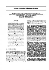
An E − m phase diagram showing the homogeneous (H) and inhomogeneous (I) phases and the coexistence curve. . . . . . . . . . . . . . . . . . . . . . .

34

3.2

Typical intermediate configuration for φ. . . . . . . . . . . . . . . . . . . . .

36

3.3

Typical intermediate configuration for φ. . . . . . . . . . . . . . . . . . . . .

37

3.4

Plot of q(t) vs. t showing transient behavior. . . . . . . . . . . . . . . . . . .

38

3.1

vi

List of Tables 3.1

Points on the coexistence curve shown in Figure 3.1. . . . . . . . . . . . . . .

35

3.2

Execution times for the different code segments. Tabulated values are an average over several iterations. . . . . . . . . . . . . . . . . . . . . . . . . . .

40

3.3

Performance on a sample problem vs. fill-in level. . . . . . . . . . . . . . . .

42

3.4

Execution times reflecting performance enhancements.

42

4.1

Convergence of nonlinear Gauss-Seidel iteration as a function of ∆t for E = 40. 44

4.2

Convergence of nonlinear Gauss-Seidel iteration as a function of ∆t for E = 80. 45

vii

. . . . . . . . . . . .

Chapter 1 Introduction Dr. James Langer, Chairman of the DOE-NSF National Workshop on Advanced Scientific Computing, 30-31 July 1998, wrote: [8] “. . . scientific computation has reached the point where it is on a par with laboratory experiment and mathematical theory as a tool for research in science and engineering. The computer literally is providing a new window through which we can observe the natural world in exquisite detail.” Indeed, we now have the ability to solve many problems arising in the natural sciences that would have been deemed intractable only a few decades ago. It cannot be overstressed, however, that scientific computation is a research tool no different than any other experimental apparatus. The creator and user of the tool is ultimately held responsible both for its performance and the accuracy and validity of the results it produces. Langer continues: [8] “It is essential to recognize that numerical simulation enhances, and does not substitute for, experimental and theoretical research. Meaningful simulations are based on reliable experimental and theoretical inputs, and their outputs are useful only if validated in the laboratory or the manufacturing plant. The best scientific simulations lead to new theoretical understanding and to new experimental discoveries.” Traditionally, scientists are not formally trained in the computing sciences. On average, some knowledge of a single programming language (usually Fortran or C) is the extent of their formal computer training. Conversely, most computer scientists do not possess formal training in a specific natural science beyond a college level course or two. In a subsequent letter to Physics Today on the same subject, Langer writes: [9] 1

Michael L. Parks

Chapter 1. Introduction

2

“We need better algorithms for solving various kinds of problems with new computing architectures, and better techniques for visualizing the data and extracting relevant information. We physicists will have to join forces with the mathematicians and computer scientists in developing these tools, and more of us will have to become computing specialists.” It is in this interdisciplinary frame of mind that this thesis covers the development and computational solution of an analytically intractible problem taken from nonequilibrium statistical mechanics. The remainder of this chapter covers the description of the driven lattice gas model with two species. The results of previous discrete simulations are discussed, and a continuum model of this system is developed. Chapter 2 describes an efficient numerical algorithm to determine a part of the phase diagram associated with this model. Performance enhancements to the algorithm are discussed. Chapter 3 presents the data collected. Chapter 4 discusses a convergence criterion that was discovered, and Chapter 5 summarizes the results, giving direction for future work. Appendix A contains the ELLPACK code that was used to generate the collected data.

1.1

Nonequilibrium Statistical Mechanics

Statistical mechanics is a branch of physics and chemistry that applies the methods of statistics to mechanical systems. It is the science of the phenomena of heat, or thermodynamics. Fundamentally, we contend that the macroscopic properties of matter should be explainable in terms of the motion of its parts. As such, statistical mechanics is the theoretical bridge between the microscopic world and the macroscopic world. In macroscopic systems, there may be 1023 microscopic particles, all of which are jumping about and interacting in a complex and seemingly random manner. In theory, we could use a very powerful computer to model the motions and interactions of all 1023 particles, but there is an easier and simpler way to draw conclusions about this system. If we assume the system to be isolated, we then believe it will eventually reach a time-independent equilibrium state, in which all of the particles are behaving in nearly the same manner. By applying statistical principles, we can then draw some conclusions about the properties of the macroscopic system [2]. This is possible because equilibrium properties are entirely dominated by statistics rather than by detailed dynamical mechanisms [3]. The study of equilibrium statistical mechanics has been very successful in explaining many phenomena. Although things like perfect insulators or infinite times are assumed, by approximating “perfect” insulators with “good” insulators and “infinite” time with “long” times, we can achieve measurable success in the real world because we have then approximated an equilibrium system. While physicists have had notable success in analyzing equilibrium systems, their study of nonequilibrium systems is not as well developed. Although this may be disappointing, it is

Michael L. Parks


3

certainly understandable. Equilibrium states consist mostly of dull uniform phases, while more interesting things like snowflakes, trees, and even graduate students are examples of physical systems in nonequilibrium steady (time-independent) states. Certainly, nonequilibrium systems are significantly more complex than their equilibrium counterparts. Thermal equilibrium cannot exist if the forces acting on a system are nonconservative, and so the traditional methods of analysis developed for equilibrium statistical mechanics are not applicable. In fact, all systems in nature are, in principle, nonequilibrium systems. It would be desirable to simply construct a new theory to deal with nonequilibrium systems, but this is a prohibitively formidable task. Worse, even the intuition developed while studying equilibrium systems is frequently not useful when applied to systems far from equilibrium. From the perspective of equilibrium phenomena, the behavior of nonequilibrium systems, even when in time-independent states, is frequently surprising [23]. To understand complex physical phenomena, physicists often construct simple models which are designed to capture the essence of the real world. In this spirit, some in-roads into the vast unknown of nonequilibrium statistical mechanics have been made through the study of simple models. In this endeavor, typically systems whose equilibrium behavior is reasonably well understood are chosen, so that the effects of nonconservative forces that drive the system out of equilibrium are readily apparent. While a simple model does not have enough complexity to approximate the real world, exploring the model may lead to a more complete understanding of the underlying phenomena involved. Such is the case with the driven two species lattice gas model considered here.

1.2

The Driven Lattice Gas Model with Two Species

An Ising lattice gas [4] consists of a rectangular lattice with each site empty or occupied by a single particle. The dynamics consists of particles “hopping” randomly to nearest neighbor sites, subjected to rates consistent with particles interacting via nearest neighbor attraction. In thermal equilibrium, this model is well-understood [11]. However, if a bias is applied in one direction [6], effectively a uniform DC “electric” field, the model is driven into nonequilibrium steady states and exhibits remarkably different and more complex behavior than the equilibrium Ising model. Many unexpected properties have been discovered for the driven Ising model [26, 19]. Most existing work has focused on this driven one-species model. However, Schmittmann and Zia have considered a generalization of this model containing not one but two species, having opposite charges [1, 21]. This two species model is developed below. Consider a square lattice, periodic in both directions, in which each site is either empty or occupied by a particle of either positive or negative “charge”. There may be at most one particle per lattice site. All particles have the same magnitude charge, and differ only in the sign. For simplicity, the total charge of the system is set to zero. That is, there are exactly

Michael L. Parks


4

as many positively charged particles in the system as negatively charged particles. The particles are allowed to hop randomly to nearest neighbor empty sites. The particles do not interact, except that one particle may not move to a site that is already occupied. Without any bias, such a system will evolve into a state where the particles are randomly distributed throughout the lattice. Such a state is an equilibrium state. To create a nonequilibrium state, the particle hops are biased through the application of an external “electric” field acting along the +y direction. Both particle number (mass) and total charge are held constant. Physically, this model system is similar to mapping the lattice onto the surface of a cylinder and applying a linearly increasing magnetic field down the main axis of the cylinder. The changing magnetic field will induce a constant electric field coiled around the main axis of the cylinder, which then serves as the drive. Note that any time independent states formed by this system are clearly nonequilibrium states, with non-zero “charge” currents. While this model system is primarily of theoretical interest, we note that it does have elements in common with real physical systems. For example, some ionic conductors, such as Ag2 HgI4 , have been observed to have two different ion species acting as charge carriers [23]. The system described above certainly yields itself to Monte Carlo simulation. There are two free parameters: E, the field strength in the +y direction, and the total number of particles. The total particle count is represented in m, the normalized average mass density of the system, and thus takes on values between 0 and 1. For the case E = 0, the distinction between the two charges becomes unimportant, and the particles hop randomly to nearest neighbor sites independent of charge. The E > 0 case introduces an asymmetry, where the particles now prefer to hop along or against the direction of the field, depending on the sign of their charge. A complete description of the details of the Monte Carlo simulation is done by Schmittmann, Hwang, and Zia [21]. We are considering the excluded-volume constraint, which means we are looking only at the high-field and high-temperature region. That is, we are not allowing any particle-particle interactions except that one particle may not move to a site that is already occupied by another particle. Simultaneous exchange of locations by two particles is not allowed in this model. This is a simple model, but a necessary first step towards the study of systems with more complex interactions [20].

1.2.1

Results and Discoveries from Previous Monte Carlo Simulations

A Monte Carlo simulation on the model system described above will frequently produce localized areas of high particle density that have become known as “clouds.” The naming is deliberately suggestive, as shown in Figure 1.1. The black particles carry a positive charge, the white particles carry a negative charge, and the holes have been colored blue. The field points in the +y direction. Free movement of the particles through the lattice is partially

Michael L. Parks


5

Figure 1.1: Typical “cloud” structure. blocked by the formation of these structures. While the behavior of the clouds is interesting in and of itself, the clouds do not represent a final time-independent state of the system. Monte Carlo simulations for longer times resulted in the discovery of an interesting phase transition. The clouds either dissipate completely, or merge into a single structure. When m < mc , where mc (E) is a field-dependent particle threshold density, all particles eventually distribute evenly over the grid, as shown in Figure 1.2. We refer to this state as the disordered or homogeneous phase. As the particle density is increased past mc , the particles segregate, forming a kind of “particle logjam” with a characteristic structure, as illustrated in Figure 1.3. We refer to this state as the ordered or inhomogeneous phase. We see that the excluded-volume interaction is, in fact, critical to the formation of this ordered state. The critical density was determined through Monte Carlo simulation by Schmittmann, et al., and is shown in Figure 1.4 [20]. It is useful to conceptualize mc (E) in the following way. If we decrease the field strength E, the particles return to hopping about randomly, and we expect the collection of particles to distribute themselves evenly over the lattice, thus ending up in a disordered state. If we decrease the total number of particles sufficiently, the particle density of the system is too low for a “logjam” to ever form, even for a strong field. If the lattice is dense with particles, even a moderate field will be sufficient to drive the particles into each other, forming the ordered state. Correspondingly, a strong field will also bring about an ordered state for a sufficiently high particle density, because movement will be dominated by jumps along or against the direction of the field. It was also found that the spatial structure of the inhomogeneous phase need not line up with the coordinate axis of the lattice, as shown in Figure 1.5 [1]. Consider a nonsquare lattice that is much larger in the x direction than the y direction. When simulated at m > mc ,

Michael L. Parks


Figure 1.2: Typical homogeneous configuration.

Figure 1.3: Typical inhomogeneous configuration.

6

Michael L. Parks


7

Figure 1.4: Typical critical density as a function of E for various system sizes [20].

Figure 1.5: Typical “barber pole” configuration. some resulting inhomogeneous states were found to be slanted with respect to the coordinate axis of the lattice. Given that the lattice being studied is periodic in both directions, these new inhomogeneous states quickly became known as “barber poles.” The “barber pole” configuration has been observed to be very stable.

1.3

Development of Continuum Model

While a Monte Carlo simulation of the system described above gives us some insight into its behavior, the goal of statistical mechanics is to understand the large-scale and long-time properties which are hopefully independent of the microscopic details of the model. The standard approach to this goal is to formulate a continuum model. In other words, we seek a set of “coarse-grained” equations of motion that capture the long-time and long-wavelength properties of the original lattice-gas. Such a model is developed in [21] and is summarized below. We begin by defining the spatial density of the positively and negatively charged particles

Michael L. Parks


8

as ρ+ (r, t) and ρ− (r, t), respectively. Since the densities of the particles are both conserved separately, they must separately satisfy the continuity equation: + ρ+ t +∇·j = 0 − ρ− t +∇·j = 0

(1.1)

where j ± represents the positive or negative current density, respectively. For a model such as this one, we suppose that the current is composed of two parts [22]. There will be a diffusive part that corresponds to the charged particle’s jumping randomly from one site to another, and a systematic part that corresponds to the charged particle’s desire to move along or against the applied field, according to the sign of its charge. We then suppose that the current density takes the form ± ± E yˆ) j ± = λ± (−∇µ

(1.2)

where λ± is a transport coefficient, µ± is the chemical potential, E is the coarse grained electric field (not to be confused with the microscopic electric field E), and yˆ is a unit vector in the +y direction, which is the direction of the field. We expect that λ± and µ± are both functions of ρ± . It is sufficient to assume that [22] µ± =

δH δρ±

(1.3)

where H is the Hamiltonian. We then have the current density as δH ± E yˆ). j± = λ± (−∇ δρ±

(1.4)

The equations that will result later take a much simpler form if ρ+ , ρ− are recast as φ(r, t) = 1 − (ρ+ (r, t) + ρ− (r, t)) ψ(r, t) = ρ+ (r, t) − ρ− (r, t)

(1.5)

where we see that φ has become the hole density and ψ has become the charge density. Taking the time derivatives of φ and ψ gives φt (r, t) = −ρ+ r, t) − ρ− r , t) t ( t ( · j − · j + + ∇ = ∇ · (j + + j − ) = ∇ r, t) − ρ− r , t) ψt (r, t) = ρ+ t ( t ( − · j − ∇ · j + = ∇ · (j − − j + ) = ∇

Michael L. Parks


9

Now, let us determine the forms taken by j + and j − . The Hamiltonian, in the absence of interactions, is purely entropic, and can be written as H = −S where S is the entropy of the system, which is the natural log of the multiplicity M associated with distributing N + and N − particles over a lattice of N sites. From combinatorics, we know that

M=

N N+

N − N+ N−

.

So,

S = = ∼ = =

N! (N − N + )! ln(M) = ln · (N − N + )!N + ! (N − N + − N − )!N − ! ln N! − ln N + ! − ln[(N − N + − N − )!] − ln N − ! [N ln N − N] − [N + ln N + − N + ] −[(N − N + − N − ) ln(N − N + − N − ) − (N − N + − N − )] − [N − ln N − − N − ] N ln N − N + ln N + − N − ln N − − (N − N + − N − ) ln(N − N + − N − )

where Stirling’s approximation is safely used since N, N + , and N − are in general large numbers. We can replace N + with Nρ+ , and N − with Nρ− , and, after some simplification, arrive at = −N(ρ+ ln ρ+ + ρ− ln ρ− + φ ln φ). (1.6) N is effectively a volume factor, so the Hamiltonian H is then H = ρ+ ln ρ+ + ρ− ln ρ− + φ ln φ.

(1.7)

Now that we have determined H, let us compute its functional derivatives with respect to ρ+ and ρ+ . δH δ = (ρ+ ln ρ+ − ρ− ln ρ− − φ ln φ) + δρ δρ+ = ln ρ+ − ln φ Similarly, δH = ln ρ− − ln φ. − δρ Recall that the transport coefficients λ± are dependent on ρ± . In general, we expect there to be no particle movement if there are no holes for a particle to jump to, or if there are simply no particles in the system. As such, we may set λ± = ρ± φ to within a constant, so that λ± now vanishes with ρ± and with φ. We now know enough to explicitly compute j + + j − and j − − j + so that we may describe the system completely in

Michael L. Parks


10

terms of φ, ψ, and associated constants:

+

−

j +j

= λ

+

δH + E yˆ + λ− −∇ δH − E yˆ −∇ + δρ δρ−

+ φψE yˆ = ∇φ

−

+

j −j

δH − E yˆ − λ+ −∇ δH + E yˆ = λ −∇ − δρ δρ+ − ψ ∇φ + Eφ(1 − φ)ˆ = φ∇ψ y. −

Plugging in, we can now complete the differential equations: · {∇φ + Eφψˆ y} φ t = Γ∇ · {φ∇ψ − ψ ∇φ − Eφ(1 − φ)ˆ y} ψt = Γ∇

(1.8) (1.9)

where Γ absorbs all other problem-dependent constants. Note that these equations must be augmented by specifying the boundary conditions to be periodic, and specifying conservation constraints on the total mass and charge:

φ dV

= (1 − m)V

(1.10)

ψ dV

= 0

(1.11)

where V is the volume of the system. In all subsequent references to equations 1.8 and 1.9, V is replaced with A because this thesis considers only the two-dimensional case. The description of the continuum model is now complete.

Chapter 2 Determining the Coexistence Curve The continuum model just described allows the theoretical prediction of some properties of the system that were observed with the Monte Carlo studies. In particular, two type of time-independent solutions were shown to exist [25], corresponding to the disordered, homgeneous state and the ordered, inhomogeneous state. Further, depending on the control parameters, these solutions are found to be stable against small perturbations. However, in some regions of the E − m phase diagram, both solutions are (linearly) stable. On the other hand, simulations show that typically only one of these is truly stable while the other is metastable. Only at the co-existence curve (a line in the E − m plane) can both states exist. We may draw analogy to the phase diagram for H2 O, shown in Figure 2.1. The lines defining the phase boundaries tell us at which pressures and temperatures two phases may coexist. The dot in the diagram indicates the “triple point” of water, which is the particular choice of pressure and temperature that allows the coexistence of all three phases. For a given pressure and temperature not on a boundary, the phase diagram tells us the state of the substance. Similarly, the coexistence curve in an E − m phase diagram delineates where the homogeneous and inhomogeneous phases may coexist in a time-independent state. However, unlike the case for H2 O, the system we are considering is not in equilibrium, for which no free energy exists. Thus, there is no analogous criterion by which a coexistence curve could be determined. Although the continuum equations, when endowed with proper noise terms, are believed to contain predictions for the coexistence curve, there are no simple analytic tools to unearth this result. Thus, we turn to numerical methods. To check these methods, we first reproduce the solutions of equations 1.8 and 1.9 in the unambiguously single phase regions. Then we define a criterion for “coexistence” and develop an algorithm to determine this curve.

11

Michael L. Parks

Chapter 2. Determining the Coexistence Curve

12

Figure 2.1: Phase diagram for H2 O.

Figure 2.2: An E − m phase diagram showing the homogeneous (H) and inhomogeneous (I) phases [25]. In the H + I region, one phase is stable and the other metastable.

Michael L. Parks

2.1


13

Algorithm Development

Considering the existing phase diagram shown in Figure 2.2 [25], we see that there are three main regions of interest. We label them H, I, and H + I. The curves defining the regions are theoretical stability limits developed by Vilfan, Zia, and Schmittmann in [25]. In the I region, only the inhomogeneous phase is stable. That is, all initial configurations of the system, given sufficient time, will converge to the inhomogeneous state. Similarly, in the H region, only the homogeneous phase is stable. Note that, for m greater than about 0.6282, the transition from one state to the other has already been determined analytically [25]. Since its nature is continuous, the amplitudes of the inhomogeneities develop continuously and there is no coexistence phenomenon. We will verify this line through numerical experiment. The coexistence curve itself is contained somewhere within the H + I region. In the H + I region but above the undetermined coexistence curve, the inhomogeneous phase is stable and the homogeneous phase is metastable. Similarly, in the H + I region but below the undetermined coexistence curve, the homogeneous phase is stable and the inhomogeneous phase is metastable. Classically, a system is said to be metastable if it is above its minimum-energy state, but requires an energy input before it can reach a lower-energy state. A metastable system can act like a stable system, provided that perturbations to the system remain below some threshold. A sufficient perturbation will “kick” a system from a metastable state into a stable state. The same “kick,” applied to a system in the stable state, will result in the system returning to the stable state. We may by analogy draw a “potential” diagram, shown in Figure 2.3, that represents the metastable and stable states. For our system, the deeper basin corresponds to the ordered configuration and the other basin to the disordered configuration, if we are considering an (E, m) above the coexistence curve. The exact opposite is true for an (E, m) below the curve. If the above picture was more than just an analogy, then coexistence can be defined as that set of control parameters which make the basin depths equal. However, due to the fact that our system is in a nonequilibrium steady state, such a “potential” is missing. Instead, we must define a “dynamic” criterion for coexistence and develop an algorithm to locate points on the coexistence curve in the H + I region. The notion of coexistence is based on the simultaneous presence of both phases in a system. By contrast, for a typical point in the H + I region of Figure 2.2, the stable phase will eventually be the final configuration. Thus, if we start with an initial configuration for φ and ψ that reflects a state close to being “half-ordered,” we can locate the coexistence curve by determining that set of (E, m) for which neither phase dominate at large times. To be specific, the “half-ordered” initial state consists of half of the system being the time independent disordered configuration and the other half being the time independent ordered configuration. Contour plots of φ and ψ for the inhomogeneous state are shown in Figures 2.4 and 2.5. The corresponding half-ordered configurations are shown in Figures 2.6 and 2.7. For an (E,m) system not on the coexistence curve, the half-ordered configuration must always select the stable state as its final state. Referring back to Figure 2.3, we note that the halfordered configuration would lie exactly in the middle of the figure, and thus will always select

Michael L. Parks


14

Figure 2.3: A “potential” diagram showing both stable and metastable states. the “stable” basin. Since the inhomogeneous phase is stable above the coexistence curve and the homogeneous phase is stable below the coexistence curve, the specific mechanism we choose to determine the coexistence curve’s location is as follows. For a fixed value of m, and some upper and lower bounds for E, we start with the half-order configuration and binary search in E. (E,m) systems that settle into the homogeneous final state are below the curve, and (E,m) systems that settle into the inhomogeneous final state are above the curve. Given that the coexistence curve itself does not correspond to stable system configurations, small perturbations will send the system into the homogeneous or inhomogeneous states. It is for this reason that we likely cannot determine the exact location of the coexistence curve in floating point, although we can bound its location tightly. To select a point in the E − m phase space, we need some mechanism to adjust both E and m. E is explicit in the model equations and can be represented numerically by a single or double precision IEEE floating point number, but representing m is more difficult. The choice of the initial configurations for φ, ψ effectively determines m. Recalling the additional constraints on the system description mentioned in equations 1.10 and 1.11, we see that m is determined by φ dA. Thus, we must determine some initial configuration for φ whose integral has the property that we desire. The time independent homogeneous configuration is specified by choosing φ = 1 − m and ψ = 0 for the entire domain. The time independent inhomogeneous state have been worked out by Vilfan, Zia, and Schmittmann [25] where φ is completely specified and ψ is computed from ψ=

−1 ∂ φ. Eφ ∂y

Michael L. Parks


Figure 2.4: Typical inhomogeneous configuration for φ.

15

Michael L. Parks


Figure 2.5: Typical inhomogeneous configuration for ψ.

16

Michael L. Parks


Figure 2.6: Typical half-ordered configuration for φ.

17

Michael L. Parks


Figure 2.7: Typical half-ordered configuration for ψ.

18

Michael L. Parks


19

This relationship may be arrived at through the following argument. If we consider equation + Eφψˆ 1.8, we recall that the term in braces, ∇φ y, is the hole current. Since the total charge of the system is zero, we expect there to be the same number of charged particles drifting along the direction of the field as there are charged particles drifting against the direction of the field, meaning that the net hole current in a time-independent state is zero. Setting the hole current to zero and only considering the single y direction of hole movement, we arrive at the above relationship. Unfortunately, the formula developed in [25] for the inhomogeneous time independent solution is numerically ill-conditioned and therefore problematic to use. The exact formula for the inhomogeneous configuration chooses m by expressing it in terms of an independent variable p, so that m = m(p). However, even small changes in p produce very large changes in m(p), meaning choosing a desired mass for the inhomogeneous configuration is very difficult. We avoid this difficulty entirely and instead generate the inhomogeneous time independent state numerically. Since the inhomogeneous state is at least metastable in the H + I region, we set the initial configuration of φ and ψ to a close approximation of the inhomogeneous state, then evolve the system in time, where it quickly converges to the inhomogeneous state. In practice, the formula for the exact solution was used (sometimes with the wrong p) to generate an approximate inhomogeneous configuration, which was then evolved in time until it converged to the correct inhomogeneous configuration. To generate the half-ordered configuration, we take the inhomogeneous configuration just computed and overwrite half of it with a homogeneous configuration. That is, half of φ is set to 1 − m, and half of ψ is set to zero. Since we numerically generate the inhomogeneous condition, we should try to reduce the time required for this step. For each (E,m) point we examine, we must generate an inhomogeneous state for that configuration. Since we are executing a binary search, the E values we consider are converging to some Ecritical , where (Ecritical , m) is a point on the coexistence curve. If we save the computed inhomogeneous state to disk, then reload it and use it as the initial condition for the next (E,m) system to be considered, we can greatly reduce the overall computation time for the construction of the half-order configuration, especially for later iterations in the binary search process. We now know how to generate a half-order configuration for any given (E,m) point in the phase diagram. Using this half-ordered configuration as an initial condition, we evolve the system in time, and watch to see if it converges to the homogeneous or inhomogeneous final state. Using that information, we select a new E and continue the binary search process until we have bound the location of the point (Ecritical , m) as tightly as desired. We may then repeat this process for many other values of m, until we have a sufficient number of points to approximate the coexistence curve. The process described above is illustrated in the psuedocode below.

Michael L. Parks 1 2 3 4 5 6 7 8 9 10 11 12 13 14 15 16 17 18


20

choose m choose Etop and Ebottom such that (Ecritical ,m) is contained within choose φ such that φ dA = 1 - m and φ inhomogeneous −1 ∂ φ choose ψ = Eφ ∂y write φ, ψ to disk while (Etop − Ebottom > tolerance) do 1 E = (Etop + Ebottom ) 2 restore φ, ψ from disk iterate (φ,ψ) until convergence to inhomogeneous state for (E,m) write φ, ψ to disk “chop” φ, ψ to generate half-order initial condition for current run while (system not converged to homogeneous or inhomogeneous states) do evolve system to next timestep od if (final state) == (inhomogeneous state) then Etop = E else Ebottom = E fi od

When determining points on the line of continuous transitions (i.e., m > 0.6282), the process is simpler than in the psuedocode above. For that domain, we may start with any ordered initial condition and evolve that system in time. If it converges to a homogeneous state, it is below the transition. If it converges to an inhomogeneous state, it is above the transition.

2.2

Algorithm Implementation

To determine the coexistence curve, we must be able to start with the half-ordered φ, ψ configuration for a particular choice of (E,m) and evolve those configurations in time according to the model equations 1.8 and 1.9. If we had only a single PDE to solve, we could simply employ a time-stepping method such as the Crank-Nicholson scheme, which is discussed in detail in Section 2.2.3. As we have a pair of coupled equations, we can employ the Crank-Nicholson method simultaneously for both equations, but we then need a mechanism for determining the solution for both equations at some fixed time. Thus, as an “inner loop” of the Crank-Nicholson scheme, we employ the nonlinear Gauss-Seidel method, which is discussed in detail in Section 2.2.4, to solve the pair of coupled equations at a fixed timestep. The nonlinear Gauss-Seidel method involves solving a sequence of large sparse linear systems arising from the discretized partial differential equations. The method of solution used here is GMRES, which is discussed

Michael L. Parks


21

in detail in Section 2.2.5. Finally, convergence criteria and an automated mechanism to determine the final state are discussed in Section 2.2.6. We choose to solve this system on the unit square [0,1]×[0,1] for times t=[0,T] where T is determined in relation to convergence criteria discussed later.

2.2.1

ELLPACK

Since the major portion of our work involves the solution of elliptic PDEs, the ELLPACK [13] system was used. ELLPACK is a well known Fortran 77-based software system for solving elliptic boundary value problems. It includes a very high level problem description language, and a library of problem solving modules. Fundamentally, ELLPACK will solve problems of the form Lu = auxx + 2buxy + cuyy + dux + euy + f u = g, where a, b, c, d, e, f and g are functions of x and y, but not of u or any of its derivatives, and Lu denotes the elliptic operator L applied to u. The ellipticity condition b2 − ac < 0 must hold for elliptic problems [13]. Boundary conditions may take the form p1 ux + p2 uy + qu = r where p1 , p2 , q, and r are again functions of x and y. Rectangular domains also admit periodic boundary conditions. After referring again to the model equations 1.8 and 1.9, we see that these are not in the form explicitly solvable by ELLPACK. Mathematically, the model equations take the form of a pair of coupled nonlinear time-dependent parabolic partial differential equations. Some cleverness is applied in subsequent sections to reformulate the model equations into a form solvable by ELLPACK.

2.2.2

Finite Difference Methods Overview

Finite difference methods attempt to compute a solution u(x, y, t) only at the points x = ı∆x, y = ∆y, t = +∆t, where ı = 0,1,2,. . . nx ,  = 0,1,2,. . . ny is called the “spatial grid” (or lattice, or net), + = 0,1,2,. . ., and where ∆t is assumed to be a small increment in time. As such, we are limited to determining the approximate solution only at the spatial points on the lattice, and only at the times that are integer multiple of the timestep ∆t. For this project, the following finite differences were used: ∂u u(x + ∆x, y, t) − u(x − ∆x, y, t) ≈ ∂x 2∆x 2 u(x + ∆x, y, t) − 2u(x, y, t) + u(x − ∆x, y, t) ∂ u ≈ 2 ∂x ∆x2

Michael L. Parks


22

and similarly for derivatives in the y direction. The discretization of the ut term is discussed in Section 2.2.3 in the context of the Crank-Nicholson method. These finite difference approximations all have a truncation error O(∆2 ). Like all finite difference methods, truncation error must be managed. Using these standard finite differences, our truncation error is O(∆x2 ) + O(∆y 2 ) + O(∆t2 ). (The truncation error for the ut discretization is also discussed in Section 2.2.3 with the Crank-Nicholson method.) Unfortunately, properties of the system that we would like to hold constant, such as the total charge or the total mass, are lost through the truncation error. Since we are computing our 1 solutions for the unit square, we have chosen to use a 200×200 grid, so ∆x = ∆y = 200 . Experimentally, the deviation of φ dA and ψ dA from desired values is minimal for even long times when this fine a mesh is used. Given the order of the truncation errors above, it is most reasonable to let ∆t = ∆x = ∆y so that the truncation errors are balanced. However, for stability reasons that arise from use of the nonlinear Gauss-Seidel method (see Chapter 4), the time increment ∆t is set to ∆x/10 = 0.0005. All data reported in later sections was collected using this spatial grid and timestep unless otherwise indicated.

2.2.3

Crank-Nicholson

The Crank-Nicholson method is a finite-difference method for solving time dependent PDEs. Crank-Nicholson was chosen over other common methods of solution because it is unconditionally stable for all choices of grid spacings ∆x, ∆y, and timesteps ∆t [14]. If we want to solve the problem ut = Lu + g(x, y, t) where L is an elliptic operator, then the Crank Nicholson method constructs a finite difference approximation “centered” at u(x, y, t+ ∆t ). It uses a centered difference in time to discretize the ut term. However, having no 2 ) + g(x, y, t+ ∆t ), it averages Lu(x, y, t+ ∆t) + g(x, y, t+ ∆t) information about Lu(x, y, t+ ∆t 2 2 and Lu(x, y, t) + g(x, y, t) to form an approximation: Lu(x, y, t + ∆t) + g(x, y, t + ∆t) + Lu(x, y, t) + g(x, y, t) u(x, y, t + ∆t) − u(x, y, t) = . ∆t 2 Note that the central difference in time with respect to u(x, y, t + ∆t ) now takes the form 2 of a forward difference in time centered at u(x, y, t), but still has a truncation error on the order of O(∆t2 ). Since we know u(x, y, t) and we want to solve for u(x, y, t + ∆t), we may rewrite this as Lu(x, y, t + ∆t) −

2 ∆t

2 u(x, y, t + ∆t) = − ∆t u(x, y, t) − Lu(x, y, t) −g(x, y, t + ∆t) − g(x, y, t)

(2.1)

where all the terms on the right hand side are known explicitly. Now, we may generate a linear system of equations and solve them to determine u(x, y, t + ∆t). By repeating this process, we iteratively step forward in time to compute the problem solution for future times.

Michael L. Parks


23

If we express equations 1.8 and 1.9 compactly as φt = Lφ φ + gφ (x, y, t), ψt = Lψ ψ + gψ (x, y, t), we can rewrite them in the form of equation 2.1. Lφ φ(x, y, t + ∆t) − Lψ ψ(x, y, t + ∆t) −

2 φ(x, y, t ∆t

2 ψ(x, y, t ∆t

2 + ∆t) = − ∆t φ(x, y, t) − Lφ φ(x, y, t) −gφ (x, y, t + ∆t) − gφ (x, y, t)

(2.2)

2 + ∆t) = − ∆t ψ(x, y, t) − Lψ ψ(x, y, t) −gψ (x, y, t + ∆t) − gψ (x, y, t)

(2.3)

One immediate problem is that ELLPACK does not provide a built-in mechanism for solving time dependent problems. By writing out the time dependency explicitly, we may reformulate the problem into one that ELLPACK can solve. This is shown in more detail in Section 2.2.7. Another difficulty in using the Crank-Nicholson method is that we have not one, but two coupled equations of the form above. In other words, Lφ and gφ depend on ψ, and Lψ and gψ depend on φ. While we can rewrite each equation in the Crank-Nicholson form (2.1), we must solve both equations 2.2 and 2.3 at each timestep before proceeding to the next timestep. The mechanism used to accomplish this is described in the next section.

2.2.4

Nonlinear Gauss-Seidel

Considering equations 1.8 and 1.9, one quickly notices that they are both nonlinear only when coupled with the other equation. As such, they are not “strongly” nonlinear, but in fact quasilinear. If we assume some initial guess for ψ and consider only equation 2.2 we see it takes the form of a linear elliptic PDE which we can solve using finite differences. If we solve for φ, we can then assume this solution is correct and move to equation 2.3. By the same analogy, we can solve that equation for ψ assuming φ is known, and then repeat this process, moving back and forth between the two equations. This process is reminiscent of the standard Gauss-Seidel iterative method, and is known formally as the “block nonlinear Gauss-Seidel method.” We iterate back and forth between the two equations until the φ, ψ solutions we generate stop changing from one iterate to the next, at which point we decide the system is converged, and that we have found the solution to the two coupled equations for some fixed time. We can now step the system forward in time according to the Crank-Nicholson scheme described above, and then repeat. This process is described in the psudeoscode below: 1 2 3 4

while (not(done)) choose φ choose ψ while φ, ψ not converged do

Michael L. Parks


24

Figure 2.8: Matrix pattern from systems with 2D periodic boundary conditions.

5 6 7 8

2.2.5

solve eqn. 2.2 using last computed value of ψ solve eqn. 2.3 using last computed value of φ od t = t + ∆t

Generalized Minimum Residual Method (GMRES)

The innermost step, the linear system solve, has yet to be discussed. Replacing the partial derivatives in equations 2.2 and 2.3 with finite differences results in large sparse systems of algebraic equations. We choose to use the linear solver GMRES [16]. The matrices associated with the linear systems we are solving have no special properties, other than that they are very sparse. Hence, an iterative method such as GMRES, which does not require special properties such as symmetry or definiteness, is appropriate. The linear systems we are solving take the general form shown in Figure 2.8. Note both the high level of sparsity and the characteristic band structure due to the finite difference stencil and the periodic boundary conditions enforced in both the x and y directions. For our 200×200 grid, the matrices themselves are nearly of dimension 4 · 105 × 4 · 105 . Because the bandwidth of the matrices is so large, performing band-Gauss elimination would be nearly as costly as ordinary (dense) Gauss elimination. The clear choice is to avoid direct methods altogether and focus on iterative methods that will take advantage of the sparsity of the matrix, and hopefully get the time for solution down well below the O( 23 n3 ) required of ordinary Gauss elimination [17].

Michael L. Parks


25

The idea behind GMRES is very simple. Suppose some x0 is our initial guess for the solution of the linear system Ax = b, with r0 = b − Ax0 the initial residual vector. Let W = Kl , where Kl is the lth Krylov subspace. That is, Kl = span{r0 , Ar, A2 r0 , . . . , Al−1 r0 }. At the lth iteration, GMRES forms an approximate solution xl ∈ Kl that minimizes the 2-norm of the residual vector rl = b − Axl . That is, given the linear system Ax = b, GMRES solves the problem min Ax − b 2 . x∈W Clearly, unless the true solution x is in Kl , then the residual vector will be nonzero. GMRES iterates by increasing the dimension of the Krylov subspace Kl → Kl+1 each iteration, hoping to reduce the residual further. In practice, to limit the total memory and computational requirements of GMRES, the integer η is defined as the “restart parameter”. If the dimension of the Krylov subspace reaches η without reducing the residual sufficiently, the entire GMRES process is restarted, with the initial x0 defined as xη from the previous GMRES iteration. The convergence criterion used for our implementation of GMRES is that rl 2 ≤ rtol· r0 2 +atol where r0 is the initial residual, rtol reflects the tolerance for a relative reduction of the residual, and atol represents a tolerance for an absolute magnitude of the residual. GMRES, like any iterative solution mechanism, requires an initial “guess” at the solution as a point at which to begin. This initial guess determines the initial residual. Effectively, our convergence criterion requires that the relative residual ≡ rl 2 / r0 2 be less than rtol, unless our initial guess was sufficiently good that atol is the dominant term, in which case we simply are requiring that rl 2 ≤ atol. The 2-norm of the residual vector is used here because it is generated “for free” as a byproduct of the GMRES process. Preconditioning GMRES A preconditioner modifies the coefficient matrix of a linear system of equations so that, in some sense, the linear system is easier to solve. Preconditioning the coefficient matrix before applying an iterative solution method may thus reduce the overall time to solution. Mathematically, to apply a preconditioner on the left, we transform the system Ax = b to

M −1 Ax = M −1 b

and effectively solve this transformed linear system. Effective preconditioners M −1 will approximate A−1 . In practice, the preconditioned matrix M −1 A is not formed explicitly.

Michael L. Parks


26

Instead, whenever the iterative solver calls for a matrix-vector multiplication (typically the dominant step for a Krylov solver) we first multiply by A and then solve a linear system involving M to compute the action of M −1 on the vector. Referring to the typical structure of the coefficient matrix for the linear systems we are solving as shown in Figure 2.8, we see that an ILU-type preconditioner would be effective. An ILU-type preconditioner involves the application of an incomplete LU factorization to the coefficient matrix, where L is lower triangular and U is upper triangular. If M = LU is an incomplete LU factorization of A, then the solution can proceed as described in the following psuedocode from [18, Algorithm 9.4]: 1 2 3 4 5 6 7 8 9 10 11 12 13 14 15 16 17 18 19 20 21

Compute r0 = M −1 (b − Ax0 ) Compute β = r0 2 Compute v1 = rβ0 for j = 1 to η do Compute w := M −1 Avj for i := 1 to j do hi,j :=< w, vi > w := w − hi,j vi od Compute hj+1,j = w 2 w Compute vj+1 = hj+1,j od Define Vη := [v1 , . . . , vη ] Define Hη = {hi,j }1≤i≤j+1; 1≤j≤η Compute yη = arg miny βe1 − Hη y 2 Compute xη = x0 + Vη yη if rj 2 > rtol· r0 2 +atol then x0 = xη GoTo 1 fi

When GMRES is preconditioned on the left, the Krylov subspace generated is not the one described previously, but is instead Kl = span{r0 , M −1 Ar0 , (M −1 A)2 r0 , . . . , (M −1 A)l−1 r0 } Necessarily, the computation of a complete LU factorization involves work proportional to O(n3 ) and is therefore too costly. Furthermore, the computed L and U matrices would in general be dense, and not reflect the same sparsity pattern found in the original coefficient matrix A. The creation of non-zero elements during Gaussian elimination is known as “fillin.” In addition to requiring our preconditioner to be easily computable, we do not want it to consume excessive storage. The ILU(p) preconditioner allows fill-in of p off-diagonals in computing both L and U. An additional difficulty with the ILU(p) type preconditioner is that it considers the structure of the matrix but does not consider the magnitude of the

Michael L. Parks


27

nonzero fill elements. The ILUT(p,τ ) preconditioner works as an ILU(p) preconditioner, but drops elements whose magnitude is less than τ (relative to the absolute value of the diagonal element) when computing L and U. The ILUT(p,τ ) preconditioner described above may fail for several reasons, all of which are effectively the same reasons that classical Gaussian elimination without pivoting may fail [18]. The implementation of the ILUT routine may underflow or overflow because of exponential growth of the entries of the factors L and U. The ILUT procedure may compute an incomplete LU factorization that is unstable. The ILUT procedure may encounter a zero pivot. Because the coefficient matrices we are operating with do not have a property that precludes zero pivots, such as positive definiteness, we cannot assume that a zero pivot will not be encountered. All of these problems may be remedied here, as well as in Gaussian elimination, through application of a pivoting strategy which is implemented in the ILUTP preconditioner, where the “P” stands for pivoting. A widely used implementation of several ILU-type preconditioners is found in SPARSKIT [15]. These preconditioners, as well as the GMRES solver in SPARSKIT were encorporated in ELLPACK and used for the numerical results reported in this thesis. Although not indicated by the diagram in Figure 2.8, the coefficient matrices are quite diagonally dominant. This can be made more visually apparent by considering the form of the discretization used in equation 2.1 to generate the coefficient matrices, and noting that ∆t < ∆x, ∆y to satisfy the stability condition arising from the use of the nonlinear Gauss-Seidel method. As such, it was experimentally found that allowing a fill-in of only 5 off-diagonals in the coefficient matrix is the best fill-in parameter for the problems studied here. Effectively, this means that an ILU-type preconditioner that allows a fill-in of only 5 off-diagonals in L and U effectively captures the “essence” of A−1 . A threshold τ of 1.0×10−3 was used as the drop tolerance. Again, given the strong diagonal dominance of the coefficient matrices, the use of smaller thresholds did not result in generation of a more cost-effective preconditioner. While the application of a cheaply-computed preconditioner may reduce the time for solution of a single linear system, the cost benefits increase greatly if a single preconditioner can be reused across many linear systems. We note in the nonlinear Gauss-Seidel process discussed in Section 2.2.4 that the inner loop iterates between solving two linear systems, neither of which change radically from one iteration to another. Thus, if we compute two preconditioners in the first iteration of the inner loop, one for each linear system, and reuse those preconditioners for the entire lifetime of the inner loop, the cost of solving the coupled system of equations will be reduced still further. Preconditioner reuse allows us to make a significant cut in the overall computational time to solution.

Michael L. Parks

2.2.6


28

Convergence Criteria

We also need an automated way to determine when the system has converged, as well as a mechanism to determine the final state of the system. One mechanism we can use involves watching the grid values of φ and ψ. We may decide that they have reached a time-independent state if their relative change from one iteration to the next is less than some threshold. When numerically constructing an inhomogeneous configuration before “chopping” it to construct a half-ordered configuration, this is the convergence criteria used. When we are interested in knowing the final state of a system without actually having to compute the final state explicitly, we need additional tools. Since φ and ψ are available for each gridpoint at each timestep, we may implement a “structure factor” in the spirit of the structure factor described by Schmittmann, Hwang, and Zia [21]. We define the structure factor as q≡

y

x

2

ψ(xi , yi )

where q is left unnormalized; q ≈ 0 when φ, ψ are in the homogeneous state, and q = qmax when φ, ψ are in the inhomogeneous state. Clearly, we may use this structure factor to determine the current state of the system. We may also use it to predict the final state of the system without actually computing it. Based on experimental evidence, after initial transients of q(t) die out, q(t) proceeds monotonically to either qmax or 0. Therefore, after waiting for some time t1 to allow any transient motion of q(t) to damp out, we may consider the sign of the slope of q(t) over several timesteps. If this value is unchanged, then q(t) is monotonic. Thus, we may conclude

final state =

Homogeneous for sign of slope of q(t) < 0, Inhomogeneous for sign of slope of q(t) > 0,

An example plot of q(t) is shown in Figure 2.9. For this particular choice of (E, m), the system converged to the inhomogeneous state. In some cases where E is far from Ecritical , the system nearly reaches its final state before time t1 . For these cases, “rails” have been implemented with the convergence criteria. That is, if q(t) grows too small or too large before time t1 is reached, the iteration terminates early with the decision that the final state will be ordered if q(t) is too large, and disordered if q(t) is too small. Since the inhomogeneous configuration defines qmax , q0 , the value of q(t) immediately after generation of the half-order initial condition, is 14 qmax . Fairly conservative “rails” have been set as qupper = 0.9qmax , and qlower = 0.05qmax . The rails are not symmetric in deference to the fact that q0 is not exactly between q = 0 and q = qmax . These rails are not used unless the system has nearly converged before time t1 , which only occurs when E is far from Ecritical .

Michael L. Parks


29

Figure 2.9: Typical plot of q(t) vs. t.

2.2.7

Problem Formulation for ELLPACK

In earlier sections, we noted that ELLPACK does not provide an explicit mechanism in software for solving time dependent problems or for solving systems of equations. We now discuss how these two goals may be accomplished in ELLPACK. First, we remove the time dependency from the problem by explicitly discretizing it using the Crank-Nicholson form, as was done in equation 2.1: u(x, y, t + ∆t) − u(x, y, t) = Lu(x, y, t + ∆t) + g(x, y, t + ∆t) + Lu(x, y, t) + g(x, y, t) ∆t If we manually insert code to increment t, we now have an equation in the form solvable by ELLPACK. The second difficulty is that ELLPACK was written to solve scalar equations of the form Lu = auxx +2buxy +cuyy +dux +euy +f u = g whereas we have the two coupled equations 2.2 and 2.3 to solve. We follow the template given by Rice and Boisvert [13] and allow ELLPACK to treat two equations by writing out the equation coefficients as Fortran-callable functions that switch on an equation index variable. That is, express the elliptic operator L acting upon u as Lu = a(x, y)uxx + 2b(x, y)uxy + c(x, y)uyy + d(x, y)ux + e(x, y)uy + f (x, y)u = g(x, y) where

a(x, y) =

uxx coefficient of first equation if keqn = 1, uxx coefficient of second equation if keqn = 2,

Michael L. Parks


b(x, y) =

30

uxy coefficient of first equation if keqn = 1, uxy coefficient of second equation if keqn = 2,

.. . where keqn is an equation index variable that is manually switched to cause ELLPACK to refer either to the first equation or to the second equation. The effect of the two elliptic operators Lφ and Lψ in equations 2.2 and 2.3 is now completely captured in the coefficients, leaving us with a single, “switched”, elliptic operator. In general, this scheme could be easily expanded to allow for many equations. The use of these two schemes makes ELLPACK capable of solving problems of the type we desire. We now proceed to formulate the two equations for use in ELLPACK, applying the schemes above. Rewiting equations 1.8 and 1.9 explicitly in two dimensions leaves φt = φxx + φyy + Eψφy + Eψy φ ψt = φψxx + φψyy − (φxx + φyy )ψ + Eφy (2φ − 1) We see that our general ELLPACK equation should take the form ut = a(x, y, t)uxx + b(x, y, t)uyy + e(x, y, t)uy + f (x, y, t)u + g(x, y, t) = Lu(x, y, t) + g(x, y, t) where

a(x, y, t) =

b(x, y, t) =

e(x, y, t) =

f (x, y, t) =

g(x, y, t) =

1 if keqn = 1, φ(x, y, t) if keqn = 2, 1 if keqn = 1, φ(x, y, t) if keqn = 2, Eψ(x, y, t) if keqn = 1, 0 if keqn = 2, Eψy (x, y, t) if keqn = 1, -(φxx (x, y, t) + φyy (x, y, t)) if keqn = 2, 0 if keqn = 1, Eφy (x, y, t)(2φ(x, y, t) − 1) if keqn = 2,

and L is our new switched elliptic operator. Rewriting equation 2.1 with our new switched elliptic operator L leaves Lu(x, y, t + ∆t) −

2 ∆t

2 u(x, y, t + ∆t) = − ∆t u(x, y, t) − Lu(x, y, t) − g(x, y, t + ∆t) − g(x, y, t)

and allows us to dispose of the two equations 2.2 and 2.3, having combined them into a single switched equation. This equation is now in a form solvable by ELLPACK.

Michael L. Parks

2.3


31

Overview of Software System

The psuedocode below illustrates the overall solution process. 1 2 3 4 5 6 7 8 9 10 11 12 13 14 15 16 17 18 19 20 21 22 23 24 25 26 27 28 29 30 31 32 33 34 35 36 37

choose m choose Etop and Ebottom such that (Ecritical ,m) is contained within E = 12 (Etop + Ebottom ) (* Generate initial φ,ψ configuration *) choose φ such that φ dA = 1 - m and φ an approximate inhomogeneous state −1 ∂ φ choose ψ = Eφ ∂y write φ, ψ to disk while (Etop − Ebottom > tolerance) do restore φ, ψ from disk (* Numerically generate the inhomogeneous configuration *) t=0 E = 12 (Etop + Ebottom ) while φ, ψ not in a time-independent state do while φ, ψ changed from last Gauss-Seidel iteration do solve eqn. 2.2 using last computed value of ψ solve eqn. 2.3 using last computed value of φ od t = t + ∆t od write φ, ψ to disk qmax = q(t) “chop” φ, ψ to generate half-order initial condition for current run t=0 (* Iterate system in time until convergence to homogeneous or inhomogeneous states *) while (NOT(converged)) do while φ, ψ changed from last Gauss-Seidel iteration do solve eqn. 2.2 using last computed value of ψ solve eqn. 2.3 using last computed value of φ od converged = ((t≥ t1 ) and (q(t) monotonic for last 20 timesteps)) or (q(t)≥ 0.9qmax ) or (q(t)≤ 0.05qmax ) t = t + ∆t od if ((q(t)too large) or (t > t1 and q(t) monotonic increasing for last 20 timesteps)) then Etop = E else Ebottom = E fi od

Michael L. Parks


32

Figure 2.10: Information flow between modules.

The actual binary search process is not implemented in ELLPACK, but in a separate program written in ANSI C. The program makes calls to ELLPACK, providing ELLPACK with an (E,m) point in the phase space, and ELLPACK returns with an identifier signifing the time independent state reached by the system. The information flow between processes is indicated in Figure 2.10.

2.4

Hardware

Data was collected on a 500 MhZ DEC Alpha running Digital UNIX V4.0E (Rev. 1091) using the ELLPACK May 1985 release. Some data was also collected on an Origin 2000 running IRIX Release 6.5 using the same ELLPACK release.

Chapter 3 Results and Observations The algorithm described above was executed for several values of m to numerically determine the location of the coexistence curve. Plots of the structure factor q(t) vs. t were also collected for all (E, m) systems considered, and examples are illustrated in subsequent sections. The inhomogeneous and homogeneous phases observed in the Monte Carlo simulations were reproduced through numerical solution of equations 1.8 and 1.9, keeping the constraints described in equations 1.10 and 1.11. A typical example of the inhomogeneous configuration is shown in the contour plots in Figures 2.4 and 2.5. The corresponding homogeneous configuration is not pictured, because the corresponding contour plot has no contours. Also, the general relationship between the drive and the critical mass density of the system depicted in Figure 1.4 was reproduced in Figure 3.1.

3.1

The Coexistence Curve

The complete phase plot is shown in Figure 3.1. A table of the data points collected is shown in Table 3.1. Since the points on the curve were found via a binary search process, the actual point Ecritical could be anywhere in the range (Etop , Ebottom ). We have tabulated Ecritical as the average of Etop and Ebottom . We start by noting that the location of the line of continuous transitions (i.e., m > 0.62) determined by our methods agrees with the theoretical prediction. The lack of data points between m = 0.450 and m ≈ 0.62 is due to the fact that the “curve-locating” algorithm discussed earlier requires an initial Etop and Ebottom in the H + I region of the phase diagram. As is apparent from Figure 3.1, picking an initial Ebottom in the H + I region of the phase diagram for m > 0.450 is difficult. If the initial Ebottom is in the H region of the phase diagram, the numeric generation of the inhomogeneous configuration used to create the “half-order” 33

Michael L. Parks

Chapter 3. Results and Observations

34

Figure 3.1: An E − m phase diagram showing the homogeneous (H) and inhomogeneous (I) phases and the coexistence curve.

configuration is not always guaranteed, and the algorithm may fail. Since the coexistence curve must intersect the lower boundary of the H + I region as m nears 0.62, the lack of experimental data for 0.450 < m < 0.700 in this region is not significant.

3.2

Typical System Configurations During Solution Process

Contour plots were collected from ELLPACK during various stages of the solution process illustrating typical system configurations. Figures 2.6 and 2.7 show the half-order configurations for φ and ψ, which are taken as the initial condition for the system for reasons described in Section 2.1. The system’s time evolution takes different paths at this point dependent on its final state. If the choice of (E, m) is such that the final state is inhomogeneous, we see the near vertical contour lines from the initial configuration “unfurl” as the system is evolved in time. Eventually, the system becomes homogeneous in the x direction and inhomogeneous in the y direction, the direction of the field. If the choice of (E, m) is such that the final state is homogeneous, we see the near vertical contour lines from the initial configuration “unfurl” as before, but the resulting system becomes homogeneous in both the x and y directions. These intermediate steps are illustrated in Figures 3.2 and 3.3 for φ and ψ, respectively. We note also that for many systems, the structure factor q(t) is not always monotonic. That is, it does not always proceed directly to its final state of 0 or qmax , but instead passes

Michael L. Parks


m ±0.0001 0.250 0.275 0.300 0.325 0.350 0.375 0.400 0.425 0.450 0.700 0.725 0.750 0.775 0.800 0.825 0.850 0.875 0.925 0.950 0.975

Etop

Ebottom

Ecritical

87.788 70.988 59.025 49.927 42.397 35.356 30.687 26.583 23.616 9.940 9.370 8.890 8.480 8.120 7.800 7.515 7.260 6.820 6.630 6.450

87.781 70.981 59.019 49.921 42.390 35.348 39.679 26.573 23.607 9.930 9.360 8.880 8.470 8.110 7.790 7.505 7.250 6.810 6.620 6.440

87.785 70.985 59.022 49.924 42.394 35.352 30.683 26.578 23.612 9.935 9.365 8.885 8.475 8.115 7.795 7.510 7.255 6.815 6.625 6.445

Table 3.1: Points on the coexistence curve shown in Figure 3.1.

35

Michael L. Parks


Figure 3.2: Typical intermediate configuration for φ.

36

Michael L. Parks


Figure 3.3: Typical intermediate configuration for φ.

37

Michael L. Parks


38

Figure 3.4: Plot of q(t) vs. t showing transient behavior.

through intermediate states that are either more ordered or more disordered than the initial state. A sample plot of some of the transient behavior is shown in Figure 3.4. All transient behavior is observed experimentally to damp out by the time t1 = 0.1, which supports the validity of the convergence criteria described in Section 2.2.6.

3.3

Motion Pictures : A System from Start to Finish

The attached .avi files show a motion picture of the contour plots of φ and ψ starting with the initial conditions (m, E) = (0.350, 45.0) and (m, E) = (0.350, 30.0), the first of which converges to an inhomogeneous state, and the second of which converges to a homogeneous state. The behavior of the systems depicted in these movies is characteristic of all of the systems examined.

3.4

Discussion of Error

Numerical error is capable of causing serious problems at several different stages of the solution process. First and foremost, the finite difference schemes we are using are not conservative of charge or mass, both of which should be system invariants. By decreasing

Michael L. Parks


39

the truncation error through use of a fine grid and small timestep, the values for φ dA and ψ dA were bound to vary less than ±0.0001. This was checked at each timestep through the use of the quadrature routine TWODQ, part of the package CMLIB available at http://gams.nist.gov. To ensure that the solutions computed were in fact valid, the point (Ecritical , 0.400) was also computed for a 400×400 grid with timestep 0.00025, and found to converge to the same solution (±0.02 in E) as on a 200×200 grid with the usual timestep 0.0005. In this sense, we feel that the solutions we have computed are in fact converging on the spatial grid used. Finally, we note an error that may occur when dealing with systems where (E, m) is very close to (Ecritical , m). Recall that m is not represented explicitly in the model equations 1.8 and 1.9, but is instead represented implicitly as 1 − φ dA. Numerically, it is represented in the table storing φ. Subtle changes in that table can cause m to fluctuate from iteration to iteration. As our binary search process converges on the point (Ecritical , m), the final state selected by the system becomes sensitively dependent on m. Because m is constantly changing from iteration to iteration (where again the total change is less than ±0.0001) the small fluctuations in m may “kick” our system from one state to another early in the solution process, thus resulting in the wrong final state being selected for the particular (E, m) system being considered. It is also this behavior that keeps us from being able to determine a point exactly on the coexistence curve in floating point. Fortunately, the spatial grid is fine enough that fluctuations in m are less than 0.0001. If this error occurred, the final location of the coexistence curve would be incorrect by at most 0.0001 in m.

3.5

Discussion of Time Requirements

The time to execute 200 timesteps (to advance t from 0.0 to 0.1) varies with the choice of E and m, with higher numerical values of E and lower numerical values of m requiring more computational time. The increased time cost is manifested in a larger number of Gauss-Seidel iterations per timestep. Experimentally, the choice of E influenced the overall computational time much more strongly than the choice of m. Given the material discussed in Chapter 4, this is reasonable. Since ∆t is kept fixed, a larger numerical value of E makes the coefficient matrices generated in the nonlinear Gauss-Seidel process less diagonally dominant. Presumably even larger values of E would eventually lead to nonconvergence of the nonlinear Gauss-Seidel process. For the DEC Alpha configuration described in Section 2.4, the highest time cost to compute 200 timesteps for some (E, m) in the H + I region was 5139 seconds, for (E, m) = (90, 0.25). The lowest time cost of 1851 seconds was observed for (E, m) = (30, 0.4). Of that time, most is spent on solving systems of linear equations. The overall time required for solution can typically not be predetermined for an iterative method. However, the mean time required for performing the individual steps in the solution process can be estimated.

Michael L. Parks


Code Segment Compute initial half-order condition Generate coefficient matrix Generate initial solution vector GMRES setup (preconditioner generated) GMRES setup (preconditioner reused) solve linear system with GMRES compute structure factor q perform quadrature with TWODQ()

40

Average Execution Time (seconds) Variable 0.29 0.05 0.32 0.03 0.22 0.0007 0.005

Table 3.2: Execution times for the different code segments. Tabulated values are an average over several iterations. The time requirements for each stage of the solution process are listed in Table 3.2. The times presented here are an average over 200 timesteps for (E, m) = (40, 0.4). There was a low variance between iterations, so the tabulated values are good approximation of the true mean values, except for the case of the linear solve. For initial nonlinear Gauss-Seidel iterations, GMRES typically took more iterations to converge than for later nonlinear Gauss-Seidel iterations. This should be expected, because in later nonlinear Gauss-Seidel iterations, φ and ψ are effectively converged, meaning that GMRES starts with a vary good initial guess, and can complete in only 2 or 3 iterations, which typically requires only 0.02 or 0.03 seconds. The generation of the initial half-order condition first requires the numerical computation of an inhomogeneous configuration, the cost of which is variable depending on how far the computation has proceeded with the binary search process, for reasons discussed in Section 2.1. Recall that preconditioners are reused for all linear solves except the first within a single timestep. As such, the cost for the “GMRES setup” is 0.03 seconds for most cases, and is 0.29 seconds only twice a timestep (once for φ, and once for ψ.) The overall time to bound a single (E, m) on the coexistence curve is an integer multiple of the time required to execute 200 timesteps, which is the time taken to determine if some (E, m) is above or below the coexistence curve. Since we bound points on the coexistence curve through a bisection search, the initial values of Etop and Ebottom control the number of subsequent (E, m) systems considered. Picking the initial Etop always no more than 100 and the initial Ebottom always large enough to be in the H + I region for a particular m, there are typically 13 or fewer bisections required to bound a point on the coexistence curve for a particular m.

Michael L. Parks

3.6


41

Discussion of Performance Enhancements

The average execution times presented in Section 3.5 reflect a code optimized to solve this particular problem. Initial versions of ELLPACK code took nearly four hours to process 200 timesteps on a 60 × 60 mesh, whereas our improved implementation requires at most 1.5 hours using a 200 × 200 mesh. Since the program spends most of its time generating and solving linear systems, the greatest benefit can be had by speeding up this process via any means possible. The first prototype code used band-Gauss elimination, a direct method, to solve the linear systems generated. The computational cost of band-Gauss elimination can be shown to be O(p2 m) where p is the bandwidth of the m × m matrix being operated upon. The periodic boundary conditions in both the x and the y directions along with the finite difference stencil cause the bandwidth to be nearly m, as shown in Figure 2.8. As our coefficient matrices are n2 × n2 , with an n × n mesh placed on the unit square, the cost of band-Gauss elimination becomes O(n6 ). This is coupled with the memory requirements being O(n4 ) due to fillin during the solution process. These prohibitive computational and storage costs lead to immediate rejection of direct methods in favor of iterative methods, which for the present problem require significantly less time. Furthermore, our storage costs are significantly reduced (to O(n2 )) because we only need to store the nonzero elements of the coefficient matrices plus the additional space required by ILUT. The iterative method selected, for reasons discussed in Section 2.2.5 was GMRES. Preconditioned GMRES was found to have significantly better performance than non-preconditioned GMRES. Table 3.4 shows that use of a preconditioner improved the performance of GMRES by over a factor of two. Also, preconditioned GMRES was found to converge in less than 30 iterations in almost all cases observed. Non-preconditioned GMRES, however, required a restart parameter over 100 to obtain convergence in many cases. The lower restart parameter allowed by preconditioned GMRES also reduces the total memory cost for the GMRES process. ILUTP preconditioning applied on the left was experimentally found to be the best preconditioner choice, resulting in faster overall execution of GMRES than ILUTP applied on the right, or ILU applied on either the left or right. A fill-in of 5 off-diagonals was also experimentally found to result in the overall fastest execution of the GMRES process, as shown in Table 3.3. This data reflects the system (E, m) = (58.772, 0.3) (close to Ecritical ) run for 10 timesteps. The number of GMRES iterations vary widely within a single timestep, becoming largest near the beginning of the timestep, and smallest near the end of the timestep when φ and ψ have effectively converged. Since the nonlinear Gauss-Seidel process involves solving nearly the same linear systems each iteration, we find that reusing preconditioners across successive Gauss-Seidel iterations further enhances performance. For the test case where 200 timesteps were computed for the system (E, m) = (40, 0.4) on a 200 × 200 mesh, preconditioner reuse dropped the overall execution time from 63.7 minutes to 54.1 minutes, while increasing the average number of

Michael L. Parks


42

Fill-In Level Max/Min GMRES Iterations Execution Time (seconds) 6 10/2 251.33 5 11/2 247.33 4 12/2 247.37 3 20/3 286.57 Table 3.3: Performance on a sample problem vs. fill-in level. Code Segment “Vanilla” GMRES Preconditioned GMRES + Preconditioner reuse + Function and derivative caching

Average Execution Time (minutes) 160.7 63.7 54.1 39.3

Table 3.4: Execution times reflecting performance enhancements. GMRES iterations from 6.28 to 6.35. Some increase is expected, because (in general) a slightly worse preconditioner is being used each iteration. The idea of preconditioner reuse is validated in that the total time cost was reduced, and the average number of GMRES iterations did not increase drastically. This means that the reused preconditioner wellapproximates the action of a preconditioner generated explicitly for each linear system to be solved. A final optimization involves improving the efficiency of the discretization process. A straightforward implementation of our algorithm using ELLPACK results in a very inefficient matrix generation step. In particular, in building the linear systems, ELLPACK must evaluate the PDE coefficients and “right hand side” function at each of the grid points. For our problem, many of these functions depend on recently computed values of φ or ψ or one of their derivatives. The needed values are determined with biquadratic interpolation out of tables of stored values. Considerable redundant work can be avoided if this interpolation is done only once per grid point, and for all needed derivatives of φ or ψ, rather than each time a single function value or derivative is needed. Since ELLPACK does not assume there is any particular relationship among the PDE coefficients, it cannot take advantage of this optimization. By taking advantage of this observation however, we can save a significant amount of time in the discretization phase. The effects of the performance enhancements described above are summarized in Table 3.4, which shows the cost of computing 200 timesteps for the system (E, m) = (40, 0.4) on a 200 × 200 mesh. The cost of band-Gauss elimination is not tabulated, however, because performing band-Gauss elimination on a 200×200 mesh would require over 1000 hours of computing time and nearly five gigabytes of memory, which well exceeds the available memory on either of the machines discussed in Section 2.4.

Chapter 4 Convergence Criterion for the Nonlinear Gauss-Seidel Method We observe that not all choices of ∆x, ∆y, and ∆t result in convergence of the nonlinear Gauss-Seidel process. We choose ∆x and ∆y small enough to avoid undesirable fluctuations in the total mass and charge. It is common to let ∆t = ∆x = ∆y in the Crank-Nicholson method to balance the truncation error. However, with this choice of timestep, for large enough E, the nonlinear Gauss-Seidel process does not converge. Fortunately, this difficulty can be avoided by decreasing ∆t. This suggests that for a fixed grid spacing there is a convergence criterion controlled by the choice of ∆t and E. We must have the freedom to choose a large E in order to investigate the coexistence curve, meaning that ∆t must be reduced correspondingly. For a 200 × 200 mesh, ∆t = 0.0005 is small enough to allow convergence for all E investigated. The Crank-Nicholson method is unconditionally stable for all choices of ∆x, ∆y, and ∆t. However, application of the Crank-Nicholson method leads to the generation of linear systems which may not be solvable with an iterative method. For example, if we applied the CrankNicholson method to a single PDE, we would generate a single system of linear equations at each timestep that must be solved in order to proceed to the next timestep. We could then attempt to solve each linear system of equations using an iterative method such as the GaussSeidel method. It is an established convergence result for the Gauss-Seidel method that if the coefficient matrix is diagonally dominant, the Gauss-Seidel method will converge [18]. (The theorem does not go the other direction—if the coefficient matrix is not diagonally dominant, the Gauss-Seidel method may or may not converge.) Thus, if the coefficient matrix is not diagonally dominant we cannot be guaranteed that the Gauss-Seidel method will converge. To ensure convergence, we must then either adjust our mesh and timestep to make the generated coefficient matrix diagonally dominant, or choose another linear solver. For the problem at hand, we are not using the pointwise Gauss-Seidel method on linear systems, but instead a block nonlinear Gauss-Seidel method. The blocking is chosen, of course, to 43

Michael L. Parks Chapter 4. Convergence Criterion for the Nonlinear Gauss-Seidel Method 44 ∆t Strictly Diagonally Dominant 0.0005 Yes 0.0010 Yes 0.0015 Yes 0.0020 No 0.0030 No 0.0050 No

Convergent GS Iteration Yes Yes Yes No No No

Table 4.1: Convergence of nonlinear Gauss-Seidel iteration as a function of ∆t for E = 40. take advantage of the fact that equations 1.8 and 1.9 are quasilinear. Thus, our choice of blocks produces two sets of linear equations, instead of two sets of nonlinear equations, where it is given that solving linear equations is preferable to solving nonlinear equations. We solve the generated linear systems of equations with GMRES, which does not have convergence problems for large enough values of the restart parameter. Thus, the observed convergence criterion is due entirely to the use of the nonlinear Gauss-Seidel method. The choice of E as a problem parameter and ∆t as a timestep in the Crank-Nicholson method directly affect the structure of the generated coefficient matrices, and thus the convergence of the nonlinear Gauss-Seidel process. Unfortunately, we are not aware of any published theorems regarding the convergence of the block nonlinear Gauss-Seidel method. By making comparisons with the linear pointwise Gauss-Seidel method, we numerically investigate this convergence criterion. 1 Referring to equations 2.2 and 2.3, we see that a factor of ∆t is contained within the diagonal of the generated coefficient matrix, whereas E contributes to the magnitude of the off-diagonal elements of the coefficient matrix. Thus, larger values of E may result in CrankNicholson generating coefficient matrices that are not diagonally dominant. Systems with larger numerical values of E for timesteps ∆t too large were observed to have nonconvergent Gauss-Seidel iterations. Decreasing ∆t, as discussed above, resulted in a convergent GaussSeidel process and increased the diagonal dominance of the coefficient matrices. So, it is not unreasonable to assume that there is in fact a connection between the diagonal dominance of the coefficient matrices generated by the Crank-Nicholson process and the convergence of the nonlinear Gauss-Seidel method.

This hypothesis was investigated numerically in two experiments, both of which fixed ∆x = 1 ∆y = 200 , m = 0.4, and allowed ∆t to vary. The first experiment chose E = 40, and the second chose E = 80. The system was evolved in time until either 10 timesteps had been computed, or until the nonlinear Gauss-Seidel process failed to converge. All coefficient matrices were examined before each linear solve for strict diagonal dominance. The collected data is shown in Tables 4.1 and 4.2. Note that in Tables 4.1 and 4.2, the “strictly diagonally dominant” column is marked “yes” only if every matrix encountered in the first 10 timesteps is strictly diagonally dominant,

Michael L. Parks Chapter 4. Convergence Criterion for the Nonlinear Gauss-Seidel Method 45 ∆t Strictly Diagonally Dominant 0.0005 Yes 0.0010 Yes 0.0015 No

Convergent GS Iteration Yes Yes No

Table 4.2: Convergence of nonlinear Gauss-Seidel iteration as a function of ∆t for E = 80.

i.e., | aii |> i=j | aij | for a matrix A. Later timesteps were not investigated due to the high cost of this process. As such, this does not preclude the possibility that matrices generated later were not strictly diagonally dominant. Although there are no established convergence criteria for the nonlinear block Gauss-Seidel method, there is evidence supporting the idea that the corresponding (linear) blocks of equations, if diagonally dominant, can ensure convergence.

Chapter 5 Conclusions and Future Work 5.1

Results and Conclusions

In this thesis we describe a lattice gas with equal numbers of oppositely “charged” particles diffusing under the influence of a uniform “electric” field and the excluded volume condition. The results of previous discrete simulations are discussed. The discrete simulations predict the existence of two phases, one spatially homogeneous and one spatially inhomogeneous, controlled by the external field strength and particle density. Characteristic examples from the discrete simulations of the inhomogeneous and homogeneous phases are shown in Figures 1.3 and 1.2, respectively. Points on the coexistence curve for the discrete model for various system sizes are shown in Figure 1.4. A continuum model of this system was developed by Schmittmann, Hwang, and Zia [21], and exact solutions for the inhomogeneous time-independent state were determined [25]. In this thesis, an iterative solution technique employing the block nonlinear Gauss-Seidel method was implemented to numerically solve the equations 1.8 and 1.9 describing the continuum model with the constraints in equations 1.10 and 1.11. The constraints in equations 1.10 and 1.11 effectively enforce conservation of mass and charge. These conservation requirements are not enforced explicitly during the numerical solution process, but rather implicitly in the choice of spatial grid size, which was chosen fine enough to permit fluctuations in the total mass and charge of the system of less than ±0.0001. The block nonlinear Gauss-Seidel method exhibited a convergence criterion, which forced the choice of a timestep ∆t much smaller than the grid spacing ∆x and ∆y. The existence of time independent spatially inhomogeneous and spatially homogeneous phases predicted by the discrete model and also theoretically for the continuum model was observed numerically. A characteristic example of the inhomogeneous phase is shown in Figure 2.4. A characteristic example of the homogeneous phase is not depicted because it

46

Michael L. Parks

Chapter 5. Conclusions and Future Work

47

has no contour lines and is, by definition, uniform everywhere. A plot of the numerically determined coexistence curve for the continuum model is shown in Figure 3.1. The initial algorithm developed was optimized through the use of an ILU-type preconditioner whose parameters were tailored to the problem at hand. Performance was further enhanced by reusing that preconditioner for all linear solves through a single timestep. Performance was subsequently improved further by caching derivative and function values for φ(x, y) and ψ(x, y), which accelerates the generation of coefficient matrices used in the linear system solves. Overall, the time requirements were reduced by a factor of four over the straightforward method, allowing the continuum model equations to be solved much more efficiently. The software system developed is general enough to allow further investigation of related models without a significant rewrite. For example, systems where the total charge is nonzero, considered in the next section, can be solved on the existing software system. Further properties of this system, such as the stability limits separating the I, H + I, and H regions of Figure 3.1 could also be determined.

5.2

Future Work

The model examined is perhaps the simplest possible noninteracting two species model. The next logical step is to consider a model where neighboring oppositely charges particles are allowed to swap locations [7]. The corresponding continuum model is : · {∇φ + Eφψˆ φ t = Γ∇ y} (5.1) γ · {γ ∇ψ + (1 − γ)[φ∇ψ − ψ ∇φ] − Eφ(1 − φ)ˆ y − E[(1 − φ)2 − ψ 2 ]ˆ y } (5.2) ψt = Γ∇ 2 where γ is the probability of two oppositely charges particles swapping locations. We note, of course, that if we take γ = 0, the equations reduce to 1.8 and 1.9, the model equations investigated in this thesis. A further modification to this model is to assume the total charge is nonzero. That is, let ψ dA ≡ Q = 0, and investigate the behavior of the system. Brookings and Zia have collected data from discrete simulations to build up a complete phase diagram in (E-m-Q) space, although these results have not yet been published. Though the continuum equations are the same as those considered here, the inhomogeneous solutions are quite different. In particular, the spatial structure is predicted to drift with a constant velocity, a phenomenon observed in simulations [10]. On the computational side, it is possible to reuse preconditioners not only across a single timestep, but across multiple timesteps. This would only be a reasonable approach if the φ(x, y) and ψ(x, y) systems were not changing much from timestep to timestep. That is, preconditioner reuse across timesteps would make the most sense when the system is nearly

Michael L. Parks

Chapter 5. Conclusions and Future Work

48

converged, and will soon reach a time-independent state. Parallelism has been exploited so far only in the trivial case. That is, multiple points on the coexistence curve may be computed in parallel. On a nontrivial level, the matrix-vector multiply in GMRES will parallelize easily. However, the ILU factorization and application will not. There has been a recently proposed parallel version of ILU [5], however, that would allow the ILU factorization and application to occur in parallel. Domain decomposition methods would also allow for parallelization of this problem [24, 12].

Appendix A The ELLPACK Source Code * Ellpack program to solve time dependent system of 2 PDEs. * * Outer loop is over time (see Section 5.D of Rice & Boisvert). * Inner loop is over 2 eqns (see Section 5.E of Rice & Boisvert). * option. level = 0 * tcur = current simulation time * deltat = timestep * nstep = integer number of current timestep global. real tcur, deltat integer nstep common /gcomon/ tcur, deltat, nstep declarations. * * Set parameters: * * maxiter = max number of iterations for inner loop * thresh = threshold for convergence of inner loop, i.e., need * relative change in both phi and psi less than this. * parameter (maxiter=50, gsthresh=1.0e-11,timethresh=1.0e-3)

49

Michael L. Parks

Appendix A. The ELLPACK Source Code

50

* * Data structures to keep track of 2 equations and solutions * * keqn = keeps track of which eqn I’m on. * phitbl = holds most recent phi solution at current time * phioldtbl = holds phi solution at previous GS iteration * phioldtime = holds phi solution at previous timestep * psitbl = holds most recent psi solution at current time * psioldtbl = holds psi solution at previous GS iteration * psioldtime = holds psi solution at previous timestep * cache holds function and derivatives values, as well as ‘‘dirty bit’’ common /switch/ keqn common /savphi/ phitbl ($i1ngrx,$i1ngry),phicache(9) common /savgsphi/ oldgsphitbl ($i1ngrx,$i1ngry),oldgsphicache(9) common /savtimephi/ oldtimephitbl($i1ngrx,$i1ngry) common /savpsi/ psitbl ($i1ngrx,$i1ngry),psicache(9) common /savgspsi/ oldgspsitbl ($i1ngrx,$i1ngry),oldgspsicache(9) common /savtimepsi/ oldtimepsitbl($i1ngrx,$i1ngry) common /pparam/ epsilon * * Variable declarations for preconditioner storage & reuse * use three arrays to store a single preconditioner in CSR format * storage for phi preconditioner * real a1_save * integer ja1_save, ia1_save * storage for psi preconditioner * real a2_save * integer ja2_save, ia2_save real a1_save($lupreconmaxnz) integer ja1_save($lupreconmaxnz), ia1_save($i1mneq+1) real a2_save($lupreconmaxnz) integer ja2_save($lupreconmaxnz), ia2_save($i1mneq+1) * * Variable declarations for main loop * * * converged = has the physical system (outer iteration) converged yet? * GSconverged = has the gauss-seidel (inner iteration) converged yet? * nunks = number of unknowns

Michael L. Parks * * * * * * * * * * *


tstart = start time of simulation (usually 0.0) tstop = simulation end time GSdelphi = max change in phi table from last GS iteration GSdelpsi = max change in psi table from last GS iteration timedelphi = max change in phi table from last timestep timedelpsi = max change in psi table from last timestep qmax = the value of Q() in a near-inhomogeneous state qval = the most recently computed value of Q() qarr = the n most recently computed values of Q() mass = the mass of the system (not used in computation) finalstate = the final system state (H,I,O) logical converged logical gsconverged integer nunks real tstart real tstop real gsdelphi real gsdelpsi real timedelphi real timedelpsi real qmax,qval real qarr(1:20) real mass character finalstate

equation. cfuxx(x,y)*uxx + cfuyy(x,y)*uyy + cfuy(x,y)*uy & + (cfu(x,y)-2./deltat)*u = pders(x,y) boundary. periodic on on on on

x x y y

= = = =

0.0 1.0 0.0 1.0

grid. 200 x points 200 y points fortran. nunks tstart tstop deltat nsteps

= = = = =

i1ngrx*i1ngry 0.0 0.5 0.0005 int((tstop-tstart)/deltat + .5)

51

Michael L. Parks


deltat = (tstop-tstart)/nsteps

********************************************************************* * Read problem parameters from control file ********************************************************************* open (unit=4,file=’controlfile.dat’,status=’unknown’) read(4,100) mass read(4,100) epsilon close(unit=4) print *,"m = ",mass print *,"eps = ",epsilon 100 format(f6.3) ********************************************************************* * Set up an inhomogeneous system and iterate over a few timesteps * at the desired value of epsilon until the system converges. ********************************************************************* call readtables() triple. set (u = phi0) fort. keqn = 1 call save(r1tabl, nunks, gsdelphi) call copy(r1tabl, nunks, timedelphi) triple. set (u = psi0) fort. keqn = 2 call save(r1tabl, nunks, gsdelpsi) call copy(r1tabl, nunks, timedelpsi) converged = .false. tcur = 0.0 nstep = 0 fort. * * Main loop over time * do while (.not. converged) nstep = nstep + 1 tcur = tstart + nstep*deltat print *, ’beginning (preprocessing) time step’, nstep, tcur

52

Michael L. Parks


53

call q1blcp (nunks, phitbl, 1, oldgsphitbl, 1) call q1blcp (nunks, psitbl, 1, oldgspsitbl, 1) oldgsphicache(1) = 1 oldgspsicache(1) = 1 niter = 0 gsconverged = .false. * * Gauss-Seidel loop over 2 equations at current time * do while ((niter.lt.maxiter) .and. (.not. gsconverged)) niter = niter + 1

disc. pro. sol. fort.

keqn = 1 5 point star set unknowns for 5-point star (uest = phi) sparskit gmres (ipre=-2, lfill=5, kdim=30, atol = 1.0e-8) call q35pvl call save(r1tabl, nunks, gsdelphi)

disc. pro. sol. fort.

keqn = 2 5 point star set unknowns for 5-point star (uest = psi) sparskit gmres (ipre=-2, lfill=5, kdim=30, atol = 1.0e-8) call q35pvl call save(r1tabl, nunks, gsdelpsi) gsconverged = ((gsdelphi.lt.gsthresh) .and. (gsdelpsi.lt.gsthresh)) print *, ’ ’ print 1000, niter, gsdelphi, gsdelpsi end do ! end of inner loop to handle system of 2 equations

* 2000

save the converged phi,psi for this timestep print 2000, nstep, timedelphi, timedelpsi format(’end of GS iter: timestep, delphi, delpsi’,i4, 2e11.3)

Michael L. Parks


54

keqn = 1 call copy(phitbl, nunks, timedelphi) keqn = 2 call copy(psitbl, nunks, timedelpsi) converged = ((timedelphi.lt.timethresh) .and. (timedelpsi.lt.timethresh)) end do ! end of outer loop over time ********************************************************************* * Write data on the initial system setup ********************************************************************* call printstatus_initial(epsilon,mass,timethresh,deltat,timedelphi, + timedelpsi,sumphi(),sumpsi(),0.0001,Q(),nstep) ********************************************************************* * Initialize phitbl and psitbl by "chopping" the above phi and psi * Save copy of solutions at previous time step (call BLAS copy routine) ********************************************************************* out. plot(phi) out. plot(psi) fort. print *,"************Initialization phase complete***************" qmax = Q() print *,"qmax = ",qmax call writetables() print *,"Before halforder()" print *, ’Integral Phi’, sumphi() print *, ’Integral Psi’, sumpsi() call halforder(mass) call q1blcp (nunks, phitbl, 1, oldgsphitbl, 1) call q1blcp (nunks, psitbl, 1, oldgspsitbl, 1) print *,"Before halforder()" print *, ’Integral Phi’, sumphi() print *, ’Integral Psi’, sumpsi() oldgsphicache(1) = 1 oldgspsicache(1) = 1 ********************************************************************* * Write data on the initial half-order system ********************************************************************* call printstatus_middle(epsilon,mass,sumphi(),sumpsi(),1.0e-4,Q()) * plot initial system

Michael L. Parks


out. plot(phi) out. plot(psi) fort. * Initialize variables tcur = 0.0 nstep = 0 converged = .false. * * Main loop over time * * do 100 nstep = 1, nsteps do while ((tcur.lt.tstop) .and. (.not. converged)) nstep = nstep + 1 tcur = tstart + nstep*deltat print print print print print

*, ’ ’ *, ’beginning time step’, nstep, tcur *, ’Integral Phi’, sumphi() *, ’Integral Psi’, sumpsi() *,’Q = ’,Q()

* * Save copy of solutions at previous time step (call BLAS copy routine) * call q1blcp (nunks, phitbl, 1, oldgsphitbl, 1) call q1blcp (nunks, psitbl, 1, oldgspsitbl, 1) oldgsphicache(1) = 1 oldgspsicache(1) = 1 niter = 0 gsconverged = .false. * * Gauss-Seidel loop over 2 equations at current time * do while ((niter.lt.maxiter) .and. (.not. gsconverged)) niter = niter + 1

disc.

keqn = 1 5 point star

55

Michael L. Parks


56

pro. set unknowns for 5-point star (uest = phi) fort. if (niter.eq.1) then ! Make new preconditioner sol. sparskit gmres (ipre=-2, lfill=5, kdim = 30, atol = 1.0e-8) fort. call copycsrmat (i1neqn, $lupreconmaxnz, + r5skit_csr_au, i5skit_csr_jau, i5skit_csr_ju, + a1_save, ja1_save, ia1_save) else ! Reuse preconditioner call copycsrmat (i1neqn, $lupreconmaxnz, + a1_save, ja1_save, ia1_save, + r5skit_csr_au, i5skit_csr_jau, i5skit_csr_ju) sol. sparskit gmres (ipre=-2, initpre=0, kdim=30, lfill=5, atol=1.0e-8) fort. endif call q35pvl call save(r1tabl, nunks, GSdelphi) keqn = 2 5 point star set unknowns for 5-point star (uest = psi)

disc. pro. fort.

if (niter.eq.1) then ! Make new preconditioner sparskit gmres (ipre=-2, lfill=5, kdim=30, atol=1.0e-8)

sol. fort. + +

+ + sol. fort.

call copycsrmat (i1neqn, $lupreconmaxnz, r5skit_csr_au, i5skit_csr_jau, i5skit_csr_ju, a2_save, ja2_save, ia2_save) else ! Reuse preconditioner call copycsrmat (i1neqn, $lupreconmaxnz, a2_save, ja2_save, ia2_save, r5skit_csr_au, i5skit_csr_jau, i5skit_csr_ju) sparskit gmres (ipre=-2, initpre=0, kdim=30, lfill=5, atol=1.0e-8) endif call q35pvl call save(r1tabl, nunks, GSdelpsi)

1000

gsconverged = ((gsdelphi.lt.gsthresh) .and. (gsdelpsi.lt.gsthresh)) print *, ’ ’ print 1000, niter, gsdelphi, gsdelpsi format(’inner iteration, gsdelphi, gsdelpsi’,i4, 2e11.3)

Michael L. Parks


end do ! end of inner loop to handle system of 2 equations qval = Q() finalstate = ’X’ call checkconvergence(qval,qmax,qarr,tcur,0.5,finalstate) print *,"finalstate = ",finalstate if (finalstate.ne.’O’) then converged = .true. else converged = .false. endif end do ! end of outer loop over time ********************************************************************* * Write data on the final system ********************************************************************* call printstatus_final(epsilon,mass,deltat,sumphi(),sumpsi(), a 1.0e-4,tcur,tstop,nstep,qval,finalstate) out. plot(phi) out. plot(psi) subprograms. function Q() c c Computes the structure factor q c common /savpsi/ psitbl(40000),psicache(9) double precision temp double precision temp2 temp2 = 0 do i = 1,200 temp = 0 do j = 1,200 temp = temp + psitbl((i-1)*200+j) enddo temp = temp*temp temp2 = temp2 + temp enddo Q = temp2 return end subroutine halforder(m)

57

Michael L. Parks


c c Chops phi and psi in half, to generate halforder configuration c common /savphi/ phitbl(40000),phicache(9) common /savpsi/ psitbl(40000),psicache(9) double precision m double precision temp temp = 1.0 - m do i = 1,200 do j = 101,200 phitbl((i-1)*200+j) = temp psitbl((i-1)*200+j) = 0.0 enddo enddo phicache(1) = 1 psicache(1) = 1 return end subroutine checkconvergence(qval,qmax,qarr,t,tmax,finalstate) c c Determines if the final state of the system can be decided yet c dimension qarr(20) real qval,qmax,t,tmax real qarr integer s character finalstate integer gs real temp finalstate = ’O’ do i = 1, 19 qarr(i) = qarr(i+1) end do qarr(20) = qval temp = qarr(2)-qarr(1) call getsign(temp,s) do i = 2,19 temp = qarr(i+1)-qarr(i) call getsign(temp,gs)

58

Michael L. Parks


if (s.ne.gs) then s = 0 endif enddo if (t.gt.tmax) then finalstate = ’O’ print *,"t > tmax" else if (qval.gt.(0.90)*qmax) then finalstate = ’I’ print *,"q too big" else if (qval.lt.(0.05)*qmax) then finalstate = ’H’ print *,"q too small" else if ((t.gt.0.1) .and. (s.ne.0)) then if (s.gt.0) then finalstate = ’I’ print *,"t > 0.1, s > 0, state = I" else finalstate = ’H’ print *,"t > 0.1, s < 0, state = H" endif endif return end subroutine getsign(x,s) real x integer s if (x.lt.0.) then s = -1 else if (x.gt.0.) then s = 1 else s = 0 endif return end function cfuxx(x,y) common /switch/ keqn if (keqn.eq.1) then cfuxx = 1.0 else

59

Michael L. Parks


cfuxx = phi(x,y) endif return end function cfuxxold(x,y) common /switch/ keqn if (keqn.eq.1) then cfuxxold = 1.0 else cfuxxold = phiold(x,y) endif return end function cfuyy(x,y) common /switch/ keqn if (keqn.eq.1) then cfuyy = 1.0 else cfuyy = phi(x,y) endif return end function cfuyyold(x,y) common /switch/ keqn if (keqn.eq.1) then cfuyyold = 1.0 else cfuyyold = phiold(x,y) endif return end function cfuy(x,y) common /switch/ keqn common /pparam/ epsilon if (keqn.eq.1) then cfuy = epsilon * psi(x,y) else cfuy = 0.0

60

Michael L. Parks


endif return end function cfuyold(x,y) common /switch/ keqn common /pparam/ epsilon if (keqn.eq.1) then cfuyold = epsilon * psiold(x,y) else cfuyold = 0.0 endif return end function cfu(x,y) common /switch/ keqn common /pparam/ epsilon if (keqn.eq.1) then cfu = epsilon * psiy(x,y) else cfu = -(phixx(x,y) + phiyy(x,y)) endif return end function cfuold(x,y) common /switch/ keqn common /pparam/ epsilon if (keqn.eq.1) then cfuold = epsilon * psiyold(x,y) else cfuold = -(phixxold(x,y) + phiyyold(x,y)) endif return end function f(x,y) common /switch/ keqn common /pparam/ epsilon if (keqn.eq.1) then f = 0.0

61

Michael L. Parks


else f = epsilon * phiy(x,y) * (2*phi(x,y) - 1.0) endif return end function fold(x,y) common /switch/ keqn common /pparam/ epsilon if (keqn.eq.1) then fold = 0.0 else fold = epsilon * phiyold(x,y) * (2*phiold(x,y) - 1.0) endif return end function uold(x,y) common /switch/ keqn if (keqn.eq.1) then uold = phiold(x,y) else uold = psiold(x,y) endif return end function pders(x,y) common /gcomon/ tcur, deltat, nstep pders = -(2./deltat)*uold(x,y) a - (rluold(x,y) + fold(x,y)) b - f(x,y) return end function rluold(x,y) c c returns Lu(x,y,told) c common /gcomon/ tcur, deltat, nstep common /switch/ keqn if (keqn.eq.1) then

62

Michael L. Parks rluold = a + b + c + else rluold = a + b + c + endif return end

Appendix A. The ELLPACK Source Code cfuxxold(x,y)*phixxold(x,y) cfuyyold(x,y)*phiyyold(x,y) cfuyold(x,y)*phiyold(x,y) cfuold(x,y)*phiold(x,y) cfuxxold(x,y)*psixxold(x,y) cfuyyold(x,y)*psiyyold(x,y) cfuyold(x,y)*psiyold(x,y) cfuold(x,y)*psiold(x,y)

subroutine save(tbl, nunks, del) c c Saves tbl() in either phitbl() or psitbl() c and computes del = max relative change. c common /switch/ keqn dimension tbl(nunks) common /savphi/ phitbl(40000),phicache(9) common /savpsi/ psitbl(40000),psicache(9) delmax = 0.0 funcmax = 0.0 if (keqn.eq.1) then do i = 1, nunks delmax = amax1(delmax, abs(phitbl(i)-tbl(i))) funcmax = amax1(funcmax, abs(tbl(i))) phitbl(i) = tbl(i) enddo phicache(1) = 1 else do i = 1, nunks delmax = amax1(delmax, abs(psitbl(i)-tbl(i))) funcmax = amax1(funcmax, abs(tbl(i))) psitbl(i) = tbl(i) enddo psicache(1) = 1 endif if (funcmax .lt. 1.0e-10) then del = delmax else

63

Michael L. Parks


del = delmax / funcmax endif return end subroutine copy(tbl, nunks, del) c c Saves tbl() in either oldtimephitbl() or oldtimepsitbl() c and computes del = max relative change. c common /switch/ keqn dimension tbl(nunks) common /savtimephi/ oldtimephitbl(1) common /savtimepsi/ oldtimepsitbl(1) delmax = 0.0 funcmax = 0.0 if (keqn.eq.1) then do i = 1, nunks delmax = amax1(delmax, abs(oldtimephitbl(i)-tbl(i))) funcmax = amax1(funcmax, abs(tbl(i))) oldtimephitbl(i) = tbl(i) enddo else do i = 1, nunks delmax = amax1(delmax, abs(oldtimepsitbl(i)-tbl(i))) funcmax = amax1(funcmax, abs(tbl(i))) oldtimepsitbl(i) = tbl(i) enddo endif if (funcmax .lt. 1.0e-10) then del = delmax else del = delmax / funcmax endif return end function phi(x,y) common /savphi/ phitbl(40000), dirty, xold, yold, vals(6) common /c1ivgr/ i1ngrx, i1ngry if (dirty.ne.0 .or. x.ne.xold .or. y.ne.yold) then call q1qd2i(x,y,phitbl,i1ngrx,i1ngry,vals)

64

Michael L. Parks


xold = x yold = y dirty = 0 endif phi = vals(6) return end function phiy(x,y) common /savphi/ phitbl(40000), dirty, xold, yold, vals(6) common /c1ivgr/ i1ngrx, i1ngry if (dirty.ne.0 .or. x.ne.xold .or. y.ne.yold) then call q1qd2i(x,y,phitbl,i1ngrx,i1ngry,vals) xold = x yold = y dirty = 0 endif phiy = vals(5) return end function phixx(x,y) common /savphi/ phitbl(40000), dirty, xold, yold, vals(6) common /c1ivgr/ i1ngrx, i1ngry if (dirty.ne.0 .or. x.ne.xold .or. y.ne.yold) then call q1qd2i(x,y,phitbl,i1ngrx,i1ngry,vals) xold = x yold = y dirty = 0 endif phixx = vals(1) return end function phiyy(x,y) common /savphi/ phitbl(40000), dirty, xold, yold, vals(6) common /c1ivgr/ i1ngrx, i1ngry if (dirty.ne.0 .or. x.ne.xold .or. y.ne.yold) then call q1qd2i(x,y,phitbl,i1ngrx,i1ngry,vals) xold = x yold = y dirty = 0

65

Michael L. Parks


endif phiyy = vals(3) return end function phiold(x,y) common /savgsphi/ oldgsphitbl(40000), dirty, xold, yold, vals(6) common /c1ivgr/ i1ngrx, i1ngry if (dirty.ne.0 .or. x.ne.xold .or. y.ne.yold) then call q1qd2i(x,y,oldgsphitbl,i1ngrx,i1ngry,vals) xold = x yold = y dirty = 0 endif phiold = vals(6) return end function phiyold(x,y) common /savgsphi/ oldgsphitbl(40000), dirty, xold, yold, vals(6) common /c1ivgr/ i1ngrx, i1ngry if (dirty.ne.0 .or. x.ne.xold .or. y.ne.yold) then call q1qd2i(x,y,oldgsphitbl,i1ngrx,i1ngry,vals) xold = x yold = y dirty = 0 endif phiyold = vals(5) return end function phixxold(x,y) common /savgsphi/ oldgsphitbl(40000), dirty, xold, yold, vals(6) common /c1ivgr/ i1ngrx, i1ngry if (dirty.ne.0 .or. x.ne.xold .or. y.ne.yold) then call q1qd2i(x,y,oldgsphitbl,i1ngrx,i1ngry,vals) xold = x yold = y dirty = 0 endif phixxold = vals(1) return

66

Michael L. Parks


end function phiyyold(x,y) common /savgsphi/ oldgsphitbl(40000), dirty, xold, yold, vals(6) common /c1ivgr/ i1ngrx, i1ngry if (dirty.ne.0 .or. x.ne.xold .or. y.ne.yold) then call q1qd2i(x,y,oldgsphitbl,i1ngrx,i1ngry,vals) xold = x yold = y dirty = 0 endif phiyyold = vals(3) return end function psi(x,y) common /savpsi/ psitbl(40000), dirty, xold, yold, vals(6) common /c1ivgr/ i1ngrx, i1ngry if (dirty.ne.0 .or. x.ne.xold .or. y.ne.yold) then call q1qd2i(x,y,psitbl,i1ngrx,i1ngry,vals) xold = x yold = y dirty = 0 endif psi = vals(6) return end function psiy(x,y) common /savpsi/ psitbl(40000), dirty, xold, yold, vals(6) common /c1ivgr/ i1ngrx, i1ngry if (dirty.ne.0 .or. x.ne.xold .or. y.ne.yold) then call q1qd2i(x,y,psitbl,i1ngrx,i1ngry,vals) xold = x yold = y dirty = 0 endif psiy = vals(5) return end function psiold(x,y)

67

Michael L. Parks


common /savgspsi/ oldgspsitbl(40000), dirty, xold, yold, vals(6) common /c1ivgr/ i1ngrx, i1ngry if (dirty.ne.0 .or. x.ne.xold .or. y.ne.yold) then call q1qd2i(x,y,oldgspsitbl,i1ngrx,i1ngry,vals) xold = x yold = y dirty = 0 endif psiold = vals(6) return end function psiyold(x,y) common /savgspsi/ oldgspsitbl(40000), dirty, xold, yold, vals(6) common /c1ivgr/ i1ngrx, i1ngry if (dirty.ne.0 .or. x.ne.xold .or. y.ne.yold) then call q1qd2i(x,y,oldgspsitbl,i1ngrx,i1ngry,vals) xold = x yold = y dirty = 0 endif psiyold = vals(5) return end function psixxold(x,y) common /savgspsi/ oldgspsitbl(40000), dirty, xold, yold, vals(6) common /c1ivgr/ i1ngrx, i1ngry if (dirty.ne.0 .or. x.ne.xold .or. y.ne.yold) then call q1qd2i(x,y,oldgspsitbl,i1ngrx,i1ngry,vals) xold = x yold = y dirty = 0 endif psixxold = vals(1) return end function psiyyold(x,y) common /savgspsi/ oldgspsitbl(40000), dirty, xold, yold, vals(6) common /c1ivgr/ i1ngrx, i1ngry if (dirty.ne.0 .or. x.ne.xold .or. y.ne.yold) then

68

Michael L. Parks


call q1qd2i(x,y,oldgspsitbl,i1ngrx,i1ngry,vals) xold = x yold = y dirty = 0 endif psiyyold = vals(3) return end double precision function phi0(x,y) c c Initial guess at time 0 for phi(x,y) c double precision temp temp = phi(x,y) phi0 = temp return end double precision function psi0(x,y) c c Initial guess at time 0 for psi(x,y) c double precision temp temp = psi(x,y) psi0 = temp return end function sumpsi () c c Calls routine TWODQ() to perform a quadrature on phi c double precision X(3,2),Y(3,2),DATA(4500),RES,ERR double precision temp INTEGER IWORK(1000),NU,ND,NEVALS,IFLAG EXTERNAL psi X(1,1)=0. Y(1,1)=0. X(2,1)=1. Y(2,1)=0. X(3,1)=1.

69

Michael L. Parks

c


Y(3,1)=1. X(1,2)=0. Y(1,2)=0. X(2,2)=1. Y(2,2)=1. X(3,2)=0. Y(3,2)=1. NU=0 ND=0 IFLAG=1 CALL TWODQ(psi,2,X,Y,1.E-04,1,500,47000,RES,ERR,NU,ND, * NEVALS,IFLAG,DATA,IWORK) PRINT*,RES,ERR,NEVALS,IFLAG if (iflag.eq.0) then temp = RES else temp = (-1)*iflag endif sumpsi = temp RETURN END

function sumphi () c c Calls routine TWODQ() to perform a quadrature on phi c double precision X(3,2),Y(3,2),DATA(4500),RES,ERR double precision temp INTEGER IWORK(1000),NU,ND,NEVALS,IFLAG EXTERNAL phi X(1,1)=0. Y(1,1)=0. X(2,1)=1. Y(2,1)=0. X(3,1)=1. Y(3,1)=1. X(1,2)=0. Y(1,2)=0. X(2,2)=1. Y(2,2)=1. X(3,2)=0. Y(3,2)=1.

70

Michael L. Parks

c


71

NU=0 ND=0 IFLAG=1 CALL TWODQ(phi,2,X,Y,1.E-04,1,500,47000,RES,ERR,NU,ND, * NEVALS,IFLAG,DATA,IWORK) PRINT*,RES,ERR,NEVALS,IFLAG if (iflag.eq.0) then temp = RES else temp = (-1) * iflag endif sumphi = temp RETURN END subroutine printstatus_initial(eps,m,timethresh,deltat,delphi,delpsi, * integralphi, integralpsi, integralaccuracy, qmax, niter)

c c Prints system status c real eps,m,timethresh,deltat,delphi,delpsi,integralphi,integralpsi, * integralaccuracy, qmax integer niter character*25 filename if (eps.lt.10.0) then write(filename,3000) eps, m else write(filename,3010) eps, m endif open (unit=4,file=filename,status=’unknown’) write(4,3020) write(4,3030) if (eps.lt.10.0) then write(4,3040) eps else write(4,3045) eps endif write(4,3050) m write(4,3060) deltat write(4,3070) timethresh

Michael L. Parks write(4,3080) write(4,3090) write(4,3100) write(4,3110) write(4,3120) write(4,3130) close(unit=4) 3000 3010 3020 3030 3040 3045 3050 3060 3070 3080 3090 3100 3110 3120 3130

Appendix A. The ELLPACK Source Code delphi delpsi integralphi integralpsi integralaccuracy qmax

format(’eps’,f5.3,’m’,f5.3,’.txt’) format(’eps’,f6.3,’m’,f5.3,’.txt’) format(’****************************************************’) format(’Simulation values after setup:’) format(’epsilon: ’,f5.3) format(’epsilon: ’,f6.3) format(’m: ’,f6.4) format(’deltat: ’,f6.4) format(’Convergence threshold in time: ’,f6.4) format(’Final value of delphi in time: ’,f10.8) format(’Final value of delpsi in time: ’,f10.8) format(’Final value of integralphi: ’,f10.8) format(’Final value of integralpsi: ’,f10.8) format(’Integral accuracy: ’,f10.8) format(’Value of Q at termination: ’,f10.2) return end subroutine printstatus_middle(eps,m, integralphi, integralpsi, * integralaccuracy, q)

c c Prints system status c real eps,m,integralphi,integralpsi, integralaccuracy, q character*25 filename if (eps.lt.10.0) then write(filename,3000) eps, m else write(filename,3010) eps, m endif open (unit=4,file=filename,status=’old’,access=’append’)

72

Michael L. Parks write(4,3020) write(4,3030) write(4,3040) write(4,3050) write(4,3060) write(4,3070) close(unit=4) 3000 3010 3020 3030 3040 3050 3060 3070


integralphi integralpsi integralaccuracy q

format(’eps’,f5.3,’m’,f5.3,’.txt’) format(’eps’,f6.3,’m’,f5.3,’.txt’) format(’****************************************************’) format(’Simulation values after generating half-order system:’) format(’Final value of integralphi: ’,f10.8) format(’Final value of integralpsi: ’,f10.8) format(’Integral accuracy: ’,f10.8) format(’Value of Q after chopping: ’,f10.2) return end subroutine printstatus_final(eps,m,deltat,integralphi,integralpsi, * integralaccuracy, tfinal, tmax, niter, qfinal, finalstate)

c c Prints system status c real eps,m,deltat,integralphi,integralpsi,integralaccuracy, * tfinal,tmax,qfinal integer niter character*25 filename character finalstate if (eps.lt.10.0) then write(filename,3000) eps, m else write(filename,3010) eps, m endif open (unit=4,file=filename,status=’old’,access=’append’) write(4,3020) write(4,3030) write(4,3040) deltat write(4,3050) integralphi write(4,3060) integralpsi

73

Michael L. Parks write(4,3070) write(4,3080) write(4,3090) write(4,3100) write(4,3110) write(4,3120) close(unit=4) 3000 3010 3020 3030 3040 3050 3060 3070 3080 3090 3100 3110 3120

Appendix A. The ELLPACK Source Code integralaccuracy tfinal niter tmax qfinal finalstate

format(’eps’,f5.3,’m’,f5.3,’.txt’) format(’eps’,f6.3,’m’,f5.3,’.txt’) format(’****************************************************’) format(’Simulation values at termination:’) format(’deltat: ’,f6.4) format(’Final value of integralphi: ’,f10.8) format(’Final value of integralpsi: ’,f10.8) format(’Integral accuracy: ’,f10.8) format(’End simulation time: ’,f10.6) format(’Number of timesteps: ’,I10) format(’Max allowed simulation time: ’,f10.2) format(’Value of Q at termination: ’,f10.2) format(’Final state of system: ’,a10) return end subroutine writetables()

c c Writes phitabl and psitable to disk c common /savphi/ phitbl(40000),phicache(9) common /savpsi/ psitbl(40000),psicache(9) character*25 filename filename = ’phitabl.dat’ open (unit=4,file=filename,status=’unknown’,form=’unformatted’) do i = 1,200 do j = 1,200 write(4) phitbl((i-1)*200+j) enddo enddo close(unit=4) filename = ’psitabl.dat’ open (unit=4,file=filename,status=’unknown’,form=’unformatted’) do i = 1,200

74

Michael L. Parks


do j = 1,200 write(4) psitbl((i-1)*200+j) enddo enddo close(unit=4) return end subroutine readtables() c c Reads phitabl and psitable from disk c common /savphi/ phitbl(40000),phicache(9) common /savpsi/ psitbl(40000),psicache(9) character*25 filename filename = ’phitabl.dat’ phicache(1) = 1 psicache(1) = 1 open (unit=4,file=filename,status=’unknown’,form=’unformatted’) do i = 1,200 do j = 1,200 read(4) phitbl((i-1)*200+j) enddo enddo close(unit=4) filename = ’psitabl.dat’ open (unit=4,file=filename,status=’unknown’,form=’unformatted’) do i = 1,200 do j = 1,200 read(4) psitbl((i-1)*200+j) enddo enddo close(unit=4) return end subroutine copycsrmat (n, nnz, a, ja, ia, anew, janew, ianew) c c Copies preconditioner to storage c real a(nnz), anew(nnz) integer ja(nnz), janew(nnz)

75

Michael L. Parks


integer ia(n+1), ianew(n+1) do i = 1, nnz anew(i) = a(i) janew(i) = ja(i) enddo do i = 1, n+1 ianew(i) = ia(i) enddo return end end.

76

Bibliography [1] K. E. Bassler, B. Schmittmann, and R. K. P. Zia. Spatial structures with non-zero winding number in biased diffusion of two species. Europhysics Letters, 24:115–120, 1993. [2] R. Feynman, R. Leighton, and M. Sands. The Feynman Lectures on Physics. AddisonWesley, Redwood City, CA, 1963. [3] Claude Garrod. Statistical Mechanics and Thermodynamics. Oxford University Press, New York, NY, 1995. [4] Ernst Ising. Beitrag zur Theorie des Ferro- und Paramagnestismus. PhD thesis, University of Hamburg, 1924. [5] G. Karypis and V. Kumar. Parallel threshold-based ILU factorization. Technical Report 96–061, Department of Computer Science, University of Minnesota / Army HPC Research Center, Minneapolis, 1998. [6] S. Katz, J.L. Lebowitz, and H. Spohn. Phase transitions in stationary nonequilibrium states of model lattice systems. Phys Rev B, 28(3):1655, 1983. [7] G. Korniss, B. Schmittmann, and R. K. P. Zia. Nonequilibrium phase transitions in a simple three-state lattice gas. J. Stat. Phys., 86(3/4):721, 1997. [8] J. S. Langer. Final Report on the DOE-NSF National Workshop of Advanced Scientific Computing. Technical report, 30-31 July 1998. [9] J. S. Langer. Computing in physics: Are we taking it too seriously? or not seriously enough? Physics Today, pages 11–13, July 1999. [10] K. T. Leung and R.K.P. Zia. Drifting spatial structures in a system with oppositely driven species. Phys. Rev. E, 56(1):308, 1997. [11] B. M. McCoy and T. T. Wu. The Two-dimensional Ising Model. Harvard Univ. Press, Cambridge, MA, 1973.

77

Michael L. Parks

78

[12] A. Quarteroni. Domain Decomposition Methods for Partial Differential Equations. Oxford University Press, Oxford, 1999. [13] John R. Rice and Ronald F. Boisvert. Solving Elliptic Problems Using ELLPACK. Springer-Verlag, New York, NY, 1985. [14] Robert D. Richtmyer and K. W. Morton. Difference Methods for Initial-Value Problems. Krieger Publishing Company, Malabar FL, 1967. [15] Y. Saad. SPARSKIT: a basic tool kit for sparse matrix computations. Technical Report 90-20, Research Institute for Advance Computer Science, NASA Ames Research Center, Moffet Field, CA, 1990. [16] Y. Saad and H. M. Schultz. GMRES: a generalized minimal residual algorithm for solving nonsymmetric linear systems. SIAM Journal of Scientific and Statistical Computing, 7:856–869, 1986. [17] Y. Saad and H. A. van der Vorst. Iterative solution of linear systems in the 20th century. Technical Report 99-152, University of Minnesota Supercomputing Institute, Minneapolis, 1999. [18] Yousef Saad. Iterative Methods for Sparse Linear Systems. PWS Publishing Company, New York, NY, 1996. [19] B. Schmittmann. Critical behavior of the driven diffusive lattice gas. Int. J. Mod. Phys. B, 4:2269, 1990. [20] B. Schmittmann, K. E. Bassler, K. Hwang, and R. K. P. Zia. Biased diffusion of two species. Physica A, 205:284–291, 1994. [21] B. Schmittmann, H. Hwang, and R. K. P. Zia. Onset of spatial structures in biased diffusion of two species. Europhysics Letters, 19:19–25, 1992. [22] B. Schmittmann and R. K. P. Zia. Phase Transitions and Critical Phenomena, volume 17. Academic, London, 1995. [23] B. Schmittmann and R. K. P. Zia. Driven diffusive systems: An introduction and recent developments. Physics Reports, 301:45–64, 1998. [24] B. F. Smith, P. E. Bjorstad, and W. D. Gropp. Domain Decomposition Methods. Cambridge University Press, Cambridge, 1996. [25] I. Vilfan, B. Schmittmann, and R. K. P. Zia. Spontaneous structure formation in driven systems with two species: Exact solutions in a mean field theory. Physical Review Letters, 73(15):2071–2074, 1994.

Michael L. Parks

79

[26] M.Q. Zhang, J.S. Wang, J.L. Lebowitz, and J.L. Valls. Power law decay of correlations in stationary nonequilibrium lattice gassses with conservative dynamics. J. Stat. Phys., 52(5/6):1461, 1988.

Vita Michael Lawrence Parks was born on November 25, 1975 in Knoxville, Tennessee to William and Mary Lou Parks. He graduated from The Webb School of Knoxville in 1994. He earned Bachelor of Science degrees in physics and computer science from the Virginia Polytechnic Institute and State University in 1998. He earned a Master of Science degree in Computer Science and Applications from the Virginia Polytechnic Institute and State University in 2000.

80

Efficient Numeric Computation of a Phase Diagram ... - Semantic Scholar

Efficient Numeric Computation of a Phase Diagram ... - Semantic Scholar

Suggest Documents

Efficient Approximate Computation of ... - Semantic Scholar

Efficient Computation of Stochastic Complexity - Semantic Scholar

Phase Diagram and High-Temperature ... - Semantic Scholar

Efficient continuous skyline computation - Semantic Scholar

1 NUMERIC VERSUS SYMBOLIC COMPUTATION

HT phase diagram of Î»-(BETS)2FeCl4 under ... - Semantic Scholar

Phase Diagram of the TbBr -KBr Binary System - Semantic Scholar

Phase diagram of the uniaxial and biaxial soft ... - Semantic Scholar

Ab initio thermodynamics and phase diagram of ... - Semantic Scholar

Phase Diagram of Continuous Binary Nanoalloys - Semantic Scholar

The Phase Diagram of MgO from Density ... - Semantic Scholar

Efficient calculation of the antiferromagnetic phase diagram of the 3D ...

Efficient Computation of Joint Direction-Of-Arrival ... - Semantic Scholar

NUMERIC COMPARATIVE STUDY OF TMJ ... - Semantic Scholar

Numeric implementation of wave-equation ... - Semantic Scholar

Numerical Optimization in Hybrid Symbolic-numeric Computation

Efficient Computation of Trade-Off Skylines - Semantic Scholar

efficient on-line computation of connectivity ... - Semantic Scholar

Efficient Computation of Delay-sensitive Routes ... - Semantic Scholar

Efficient Computation of Subqueries in Complex ... - Semantic Scholar

Othmar Koch EFFICIENT COMPUTATION OF THE ... - Semantic Scholar

Visibility Computation for Efficient Walkthrough of ... - Semantic Scholar

Efficient computation of PCA with SVD in SQL - Semantic Scholar

Efficient Computation of Robust Low-Rank Matrix ... - Semantic Scholar