Numerical and experimental investigation on the performance of three ...

Inter J Nav Archit Oc Engng (2012) 4:241~255 http://dx.doi.org/10.3744/JNAOE.2012.4.3.241

ⓒSNAK, 2012

Numerical and experimental investigation on the performance of three newly designed 100 kW-class tidal current turbines Museok Song1, Moon-Chan Kim2, In-Rok Do2, Shin Hyung Rhee3 Ju Hyun Lee4 and Beom-Soo Hyun5 1

Dept. Naval Architecture & Ocean Engineering, Hongik University, Sejong Special Self-Governing City, Korea 2 Dept. Naval Architecture & Ocean Engineering, Pusan National University, Busan, Korea 3 Dept. Naval Architecture & Ocean Engineering, Seoul National University, Seoul, Korea 4 Dept. Naval Architecture & Ocean Engineering, Seoul National University, Seoul, Korea; Currently Samsung Heavy Industries, Co., Korea 5 Dept. Naval Architecture & Ocean Systems Engineering, Korea Maritime University, Busan, Korea

ABSTRACT: Three types of 100 kW-class tidal stream turbines are proposed and their performance is studied both numerically and experimentally. Following a wind turbine design procedure, a base blade is derived and two additional blades are newly designed focusing more on efficiency and cavitation. For the three designed turbines, a CFD is performed by using FLUENT. The calculations predict that the newly designed turbines perform better than the base turbine and the tip vortex can be reduced with additional efficiency increase by adopting a tip rake. The performance of the turbines is tested in a towing tank with 700 mm models. The scale problem is carefully investigated and the measurements are compared with the CFD results. All the prediction from the CFD is supported by the model experiment with some quantitative discrepancy. The maximum efficiencies are 0.49 (CFD) and 0.45 (experiment) at TSR 5.17 for the turbine with a tip rake. KEY WORDS: Tidal current turbine; Horizontal axis turbine; Power coefficient; Tip speed ratio; Tip rake; Tip vortex cavitation; Minimum allowable immersion for cavitation free; Reynolds number effect.

INTRODUCTION The consumption of the carbon-based energy has given rise to the various issues lead by the global warming (Stern, 2007). Consequently, utilizing clean reusable energies such as solar, wind and marine sources has getting more and more attention (Rouke, Boyle and Reynolds, 2010). Among many reusable energy resources wind and tidal stream energies are conceptually simple to adopt and, by simply placing turbines against the flow, the kinetic energy of the stream can be easily converted to the rotation of the electric power generators. While the wind turbines have been widely accepted due to their easier construction and maintenance, the tidal stream turbines have been less popular since they are to be installed and operated in the harsh marine environment. However, the tidal current has its own superb advantages over the wind, such as the higher energy density and the consistent energy supply. Because of this characteristics of the tidal current smaller hydrodynamic turbines can generate relatively large amount of electric power in a very consistent manner. Tidal current power plant can be categorized mainly into two types according to the direction of its turbine axis relative to Corresponding author: Moon-Chan Kim e-mail: [email protected]

242

Inter J Nav Archit Oc Engng (2012) 4:241~255

the incoming flow. One is the horizontal axis type (HAT) which is basically a reverse concept of the marine propellers and the other is the vertical axis type (VAT) which has vertical foils rotating around the shaft normal to the current stream. While the VATs’ main advantage is its directional independency to the incoming flow, the HATs are conceptually simple and known to have higher efficiency with a better cut-in characteristic (Rouke, Boyle and Reynolds, 2010). A typical HAT tidal stream turbine would be the one installed in Northern Ireland which is a 1.2 MW system consisting of two two-bladed tidal turbines, called SeaGen (Sauser, 2008). Although such huge system has been studied and installed, there still are so many difficult issues to be resolved for the tidal stream turbines, ranging from the standard blade design procedure to the practical maintenance of the system. Jo, Kang and Rho (2010) explain some of those issues with their recent experimental and numerical work on a 25 kW-class HAT. In this paper, three types of tidal stream turbines are proposed and their performance is studied both numerically and experimentally. The target is set to provide 100 kW power with a three-bladed tidal stream turbine of 8 m diameter operating in 2 m/s current. Following a standard wind turbine design procedure a base blade is derived, and two additional blades are proposed with more focus on efficiency and cavitation. For the designed turbines, numerical simulations are carried out to study the characteristics of the proposed turbines. An experiment is also performed with the smaller models in a towing tank, and the results are compared with the CFD predictions. The scaling issue is also addressed based on some of the experimental measurements.

TURBINE DESIGN The base turbine (Case 1) used in this study is designed by following the typical wind turbine design procedure shown in Fig. 1 (Burton, Share, Jenkins and Bossanyi, 2001). Considering the lift to drag ratio and the stall characteristics, NACA63-418 and DU-93-W210 foil sections are chosen for the tip and the hub side, respectively, and a circular cylinder is used near the root. The pitch angle is given by twisting the blade section about the point located at the quarter of the chord length from the leading edge. For a given section, the two dimensional lift to drag ratio is calculated by using X-foil (Drela, 2008). The summarized blade design parameters are shown in Table 1 and the designed blade particulars are shown in Table 2. The dimensionless section profiles of the two foils are shown in Fig. 2, and the shape of the whole blade is in Fig. 3.

Fig. 1 Procedure of turbine design (Burton, Share, Jenkins and Bossanyi, 2001).


243

Table 1 Blade design parameters. Design parameters

Values

Prated (Rated power)

100 kW

Cp: Estimated power coefficient

0.48

η: Estimated drive train efficiency

0.9

Vrated : Rated stream velocity

2 m/s 1,024 kg/m3

ρ: Sea water density λ: Tip speed ratio

5.3

D: Diameter

8m

B: Blade number

3

ω: Rotational speed

24.72 rpm

Table 2 Particulars of the blade and the hub. r/R

Chord (mm)

Twist Angle (deg)

Foil type

0.00

-

-

0.05

-

-

0.10

-

-

0.15

300

cylinder

0.20

300

cylinder

0.25

transition

transition

transition

0.30

684.11

16.98

DU-93-W-210

0.35

655.11

14.59

DU-93-W-210

0.40

626.11

12.66

DU-93-W-210

0.45

597.10

11.07

DU-93-W-210

0.50

568.10

9.75

DU-93-W-210

0.55

539.10

8.64

DU-93-W-210

0.60

510.09

7.69

DU-93-W-210

0.65

481.09

6.87

DU-93-W-210

0.70

452.09

6.15

DU-93-W-210

0.75

423.08

5.50

NACA63-418

0.80

394.08

4.91

NACA63-418

0.85

365.08

4.33

NACA63-418

0.90

336.08

3.74

NACA63-418

0.95

307.07

3.02

NACA63-418

1.00

278.07

2.50

NACA63-418

244


Fig. 2 Section profile of DU-93-W-210 (left) and NACA63-418 foils (right).

Fig. 3 Base blade with the section profile (Case 1). The wind turbines usually adopt the efficient NACA series foils along the tip side of the blade (0.7~1.0 R) and the thicker DU foils toward the hub. This is to deal with the large fluctuating bending stress near the hub which is associated with the unexpected gusts common in wind. However, the tidal current turbines can be more efficiency focused since the flow condition of the tidal streams is much smoother and very predictable compared to the gusty wind. So a blade using the NACA foil along the whole span is proposed and the newly designed blade is shown in Fig. 4 (Case 2). Another important concern for the tidal current turbines is the cavitation. The cavitation can not only cause efficiency deficit accompanying frequent structural damages but also give unfavorable effects on the marine eco system. Bahaj, Molland, Chaplin and Batten (2007) showed cavitation inceptions with their 800 mm tidal turbine experiment, and the cavitation was mostly on the blade’s tip region. Aiming at mitigating such cavitation problem a rake is introduced at the tip. Mimicking the rakes used for marine propellers (Hyundai Heavy Industries, 2000) a tip rake is introduced for the Case 2 blade starting from 0.95 R with 45° rake angle through 0.97 R (Case 3, Fig. 5). The blade’s tip with the rake is rounded and the shape is shown in Fig. 6 with those of Case 1 and 2. The geometric characteristics of all three blades are summarized in Table 3.

Fig. 4 Case 2 blade with the section profile.


245

Fig. 5 Case 3 blade with the section profile.

Fig. 6 Tip shape of Case 1 and 2 (left) and Case 3 (right). Table 3 Geometry of the three blades. Case No.

Case - 1

r/R

Section Type

0.15 ~ 0.2

Cylinder

0.3 ~ 0.7

DU-93-W-210

0.7 ~ 1.0

NACA63-418

0.15 ~ 0.2

Ellipse (2:1)

0.3 ~ 1.0

NACA63-418

0.15 ~ 0.2

Ellipse (2:1)

0.3 ~ 1.0

NACA63-418

Case - 2

Shape

Note

Wind turbine base

Modified tidal stream turbine

Case - 3

Tip rake 0.02 R (2%) + Tip rounding

Computation of the Turbine Performance

COMPUTATIONAL METHOD The flow around the three proposed turbines and their performance are calculated using a commercial computational fluid dynamics (CFD) code, FLUENT. Considering the circumferential periodicity of the three-bladed turbine, only one third of the fluid domain can be calculated. Fig. 7 shows the computational domain with the corresponding boundary conditions. The length of the cylinder is 3 D upstream and 6 D downstream, respectively, and the radius of the cylinder is 3 D, where D is the turbine diameter. The region surrounding the turbine blade (0.3 D longitudinal and 1.2 D radial) is sliced separately for finer meshing, and the meshes of the whole flow field and the finer sliding block are shown in Fig. 8 and 9. The typical number of the current hybrid mesh for the whole flow field is around 1.6 million, and the mesh dependency was carefully investigated focusing on local and integral flow parameters in a preliminary study.

246


The governing equations are the Reynolds averaged Navier-Stokes equations (RANS) and a moving reference frame (MRF) is used to handle the rotation of the blade. For turbulence, the realizable k-ε turbulence model is used (Shih, et al., 1995) with a non-equilibrium wall function (Kim and Choudhury, 1995) near the walls. The method of Weiss and Smith (1995) is used for the velocity-pressure coupling and the 2nd order upwinding is used for the convection. As previously shown in Fig. 8, a uniform incoming velocity is given on the inlet boundary and the reference pressure is given over the outlet boundary. The periodic condition is given on the two radially sliced walls and the no-slip condition is applied on the blade surface, and the symmetry condition is used for the outer boundary. Over the non-matching interface between the stationary and the sliding meshes a simple linear interpolation is used for the variable transfer.

Fig. 7 Computational domain composed of the different grid blocks and the boundary conditions.

Fig. 8 Meshes for the whole domain.

Fig. 9 Meshes surrounding the blade.

COMPUTATIONAL RESULTS AND DISCUSSIONS The performance of turbines can be evaluated by the power coefficient CP, which is the ratio of the extracted power by the turbine to the energy rate of the tidal flow passing through the disc swept by the blades. Also, CP is frequently interpreted as the mechanical efficiency of the turbine.

CP =

Pextracted QΩ = Pcurrent 0.5ρU 03 A

(1)

where Q, Ω, ρ, U0 and A are the torque produced by the turbine in Nm, the turbine’s angular velocity in rad/s, the fluid density


247

in kg/m3, the stream velocity in m/s and the blade swept area in m2, respectively. The power P or the power coefficient CP are functions of the tip-speed-ratio TSR which represents the relative flow direction to the blade.

TSR =

ΩR 2πnR = U0 U0

(2)

Here, R and n are the turbine radius and the number of revolutions per second, respectively. In order to verify the present computational procedure, a comparison is made with the data reported by Bahaj, Mollands, Chaplin and Batten (2007), where an 800 mm tidal stream turbine was experimentally tested for a wide range of TSR. Fig. 10 indicates that the present CFD results agree well with the experimental data and appear to fit better in the tested range than other calculations using various numerical methods (Kinnas and Xu, 2009; Baltazar and Falcao de Campos, 2009).

Fig. 10 Comparison of the present CFD with the reported data. Power coefficients versus TSR.

Fig. 11 Computed CP versus TSR for the three cases.

248


For the three turbines described earlier, the power coefficient CP is calculated with varying the TSR, and the result is shown in Fig. 11. Since the blades of the turbines are developed based on the well-received design procedure the efficiencies reach their maxima near the design condition where the TSR is around 5.17. With the rotation speed fixed, while the efficiency becomes poorer for the lower TSR since stalls can occur due to the increased angle of attack associated with the faster streams, the efficiency for the higher TSR also becomes lower since the lift itself becomes smaller there due to the decreased angle of attack associated with the slower streams. As we hoped in the previous section, Case 2 is showing some efficiency improvement, especially for the higher TSR, and its maximum is achieved at a little higher TSR than the design condition. On the other hand, the efficiency decreases slightly for the lower TSR and it actually drops rapidly near the lowest TSR, which is probably due to the poorer stall characteristics. For the Case 3, it is clearly shown that the efficiency is better for the whole TSR range than the other two cases. The smoother transition in the circulation along the span toward the tip and the reduced angle of attack associated with the induced velocity are believed to be responsible for the less energy loss for the Case 3. The pressure drop related to the strength of the tip vortex is shown in Fig. 12, which indeed indicates the dramatically reduced tip vortex for Case 3, consequently leaving less rotational energy behind. The pressure coefficient shown in the figure is defined as C pressure = (PL − P0 ) / 0.5ρU02 , where PL and P0 are the local and the reference hydrostatic pressures, respectively. Table 4 summarizes the computed results giving the maximum efficiency 0.48 for Case 3, and the power gains for Case 2 and 3 relative to Case 1 are 0.19% and 4.84%, respectively, at their design condition, TSR=5.177. The Reynolds number of this full scale flow is 2.86×106, which is defined as Rn = c0.7 RU R /ν , where U R = U 02 + (0.7πnD) 2 . Here, c0.7R and D are the foil’s chord length at 0.7R and the diameter of the turbine in m, respectively.

Fig. 12 Pressure field behind the tip for Case 2 (left) and Case 3 (right). Colored values are the pressure coefficients. Table 4 Performance comparison for the three cases at the design condition, TSR=5.177. Power Coefficient [CP]

Power extracted [kW]

CP difference [%]

CASE 1

0.4668

96.104

0

CASE 2

0.4677

96.303

0.19

CASE 3

0.4894

98.313

4.84

Reynolds Number [0.7 R]

2.86 × 106

In order to see the effect of the tip rake on the cavitation characteristics the minimum allowable tip immersion for no cavitation inception is evaluated. When the cavitation number is defined asσ = (P0 − Pυ ) / 0.5ρU02 , where P0 = Patm + ρgh and Pv is the vapor pressure of water, cavitation can occur anywhere on the blade surface if -Cpressure is greater than σ. For the configuration shown in Fig. 13 the calculated minimum allowable depth of the turbine guaranteeing no cavitation is summarized in Table 5. It is clear that Case 3 can be installed shallower than Case 2 without worrying the cavitation. As shown in the previous Fig. 12, the blade with the tip rake has minimum tip vortex, and seemingly has no severe local pressure minimum associated with such strong tip vortex being observed for Case 2.


249

Fig. 13 Relative distances of turbine elements to water surface. Table 5 Table Minimum allowable hub and tip immersion for no cavitation. Hub immersion [m]

Tip immersion [m]

Radius [m]

CASE 2

12

8

4.0

CASE 3

10.55

6.6

3.95

Model Experiment on the Turbine Performance

EXPERIMENTAL SETUP In order to verify the computational predictions for the designed blades a model experiment is carried out in a tow basin of Busan National University, Korea. The three turbines are manufactured with the scale ratio, 11.43 and the turbine diameter is 700 mm for the Case 1 blade. The dimension of the towing tank used is 100 m long, 8 m wide and 3.5 m (with 5 m pit) deep, and the maximum towing speed is 7 m/s. The photo images of the model turbines for the experiment are shown in Fig. 14. In order to remove any free surface effect the turbine shaft is located as deep as possible, which is 580 mm below the free surface.

Fig. 14 Model turbines of Cases 1, 2 and 3 from the left.

250


The basic experimental procedure follows the one typically used for the experiment of marine propellers, called ‘propeller open water test’ (POWT, ITTC, 2002). The only difference from POWT is that the turbine is passively driven by the incoming flow while the marine propellers are driven by motors. Fig. 15 shows the configuration of the measuring rig to be fixed on the towing carriage as a whole. The horizontal shaft is connected through a helical bevel gear to the vertical shaft which is composed of a torque/rpm sensor and a powder break to be used for the rpm control. The maximum torque and rpm allowed are 100 Nm and 10,000 rpm, respectively, and the powder break’s capacity is 50 Nm.

Fig. 15 Schematic diagram of the measuring rig with a photo. For a target TSR the towing speed and the rpm are monitored and adjusted accordingly to meet the required TSR. Fig. 16 shows the flow of the control signals among the measuring equipment. For most cases, TSR variation is obtained by varying the towing speed for a given rpm which is adjusted by changing the input voltage for the powder break. Once the towing speed and the rpm become steady the torque and the rpm are recorded for 10 seconds at 100 Hz. The experiment is repeated at least twice for most cases, but for a few cases where the tow tank is not long enough to get the steady data for 10 seconds a special care is taken by repeating the case a few times more. A repeatability test showed that the torque fluctuation is within 0.16 Nm (0.16% full scale) different from the mean values. For detailed analysis, dimensionless torque coefficient CQ is used and defined as C Q = Q / 0 . 5 ρ U 02 AR where Q is the measured torque in Nm.

Fig. 16 Schematic diagram of the data flow.


251

EXPERIMENTAL RESULTS AND DISCUSSIONS For the three designed turbine models the rpm is measured under the free loading condition with varying the towing speed, and the results are shown in Fig. 17. Without any extra loading the turbines are to rotate at a speed where the rotational torque generated mostly by the lift of the blade balances the resisting torque coming mostly from the drag on the blade. Consequently, the slope of the data shown in Fig. 17 represents a certain flow direction relative to the blade (or angle of attack) at which such balance is obtained, and the steeper slope means the smaller angle of attack. Here, it is interesting to note that the nearly invariant slope clearly changes near the towing speed 2 m/s (the rpm 608 and the speed 1.96 m/s to be precise), where the corresponding Reynolds number is 5.45×105 around which turbulent transition occurs (ITTC, 2002). So the result can be interpreted as that the stall is delayed up to a larger angle of attack for the faster turbulent flow than laminar flows. It should be pointed out that even for this free loading condition the highest Reynolds number achieved is 6.27×105 while the full scale Reynolds number is 2.86×106. Also, it is worth to note that the blades with the NACA foil only (Case 2 and 3) show faster rotation than the base blade (thicker DU foil combined, Case 1), indicating better efficiency. The results in Fig. 17 are utilized to roughly determine the first guess for the powder break level in the loaded experiments.

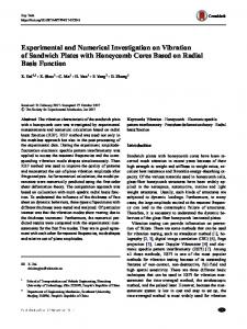
Fig. 17 Turbine rpm versus towing speed in free loading condition. Following the procedure explained so far, series of tests are conducted for the TSR ranging from 4 to 11. Different sets of rpm are also used for the same TSR to check the Reynolds number effect. Fig. 18 shows all the results keeping the focus placed on the Reynolds number effect. The first, the second and the third rows are for Case 1, Case 2 and Case 3 turbines, respectively, and the first, the second and the third columns are for the power coefficient, the torque coefficient and the measured torque, respectively. Three different rpms are used for each experiment so that the Reynolds numbers with different rpms for one TSR are different. Due to the limitation of the equipment and the facility, the variation in Reynolds number is not large though. Roughly speaking, the highest Reynolds number with the rpm around 400 is about 3.8×105 over the tested TSR range and the lowest is about 2.0×105. So it is safe to say that the flow regimes are mostly laminar, about to reach the turbulence transition. For all three cases (all three rows) the Reynolds number effect on both dimensionless coefficients is somewhat noticeable for higher TSR and the efficiencies are better for higher Reynolds number in general. However, the effect becomes minor around TSR 5.0 where the maximum efficiency is obtained (and also expected from the CFD). For higher TSR, the flow around the foil is more attached to the foil, and the more Reynolds number dependent friction over the foil surface does an important role. On the other hand, where TSR is around 5.0, the rotation of the turbine is somehow restricted by the extra torque and the flow around the foil is more like stalled flow due to the increased angle of attack, where the less Reynolds number dependent form drag plays a significant role instead.

252


Fig. 18 Measured turbine characteristics as functions of TSR with different sets of rpm to check Reynolds number effect. Case 1, 2 and 3 from top to bottom. Cp, CQ and Q from left to right. Fig. 19 is shown to compare each turbine’s performance at different Reynolds number range. As mentioned earlier the Reynolds number varies over 2.0~3.8×105, depending on the rpm and the towing speed. In the figure, the data is grouped for three different speed ranges and presented in the first (0.9~1.9 m/s), the second (1.1~2.4 m/s) and the third (1.4~3.0 m/s) columns as functions of TSR. The power coefficients of Case 2 and 3 are considerably larger than Case 1 over the whole TSR range, and Case 3 seems better than Case 2 by a slight margin, regardless of the Reynolds number differences. At the design TSR 5.17, Case 2 is 3.464% better and Case 3 is 6.67% better compared to Case 1 in the power coefficient CP based on the highest Reynolds number results. As a summary, the measured power coefficients for the three cases are shown in Fig. 20, together with the CFD values


253

discussed in the previous section. The turbines designed in this study are giving their best performances at their design TSR and the two cases (Case 2 and 3) developed with the consideration of the tidal current characteristics are showing better efficiency than Case 1. The Case 3, adopted the tip rake considering the cavitation issue, not only helps to reduce the tip vortex but also provides the highest efficiency 0.45. The experiments support all the arguments made with the computations, but there still exists some quantitative discrepancies between those two, most probably due to the Reynolds number difference. Compared to the CFD’s highest CP for Case 3 (0.489), the highest experimental CP is 8.0% lower. In this experimental study, no additional effort is made to look at possible cavitation inception.

Fig. 19 Comparison of the performance of three blades, Cases 1, 2 and 3 at different Reynolds number ranges. The first and the second rows are CP and CQ, respectively. The 1st column is with the towing speed 0.9~1.9 m/s, the second column with 1.1~2.4 m/s and the third column with 1.4~3.0 m/s.

Fig. 20 Measured and computed power coefficients for the three turbines.

254


CONCLUSIONS Three types of tidal stream turbines are proposed and their performance is studied both numerically and experimentally. The target is set to provide 100 kW power from a three-bladed turbine of 8 m diameter in 2 m/s current. Following a standard wind turbine design procedure a base blade is derived, and two additional blades are proposed with more focus on efficiency and cavitation. Similarly to common wind turbines, the base turbine is composed of two foils; a thicker DU-93-W210 section toward the hub and a thinner NACA63-418 section toward the tip, and the root is circular cylinder. The second turbine uses the more efficient NACA foil for the whole span and its root is replaced with an elliptic cylinder. This proposition is reasonable since tidal currents are much smoother and very predictable compared to the wind. The third blade adopts a tip rake aiming at mitigating the strong tip vortices which usually accompany cavitation. For the three designed turbines, numerical simulations are carried out by using a commercial CFD code, FLUENT. The calculations show that their efficiencies reach their maxima (around 49%) at the tip speed ratio (TSR) 5.17 which is near the design condition. The calculations predict that the two newly designed turbines perform better than the base turbine. The simulation also shows that the tip vortex existing on the second type blade is actually reduced for the third turbine with a tip rake and the minimum allowable depth without cavitation is smaller. Moreover, the turbine with a tip rake gives better efficiency as well than the second turbine. The performance of the three turbines is experimentally investigated also in a towing tank. The model diameter is 700 mm and the Reynolds number ranges in 2.0~3.8×105 for the interested TSR. The experimental results also show that the third turbine with tip rake gives the best efficiency among three designed turbines and the second turbine is better than the first one in efficiency which is qualitatively same as computational results although there is large difference in Reynolds number between them. In order to understand the limitation of the experiment, stemming from the Reynolds number discrepancy, the scale problem is carefully investigated with the given circumstances. All the prediction made in the CFD is verified by the model experiment, while there still are some considerable quantitative differences between the two. The highest efficiency from the experiment is 45%, which is 8.16% less than the numerical prediction.

ACKNOWLEDGEMENTS This work was supported by the Ministry of Knowledge Economy through KETEP under the contracts 20093021070010 and 20093020070020 and National Research Foundation of Korea (NRF) grant funded by Korea government (MEST) through GCRC-SOP No.2011-0030660.

REFERENCES Bahaj, A.S., Molland, A.F., Chaplin, J.R. and Batten, W.M.J., 2007. Power and thrust measurements of marine current turbines under various hydrodynamic flow condition in a cavitation tunnel and a towing tank. Renewable Energy, 32(3), pp.407-426. Baltazar, J. and Falcao de Campos, J.A.C., 2009. Unsteady analysis of a horizontal axis marine current turbine in yawed inflow conditions with a panel method. 1st International symposium on marine propulsors. Trondheim, Norway. Burton, T., Share, D., Jenkins, N. and Bossanyi, E., 2001. Wind energy handbook. John Wiley & Sons. Drela, M., 1989. XFOIL: An Analysis and Design System for Low Reynolds Number Airfoils. MIT Dept. of Aeronautic and Astronautics, Cambridge, Massachusetts. [Accessed 3 October 2011]. Hyundai Heavy Industries co., ltd., 2000. Propeller with curved rake pattern at the tip region. Korea. Pat. 1003944860000. ITTC, 2002. Propulsion, propulsor uncertainty analysis, example for open water test. ITTC-recommended procedures and guidelines. 7.5-02-03-02.2. Jo, C.H., Kang, H.L. and Rho, Y.H., 2010. Recent TCP (Tidal Current Power) projects in Korea. Science China Technological Sciences, 53(1), pp.57-61. Kim, S.E. and Choudhury, D., 1995. A near-wall treatment using wall functions sensitized to pressure gradient. In: M. Outgen et al., ed. 1995. ASME FED Separated and Complex Flows, 217, pp.13-18. August, Hilton Head, SC, USA. Kinnas, S.A. and Xu, W., 2009. Analysis of tidal turbines with various numerical methods. 1st annual MREC technical conference. MA, USA.


255

Rourke, F.O., Boyle, F. and Reyolds, A., 2010. Marine current energy device: current status and possible future applications in Ireland. Renewable and Sustainable Energy Reviews, 14(3), pp.1026-1036. Sauser, B., 2008. Tidal Power Comes to Market. Technology Review. [online] Available at: [Accessed 14 January 2012]. Shih, T.H., Liou, W.W., Shabbir, A., Yang, Z.G. and Zhu, J., 1995. A new kappa-epsilon eddy viscosity model for high Reynolds-number turbulent flows. Computers and Fluids, 24, pp.227-238. Stern, N., 2007. The stern review, the economics of climate change. Cambridge: Cambridge University Press. Weiss, J. and Smith, W., 1995. Preconditioning applied to variable and constant density flows. AIAA Journal, 33(11), pp. 2050-2057.