uate students and colleagues who have made important contributions: Joel .... for Einstein's equations coupled to dust which tracks Oppenheimer-Snyder ...
Numerical Asymptotics ´ R. GOMEZ AND J. WINICOUR DEPARTMENT OF PHYSICS AND ASTRONOMY, UNIVERSITY OF PITTSBURGH, PITTSBURGH, PA 15260 We review the present status of the null cone approach to numerical evolution being developed by the Pittsburgh group. We describe the simplicity of the underlying algorithm as it applies to the global description of general relativistic spacetimes. We also demonstrate its effectiveness in revealing asymptotic physical properties of black hole formation in the gravitational collapse of a scalar field. 1 INTRODUCTION We report here on a powerful new approach for relating gravitational radiation to its matter sources based upon the null cone initial value problem (NCIVP), which has been developed at the University of Pittsburgh . We are grateful to the many graduate students and colleagues who have made important contributions: Joel Welling (Pittsburgh Supercomputing Center), Richard Isaacson (National Science Foundation), Paul Reilly, William Fette (Pennsylvania State University at McKeesport) and Philipos Papadopoulous. As will be detailed, the NCIVP has several major advantages for numerical implementation. (i) There are no constraint equations. This eliminates need for the time consuming iterative methods needed to solve the elliptic constraint equations of the canonical formalism. (ii) No second time derivatives appear so that the number of basic variables is half the number for the Cauchy problem. In fact, the evolution equations reduce to one complex equation for one complex variable. The remaining metric variables (2 real and 1 complex) are obtained by a simple radial integration along the characteristics. In null cone coordinates, Einstein’s equations form a system of radial differential equations which can be integrated in hierarchical order for one variable at a time. We have been able to utilize this structure to construct a marching algorithm in which evolution to the next grid point is carried out with no extra computational baggage such as iterative procedures or inversion of matrices. (iii) The radiation zone can be idealized as a finite grid boundary using the Penrose compactification technique (Penrose 1963) for null infinity. No extraneous outgoing radiation conditions are required at null infinity, which both in theory and in practice acts as a perfectly absorbing boundary. This allows the rigorous description of radiation in terms of geometrical quantities such as the Bondi mass and news function (Bondi et. al. 1962),
the angular momentum and supermomentum associated with the asymptotic symmetry group (Winicour 1989), and the Newman-Penrose conserved quantities (Newman & Penrose 1968). It supplies the waveform and the polarization incident on a distant antenna. Because of the singular time behavior of the compactified version of spatial infinity (Ashtekar & Hansen 1978), the analogous approach to the Cauchy problem is not practical numerically. Instead, the grid is terminated at some radius R, where an outgoing radiation condition must be imposed. There do not exist specific estimates of the effect of such boundary conditions on the interior physics, e.g. by reflection of waves off the boundary. Furthermore, combined with gauge ambiguities, use of a finite grid boundary complicates the extraction of the true wave profile seen by distant observers, who are essentially at null infinity. Although this has been effectively accomplished for the radiation from axially symmetric perturbations of relativistic stars (Abrahams & Evans 1990) it becomes much more problematical in the highly nonlinear and asymmetric case. (iv) The grid domain is exactly the region in which waves propagate, which is ideally efficient for radiation studies. Since each null cone extends from the source to null infinity, we see the radiation immediately with no need for numerical evolution to propagate it across the grid. Furthermore, in the case of black hole formation, the exterior region of spacetime which is of physical interest is itself bounded in the future by a null hypersurface which forms the horizon associated with the final black hole state. Here the use of null hypersurfaces again leads to an efficient choice of grid domain, although in highly asymmetric systems, such as two coalescing black holes, the caustic structure of the horizon is expected to be much more complicated than that of a null cone. There are also disadvantages of the NCIVP. (i) One is the issue of caustics. A null cone is a special type of null hypersurface in which the caustics consist of a single spacetime point. In gravitational systems with large asymmetry, the focusing effect can lead to more complicated caustic structure and preclude the existence of null cones. Although there are methods to include arbitrary caustics in the characteristic initial value problem (Friedrich & Stewart 1983), at the present developmental stage we prefer to avoid this issue. In analogy with geometric optics, it is not the lensing effect of strong curvature by itself which leads to caustics but also the location of the lens with respect to the vertex. In a spacetime with negligible curvature containing, say, two peanuts, no global null cones exist if the peanuts are sufficiently far apart (approximately 1010 light years). On the other hand, in spacetimes with strong curvature, global null cones exist (or end on true physical singularities) in the case of near spherical symmetry and even for a binary neutron star system with orbital separation of less than 5 neutron star radii. It is known from the geometric optics approximation that gravitational lensing by an intermediary object between the source and observer can enhance the detectability of gravitational radiation in the same manner as for
electromagnetic radiation, although this is likely to be too fortuitous to be of practical value. However, there is also another qualitatively different form of lensing which occurs when the “focal length” is matched to the size of the dynamical radius of the source. This occurs in the case of binary neutron stars at the minimal orbital radius that admits global null cones and it is generic of binary black holes. It is not known to what extent this dynamical lensing might enhance the detectability of gravitational radiation from these binary systems. This is an effect for which standard perturbation theory based upon harmonic light cones cannot be trusted and which has not yet been investigated numerically. (ii) The Courant stability condition requires that the physical domain of dependence be smaller than the domain of dependence determined by the numerical algorithm. For an explicit finite difference algorithm, this places a stronger restriction on the size of the time step near the vertex of the null cone than occurs for the Cauchy problem (G´omez, Isaacson & Winicour 1992). This can be circumvented by using either an implicit algorithm or a variable grid but again, at the present developmental stage, we prefer to keep the algorithm as simple as possible in finite difference form for purposes of calibration. (iii) Although the technique of shooting along characteristics is common in computational mathematics, there is very little history for the numerical implementation of the characteristic initial value problem. Outside of work done in general relativity, the literature only treats systems with one essential spatial dimension. This makes it prohibitive to try to develop an astrophysically realistic hydrodynamic code along with the gravitational code. (iv) There is a paucity of exact solutions that can be expressed in null coordinates for use in code calibration and debugging. One is the Oppenheimer-Snyder solution. In collaboration with W. Fette, we have developed a spherically symmetric code for Einstein’s equations coupled to dust which tracks Oppenheimer-Snyder collapse, to second order accuracy in grid size, through the horizon up to the formation of the singularity. However, until recently, there were no nonspherically symmetric metrics known in null cone coordinates, other than the Minkowski metric, that were sufficiently global to serve as a test bed. This requirement is intrinsically more difficult than in the Cauchy problem, where the domain of dependence of a small portion of the initial spacelike hypersurface is nonempty, so that evolution can be tested locally by avoiding the singular regions of the exact solution. In the case of a null cone, the domain of dependence is empty for any portion not containing the vertex. Following a suggestion of J. Bicak, we developed a null cone formulation of the boost-rotation symmetric spacetimes (Bicak, Reilly & Winicour 1988). In further work with Reilly, we have used this formalism to find the only known nonflat vacuum spacetime that can be analytically expressed in null coordinates with a nonsingular vertex. This provides an important test bed for code development.
2 THE NULL CONE FORMALISM Figure 1 illustrates how null cone coordinates xµ = (u, r, xA ) are uniquely determined (up to a trivial angular coordinate freedom) by a point O and a timelike vector T µ in its tangent space. These determine a timelike geodesic which serves as the origin worldline for the vertices of a family of null cones. Let the coordinate u be the proper time along this geodesic, with u = constant on the outgoing null cones. Let xA (A = 2, 3) be coordinates for the outgoing null rays, consistent with parallel propagation along the origin worldline. Let r be a surface-area distance on the null cones. Then, in the corresponding Bondi coordinate system, the line element takes the form ds2 = Hµ dxµ du − r2 hAB dxA dxB , (1) where, for numerical purposes we choose xA = [−cos(θ), φ] in terms of the usual polar coordinates. Then det(hAB ) = 1. Also, the numerical grid is based upon the compactified radial coordinate x = r/(1 + r), so that points at future null infinity J+ are included in the grid at x = 1. The coordinate conditions at the origin imply that the metric reduces to a Minkowski (null polar) form along the central worldline. However, the resulting metric does not take an asymptotic Minkowski form at J+ . Initial null data for the gravitational field consists of the 2-metric hAB . Because of the unimodular condition, this entails two degrees of freedom describing the conformal 2-geometry of the surfaces of constant r on the initial nullcone. It is convenient to introduce a complex polarization dyad hAB = 2m(A m ¯ B) .
(2)
Then these dynamical degrees of freedom can be efficiently described in terms of the single complex function ζ = m3 /m2 . There is a one-to-one correspondence between choices of ζ and symmetric unimodular matrices hAB . There are no constraints on this data except that it be consistent with smoothness at the origin and asymptotic flatness. The vacuum field equations consist of four hypersurface equations for Hµ and one complex evolution equation for ζ. They take the symbolic form Z
H1 = HA =
Z0 r 0
Z
H0 =
r
0
(3)
drJA [ζ, H1 ]
(4)
drJ0 [ζ, H1 , HA ]
(5)
drJ[ζ, Hµ ].
(6)
r
Z0 r
∂ζ/∂u =
drJ1 [ζ]
Here the the J-operators consist of explicit operations intrinsic to the null cone. These equations form a hierachy which leads from the initial data ζ to its time derivative by means of a series of radial integrations. Our first attempt at a numerical code for axisymmetric vacuum space-times based upon the null cone algorithm led to unexpected difficulties. The numerical grid included null infinity as a compactified boundary and yielded the first successful numerical calculations of the Bondi mass and news function for gravitational waves (Isaacson, Welling & Winicour 1983). However, near the vertex of the null cone, instabilities arose which destroyed the accuracy of the code over long time scales. We felt that this problem was too complicated to analyze in the context of general relativity, considering that the numerical analysis of the characteristic initial value problem had not yet been carried out even for simplest linear axisymmetric systems.
u
u
+ J
J+ T Q
x
T
A r
P u + du 0
u
r=0
x=1 u=u
S
R
0
O
u
r=0
Fig. 1 Null cone coordinates.
0
Fig. 2 Scheme for the marching algorithm.
3 THE FLAT SPACE WAVE EQUATION This warranted an investigation of the basic mathematical properties of the numerical evolution of the flat space scalar wave equation using a null cone initial value formulation (G´omez, Isaacson & Winicour 1992). Consider the scalar wave equation Φ = N L + S,
(7)
where the terms on the right hand side represent a nonlinear potential, such as a Φ4
potential, and an external source. This can be reexpressed in the form (2)
g=−
L2 g + r(N L + S), r2
(8)
where g = rΦ and L2 is the angular momentum operator. Integration over a null parallelogram in the (u, r)-plane as depicted in Fig. 2, leads to the integral equation 1Z L2 g gQ = gP + gS − gR + dudr[− 2 + r(N L + S)]. 2 A r
(9)
This identity gives rise to an explicit marching algorithm for evolution. Let the null parallelogram span null cones at adjacent grid values u0 and u0 + ∆u, as shown in Fig. 2, for some θ and φ. Imagine for now that the points P , Q, R and S lie on the grid, so that xQ − xP = xS − xR = ∆x. If g has been determined on the entire u0 cone and on the u0 + ∆u cone radially outward from the origin to the point P , then (9) determines g at the next radial grid point Q in terms of an integral over A. The integrand can be approximated to second order, i.e. to O(∆x∆u), by evaluating it at the center of A. To the same accuracy, the value of g at the center equals its average between the points P and S, at which g has already been determined. After carrying out this procedure to evaluate g at the point Q, the procedure can be repeated to determine g at the next radially outward point, the point T in Fig. 2. After completing this radial march to null infinity, the field g is then evaluated on the next null cone at u0 + 2∆u, beginning at the vertex where smoothness gives the start up condition that g = 0. The resulting evolution algorithm is a 2-level scheme which reflects, in a natural way, the distinction between characteristic and Cauchy evolution, i.e. that the time derivative of the field is not part of the characteristic initial data. In practice, the corners of the null parallelogram, P , Q, R and S, cannot be chosen to lie exactly on the grid because the velocity of light in terms of the compactified coordinate x is not constant even in flat space. As a consequence, the field g at these points is approximated to second order accuracy by linear interpolation between grid points. However, cancellations arise between these four interpolations so that (9) is satisfied to fourth order accuracy. The net result is that the numerical version of (9) steps g radially outward one cell with an error of fourth order in grid size. Second order global accuracy is indeed confirmed by convergence tests of the code. For sufficiently large r, we found from an analysis of domains of dependence that the Courant limit on the step size is the same as for a standard Cauchy evolution in spherical coordinates, ∆u < 2∆r (10)
and ∆u < r∆θ.
(11)
However, near the origin, this analysis gives a much stricter limit ∆u < Kr(∆θ)2 ,
(12)
where K ≈ 1. These stability limits were confirmed by numerical experimentation. Operating within this Courant limit, the algorithm has been implemented as a stable, calibrated, globally second order accurate evolution code on a compactified grid (G´omez, Isaacson & Winicour 1992). Numerical evolution accurately satisfies the mass-energy flux conservation law. Furthermore, null infinity behaves as a perfectly absorbing boundary so that no radiation is reflected back into the system. This algorithm offers a powerful new approach to generic wave type systems. By constructing an exact nonspherical solution for a Φ4 potential, we were able to calibrate the algorithm in the nonlinear case. It tracked the solution with the predicted second order accuracy right up to the formation of physical singularities. By other choices of potential, we were able to study approximate axisymmetric versions of solitary wave phenomena. The basic algorithm is applicable to any of the hyperbolic systems occurring in physics. 4 SELF-GRAVITATING SCALAR WAVES. We subsequently extended this algorithm to self-gravitating, spherically symmetric, zero-rest-mass scalar waves, as described by the Einstein-Klein-Gordon equation (G´omez & Winicour 1992a). 1 Gµν = 8π[∇µ Φ∇ν Φ − gµν ∇α Φ∇α Φ]. 2
(13)
In null cone coordinates, the line element takes the Bondi form V ds2 = e2β du( du + 2dr) − r2 (dθ2 + sin2 θdφ2 ). r
(14)
Let H(u) = β(u, ∞). Then Bondi time u ˜ , measured by inertial observers at null infinity, is related to central time by d˜ u = e2H . du
(15)
Horizon formation occurs at a finite central time u = uH but at an infinite Bondi time u ˜ H = ∞. In the case of spherical symmetry, g = rΦ obeys a two dimensional wave equation intrinsic to the (u, r) plane. In two dimensions, the geometry is conformally flat, the
wave operator has conformal weight -2 and the surface area element has conformal weight +2, so that the surface integral of (2) g over a null parallelogram gives exactly the flat space result. This allows use of the same basic evolution algorithm already described. The only new feature is that the radial integration of the hypersurface equations must be worked into the algorithm to determine β(u, r) and V (u, r). 4.1 Asymptotic Properties Christodoulou (Christodoulou 1986a, 1986b, 1987a, 1987b) has made a penetrating analysis of the existence and uniqueness of solutions describing gravitational collapse of a scalar field, in the spherically symmetric scalar case, and has established a rigorous version of a no-hair theorem. He proved that weak initial data evolves to Minkowski space asymptotically in time but that sufficiently strong data forms a horizon, with nonzero final Bondi mass MH . The geometry is asymptotically Schwarzschild in the approach to I + (future timelike infinity) outside the sphere r = 2MH . Figure 3 depicts the spacetime of such a field beginning at initial retarded time u0 and forming a horizon at uH . The situation differs from Oppenheimer-Snyder collapse in that the backscatter of radiation causes the r = 2MH curve to intersect the horizon only in the asymptotic limit at I + . In that respect, it is more akin to the spacetime of a dust distribution whose interior collapses but whose exterior escapes to infinity, as depicted in Fig. 4. X
I+
X
X X X
X
X
X
X
X
J+
X
r=0
u H
X
X
X
J+ Schwarzschild
Dust
r= 2MH
r=2M
r=0
Fig. 3 Gravitational collapse of a scalar field.
X
r=0
u H
u0
I+
X
r=0
u0
Fig. 4 Collapsing-expanding dust.
When a horizon forms, Christodoulou’s no hair theorem states that the geometry has the asymptotic step function behavior ( 2(β−H)
e
→
0 for r < 2MH 1 for r > 2MH
(16)
in the limit u → uH . From the hypersurface equation β,r = 2πr(Φ,r )2 ,
(17)
it follows that Φ → 0 as u → uH for r > 2MH . The compactified grid allows the accurate tracking of the scalar radiation field right up to time infinity I + . In the curved space case, the Courant condition requires that the ratio of the time step size to radial step size be limited by (V /r)∆u ≤ 2∆r, where ∆r = ∆[x/(1 − x)]. The strongest restriction arises at J + , just before the formation of a horizon. In this limit, V /r → ∞ so that the conformal singularity at I + freezes the numerical evolution. The code becomes unreliable when the red shift between central time and Bondi time is of the order of 109 . In order to evolve across the horizon, exterior radial points must be dropped from the domain of the grid. Figure 5 illustrates the formation of a step function just before horizon formation during a typical numerical evolution, in confirmation of Christodoulou’s theorem. One static solution for a spherically symmetric, self gravitating zero rest mass scalar field is Φ = constant, which is pure gauge and not by itself physically interesting. Another is the analog of the static solution Φ = 1/r in a Minkowski background (Janis, Newman & Winicour 1968). Pasting these together gives rise to initial data whose evolution is not static because of the jump discontinuity in the curvature at their interface. This gives rise to a shock front along a radially incoming characteristic. Results of a numerical evolution of g(x, u) are shown in Fig. 6 for the case of initial amplitude large enough to form a horizon. To the past of the shock front, Φ remains constant. Although g(x, u) = rΦ has a curved profile in this region, the evolution is manifestly static. The numerical code clearly handles the inward propagation of the shock front without difficulty. Outside the shock front, backscattering distorts the initial profile. This distinctly illustrates the breakdown of Huyghen’s principle due to curvature. The numerical code handles the propagation of the shock front without any substantial difficulty. It introduces some slight high frequency numerical noise just outside the shock front, but too small to be perceptible in the figure.
Fig. 5 Formation of a step function.
Fig. 6 Evolution of static-static data.
Fig. 7 Decay of the monopole mopment. Fig. 8 The initial data for a wave train. The early stage of the evolution appears innocuous but then the outer region of the profile flattens. This marks the beginning of the process of “shedding hair” as a black hole starts to develop. As this process intensifies in the late stage, a cusp begins to
form near r = 2MH , which corresponds to the conformal singularity developing at I + . Note that the slope of g at J + is conserved during the evolution. It is an example of a Newman-Penrose conserved quantity. Our results demonstrate how the NewmanPenrose constant is indeed conserved while remaining consistent with the no hair scenario. The time dependence of the monopole moment Q(u) = g(u, ∞) is graphed in Fig. 7. After a long dive to a negative value, it bobs up abruptly to zero just before the horizon forms. The numerical evolution is stopped just short of the horizon due to the inability of the grid to resolve the cusp. The redshift factor at this time is d˜ u/du ≈ 107 . Careful inspection of the numerical results shows that its final decay √ has time dependence uH − u. From recent discussions with P. Rabier and W. Rheinboldt, we have learned that this corresponds to a canonical singularity in the general theory of Differential Algebraic Equations (DAE’s) (Rabier 1989; Rheinbolt 1984), in which a quantity has a well defined limit but its time derivative does not. We find that central time and Bondi time are related asymptotically by uH − u ∼ e−˜u/4MH , 4MH
(18)
analogous to the relation between Kruskal and Schwarzschild times. This implies that the monopole moment decays exponentially in Bondi time, in contrast to the power law predicted by perturbation theory in an Oppenheimer-Snyder background (Price 1972). This is surprising since in this final phase the metric is very close to a Schwarzschild metric in the region exterior to r = 2MH . Another illustrative example is provided by the strong amplitude initial data given in Fig. 8. Figure 9 graphs g just before horizon formation in a strong amplitude case; and Fig. 10 graphs what would be the linear evolution of g at a suitable time for comparison with the strong amplitude graph. The qualitative difference between these graphs highlights the nonlinear effects of self gravitation. The most striking feature of the strong amplitude case is that the horizon forms quite insensitively to the detailed structure of the field in the inner region r < 2MH . The chief difference, between the strong and weak case, in the evolution of g inside this inner region arises from the way in which the outgoing wave from the origin interferes with the incoming signal. In the weak case this interference lowers the entire profile in Fig.10 by a constant determined by the amplitude of the outgoing wave leaving the origin at that time. In the strong case, backscattering couples the the incoming and outgoing waves. The linear slope modulating the wave profile in Fig. 9 is a prime illustration of backscattering depleting the outgoing wave.
Fig. 9 Strong amplitude evolution.
Fig. 10 Weak amplitude evolution.
4.2 Scaling Limits The Bondi mass of this Einstein-Klein-Gordon system has some remarkable asymptotic behavior with respect to the one parameter family of data obtained from the amplitude rescaling Φ(u0 , r; λ) = λΦ(u0 , r), which preserves asymptotic flatness. By an application of the method of Laplace, we have derived the following asymptotic formula for large λ which holds when the monopole moment is nonvanishing, π M (u0 ; λ) ∼ √ |Q(u0 ; λ)|. 2
(19)
In this regime, the mass is essentially the magnitude of the monopole moment and scales linearly with λ! Compare these results to the small amplitude regime, in which M depends quadratically on λ. In the strong field case, a redshift type effect weakens the dependence of M on the the inner region of the matter distribution and the dominant contribution comes from the far field monopole moment. The details of the transition from the low amplitude to high amplitude asymptotic regimes can be obtained from numerical calculations of the mass using our code. The result for a typical choice of data is illustrated in Fig. 11. The transition from quadratic to linear λ dependence occurs around the critical value λc , at which the evolution bifurcates between forming or not forming a horizon. For data of compact support within a radius R, the method of Laplace leads to the
high amplitude asymptotic dependence M (u0 ; λ) ∼ R/2.
(20)
In this case, redshifting completely saturates the λ dependence and the null data approaches that for a horizon at R = 2M . This is illustrated in Fig. 12. The study of a specific analytic model (Winicour 1990) with compact null data also shows that the news function is completely redshifted away, N (λ) → 0 as λ → ∞ holding R constant. Amplitude scaling, does not commute with evolution, Φ(u1 , r; λ) 6= λΦ(u1 , r), except in the small λ linearized limit. This lies behind the somewhat magical way in which high amplitude noncompact data, with large M and Q, rapidly sheds its monopole moment, along with its exterior field, without significant mass loss as a black hole forms.
Fig. 11. Scaling of the Bondi mass for nonvanishing monopole moment.
Fig. 12. Scaling of the Bondi mass for compact data
Another global quantity with interesting properties is Z
∞
P = 4π 0
r(g,r )2 dr.
(21)
P 1/2 , like the square root of the Bondi mass, provides a norm on the vector space of asymptotically flat initial data. P scales quadratically with respect to λ under amplitude rescaling. It is implicit from the results of Christodoulou that its derivative with respect to Bondi time can be expressed in the form P,˜u = M − λ∂λ M.
(22)
In the linear regime, the Bondi mass scales quadratically so that λ∂λ M ∼ 2M and (22) reduces to P,˜u ∼ −M . Thus P must monotonically decrease in the weak field regime. This explains how flat spacetime arises as a basin of attraction for the weak field case. Since during the formation of a horizon the field develops compact support within a radius 2MH , one would expect that ∂λ M → 0 and therefore that P,˜u ∼ MH ,
(23)
These late time asymptotics can also be confirmed by numerical evolution, as illustrated in Fig. 13.
Fig. 13. Comparison of P,˜u and M .
Fig. 14. Scaling of P.
Figure 14 plots P (˜ u) for several representative values of λ. Many qualitative features of these graphs can be explained in terms of asymptotic results previously discussed. For the two graphs with λ < λc , P decays to zero as the system decays to flat space, in keeping with the role of P as a norm. For the three graphs with λ > λc , P exhibits interesting asymptotic behavior. First, at the initial time u ˜ = 0, these three graphs of P all have approximately the same slope. This is a manifestation of the high amplitude scaling properties which can be established for dP/d˜ u (G´omez & Winicour 1992a). The numerical results show that the high amplitude limit remains a good approximation to 10% accuracy even for values λ ≈ λc . At large Bondi time, these three graphs again tend toward straight lines exhibiting the asymptotic relation dP/d˜ u → MH . From the asymptotic slope of these graphs, it is evident that systems which start out at higher amplitude develop horizons with greater mass.
Fig. 15. Behavior of P near critical data. Fig. 16. Comparison of profiles at R = 25M (dashed line) and J + (solid line) for compact initial data. Figure 15 plots P (˜ u) for values of λ just above and just below the critical value of the amplitude. The bumpy features in the graph may be a rough version of the intricate structure that appears in the neighborhood of the critical value, which has been described by Choptuik (Choptuik 1989). The graph also clearly shows the value of P as a diagnostic tool for determining the fate of the system at large times. 4.3 Collapse Criteria Christodoulou (to appear) has established a condition on the initial data for the scalar field which is sufficient to guarantee collapse to a black hole. It is based upon pairs of spheres along the initial null cone with radii (r1 , r2 ) (measured by surface area) and upon the Hawking masses (m1 , m2 ) of these spheres. For a given pair, let r2 − r1 r1
(24)
2(m2 − m1 ) . r2
(25)
δ := and η :=
Then a horizon forms if there is a pair which satisfies the inequalities 0 Hc , where Hc is independent of the choice of data? 4.4 Waveforms at Finite Distances We have also used the spherically symmetric, massless Einstein-Klein-Gordon system to investigate the discrepancies that arise if waveforms are observed at a grid boundary with finite radius R, as opposed to null infinity (G´omez & Winicour 1992b). For a system of mass M > M for sufficiently periodic systems. They are most pronounced for radiation losses between one quarter and one half of the initial mass. This falls within the expected regime of the spiral infall of a relativistic binary system. The predominant contribution to this discrepancy stems from a time dependent redshift arising from radiative mass loss. For gravitational waves, there are severe complications which can potentially affect the accuracy of waveforms based upon a finite worldtube. Gauge ambiguities make it unclear which components of the metric or curvature tensor to use. Some method of selecting the components transverse to the propagation direction is necessary but there is no unique means of defining this propagation direction locally. The choice of time coordinate can introduce further gauge effects. There are additional physical complications. Time dependent versions of redshifting occur. The nonlinear gravitational self-source is noncompact and introduces backscattering which blurs the distinction between incoming and outgoing fields. A finite grid boundary also leads to some backscatter. Furthermore, in a case such as a binary black hole system, there is no practical scheme for eliminating incoming waves from the initial data. In spite of these complications, techniques used by numerical relativists with spacelike codes have led to consistent and sensible results in the range of problems where they have been applied (neutron star oscillations, supernovae). The spherically symmetric scalar model has no ambiguity in the local radial direction and no other gauge ambiguities. Furthermore, initial incoming waves are eliminated in the test region by choosing initial data with compact support. In the nonspherical case, this remedy is not possible for the initial data describing gravitational degrees of freedom because of the constraint equations. Elimination of these effects allows isolation of the nonlinear effects of backscattering and time dependent redshifting. Furthermore, spherical symmetry allows the luxury of a very fine grid so that these effects can be studied without contamination by numerical noise. The radiation amplitude at J + is Q(˜ u) = g(˜ u, ∞), where the Bondi time u ˜ plays the role of the proper time used by an observer at infinity. As the counterpart of Q(˜ u) based upon the worldtube, we choose q(τ ; R) = g(˜ u(τ, R), R), where τ = τ (˜ u, R) is the proper time on the worldtube. There is a relative redshift between observers on the worldtube and at J + . In order to synchronize the two time coordinates we set τ0 = u ˜ 0 = 0 on the initial null cone. We have tested how accurately q(τ ; R) serves as a substitute for Q(˜ u). By construction, the test is automatically satisfied in the linear weak field case throughout any region where the wave is purely outgoing. The
waveform at a finite radius can be very misleading when incoming waves are present. In strongly nonlinear fields, there is no clean way to decompose the wave into incoming and outgoing parts. But to make the test clear cut, we will only consider initial data with support r < 1 and test radii R ≥ 1 at which q(τ ; R) measures only the outgoing radiation and the backscattering. In order to quantify the discrepancy between the waveform q and the radiative waveform Q we use the l2 norm and the figure of merit E=
||q − Q|| . ||Q||
(29)
Since the l2 norm is independent of basis, the same error applies to the fourier transform of the signal. The strategy here is to choose initial data characterized by two parameters, representing amplitude and wavelength, and to investigate the resulting waveforms over a comprehensive range. E is small for small amplitudes, in accord with the weak field limit. It is also small at high amplitudes for which a black hole forms very rapidly. This stems from a rigorous version of the no-hair theorem (Christodoulou 1987b) which establishes that the scalar field must vanish in the limit τ → ∞, r > 2MH . As a result, in the region of observational interest, the field is zero initially by construction and, in the high amplitude regime, it never builds up any appreciable amplitude before the interior region collapses to a black hole. Systems in this regime would not be readily detectable because of their extreme redshift. We focus our attention on the intermediate amplitude region of greatest physical relevance. As an example of our test, consider the initial data ½
g(u0 , r) =
Λ sin(2πN (r − 1)) for r ≤ 1 0 for r ≥ 1 ,
(30)
where Λ controls the amplitude and N controls the wavelength. The results are graphed in Fig. 16 for the choices N = 20 and Λ = 9.5 × 10⁻⁴ , for which the initial mass is M0 = 0.041 and the system forms a black hole with MH = 0.029. The discrepancy in the waveform at R = 25M0 is E = 0.91. The amplitudes shown in the figure are in close agreement, which indicates very little backscatter in the intervening region. However, there is considerable phase shifting, which results from a time dependent redshift effect, and this is the prime source of the discrepancy between the waveforms. In the same manner, we also find a large discrepancy, E = 0.80, at R = 100M0 by increasing N to 100. High accuracy computer simulations for N >> 100 would require too much computer time to be practical. However the trend we have already
seen for large N can be understood and extrapolated √ in terms of a rough analytic model which leads to the approximation E ≈ 2πnM/ 3R, where n is the number of wavetrains radiated before horizon formation. For the previous case with N = 20 (for which n = 8), this gives better than 10% agreement with the value of E from the numerical evolution. For N = 100 (for which n = 24), there is 2.5% agreement between the formula and the numerical value obtained for E. This provides strong evidence that this formula gives a reliable estimate of E in the large N regime. Thus large waveform discrepancies, E ≈ 1, can arise at any radius for a system of sufficiently high frequency, i.e. n ≈ R/M . 5 GRAVITATIONAL WAVES Our aim is to be able to study asymptotic properties of gravitationally radiating spacetimes with the high level of accuracy achieved for scalar radiation. We are currently incorporating the lessons learned from the scalar algorithm into the evolution code for axisymmetric spacetimes. For axisymmetry, the conformal geometry of the spheres of constant u and r is hAB dxA dxB = e2γ dθ2 + sin2 θe−2γ dφ2 ,
(31)
so that γ represents the entire null datum for the gravitational field. The evolution equation (6) can be reexpressed in the form (2)
ˆ Hµ ], γ = J[γ,
(32)
where (2) is the D’Alembertian with respect to the induced geometry of the (u, r) submanifold and Jˆ again consists only of operations intrinsic to the null cone u = const. This has the identical structure as the scalar wave equation (8), thereby leading to the analogue of the null parallelogram identity (9) and to an explicit marching algorithm for the evolution of γ. The same cancellations in the numerical error from the four sides of the null parallelogram that arise in the scalar case can also be arranged here so that the algorithm should in principle yield a globally second order accurate solution. We expect, subject to the Courant limit (12), that it will be free of instabilities at the origin. It is reassuring to know that progress has also been made in this direction at Southampton (Bishop, Clarke & D’Inverno 1990) and at Cambridge (Stewart, this volume). Although the analysis leading to (12) was based on a 2-level evolution algorithm, the results of the Southampton group seem to imply that (12) also applies to 3-level Adams-Bashworth and Predictor-Corrector algorithms. ACKNOWLEDGEMENTS This work was supported by NSF Grant PHY-8803073. Computer time was provided by the Pittsburgh Supercomputing Center under Grant PHY860023P.
REFERENCES Abrahams,A. M. and Evans, C. R. (1990) Phys. Rev D 42, 2585. Ashtekar, A. and Hansen, R. O. (1978) J. Math. Phys., 19, 1542. Bicak, J., Reilly, P and Winicour, J. (1988) Gen. Rel. and Grav., 20, 171. Bishop, N. T., Clarke, C. J. S. and d’Inverno, R. A. (1990) Class. Quantum Grav. 7, L23. See also the articles by Bishop and d’Inverno in this volume. Bondi, H., van der Burgh, M. G. J., and Metzner, A. W. K. (1962) Proc. R. Soc. London Ser. A 270, 103. Choptuik, M. W. (1989) in Frontiers in Numerical Relativity, eds. Evans, C. R., Finn, L. S. and Hobill, D. W. Cambridge University Press, Cambridge. Also, see article in this volume. Christodoulou, D. (1986a) Commun. Math. Phys. 105, 337. Christodoulou, D. (1986b) Commun. Math. Phys. 106, 587. Christodoulou, D. (1987a) Commun. Math. Phys. 109, 591. Christodoulou, D. (1987b) Commun. Math. Phys. 109, 613. Christodoulou, D. Commun. Math. Phys., to appear. Friedrich, H. and Stewart, J. M. (1983) Proc. R. Soc., A 385, 345. G´omez, R., Isaacson, R. A. and Winicour, J. (1992) J. Comp. Phys., 98, 11. G´omez, R. and Winicour, J. (1992a) J. Math. Phys., 33, 1445. G´omez, R. and Winicour, J. (1992b) Phys. Rev. D, 45, 2776. Isaacson, R. A., Welling, J. S. and Winicour, J. (1983) J. Math. Phys. 24, 1824. Janis, A., Newman, E. T., and Winicour, J. (1968) Physical Review Letters 20, 878. Newman, E. T. and Penrose, R. (1968) Proc. R. Soc. London Ser. A 305, 175. Penrose, R. (1963) Phys. Rev. Lett. 10, 66. Price, R. H. (1972) Phys. Rev.D 5, 2419 Rabier, P. J. (1989) J. Math. Anal. and Appl., 144, 425. Rheinboldt, W. C. (1984) Math. of Comp., 43, 473. Stewart, J. M. in this volume. Winicour, J. (1989) in Highlights in Gravitation and Cosmology, eds. Khembavi, A., Narlikar, J., Vishveshwara, C. and Iyer, B. Cambridge University Press. Winicour, J. (1990) in Proc. of the 3rd Canadian Conf. on Gen. Rel. and Rel. Astrophysics, eds. Coley, A., Cooperstock, F. and Tupper, B. World Scientific Pub., Singapore. p.94.