2
Numerical computation of electromagnetic field for general static and axisymmetric current distribution
3
Toshio Fukushima
1
4 5 6
7
National Astronomical Observatory of Japan / SOKENDAI, 2-21-1, Ohsawa, Mitaka, Tokyo 181-8588, Japan E-mail:
[email protected]
Abstract We developed a numerical method to compute the electromagnetic field of arbitrary static and axisymmetric current distribution. The method (i) numerically evaluates a double integral of the electrostatic and magnetostatic potentials of an infinitely thin ring current by the split quadrature method using the double exponential rules, and (ii) derives the electrostatic field and the magnetostatic induction by numerically differentiating the numerically integrated potentials by the central difference formula. A comparison with the exact solution for a poloidal current distribution with an anisotropic Gaussian damping confirmed the 14- and 9-digit accuracy of the potential and the field/induction computed by the new method.
8
Keywords: axial symmetry; electrostatics; magnetostatics; numerical
9
differentiation; numerical quadrature
10
1. Introduction
11
The computation of the electromagnetic field for a general axisymmetric three-
12
dimensional charge/current distribution is a classic problem in physics and engiPreprint submitted to Journal Computational Physics
July 25, 2017
13
neering (Kellog, 1929; MacMillan, 1930). Indeed, its applications are as wide as
14
(i) the electron and ion optics (Szil´agyi, 1988), (ii) the charged particle accelera-
15
tion (Hamm & Hamm, 2012), (iii) the electron microscopy and spectroscopy (Erni
16
et al., 2009), and (iv) the magnetic coil design (Montgomery & Weggel, 1980). Es-
17
pecially, it is one of building blocks of the plasma physics and controlled nuclear
18
fusion (Kikuchi, 2011; Kikuchi & Azumi, 2015).
19
If the spatial distribution of the static electric charge, ρ (x), and of the static
20
current vector, J(x), are explicitly known, then the electrostatic scalar potential,
21
Φ(x), and the magnetostatic vector potential, A(x), are written as convolutions
22
of these distributions with the Newton kernel, 1/|x − x′ |, (Jackson, 1998, equa-
23
tions (1.17) and (5.32)) as 1 Φ(x) = 4πε0
24
µ0 A(x) = 4π
∫
ρ (x′ ) 3 ′ d x, ′ V |x − x |
(1)
∫
J (x′ ) 3 ′ d x, ′ V |x − x |
(2)
25
where the integration is conducted over all the volume occupied by the charge
26
and/or the current vector, and ε0 and µ0 are the vacuum permittivity and perme-
27
ability, respectively. The associated electrostatic field and the resulting magneto-
28
static induction are expressed as
E(x) =
1 4πε0
∫
( ) (x − x′ ) 3 ′ ρ x′ d x, |x − x′ |3
2
(3)
29
µ0 B(x) = 4π
∫
( ′ ) (x − x′ ) 3 ′ J x × d x. |x − x′ |3
(4)
30
These are nothing but Coulomb’s law and the Biot-Savart law (Jackson, 1998,
31
equations (1.5) and (5.14)).
32
When the charge/current distribution is finitely bounded, the external electro-
33
magnetic field can be expanded in harmonics (Garrett, 1951). However, if the
34
evaluation point x is inside the distributions of the charge or current, on the other
35
hand, the integral expressions, equations (1)–(4), suffer from the algebraic singu-
36
larities. This becomes a serious issue for extended distributions such as encoun-
37
tered in the plasma physics.
38
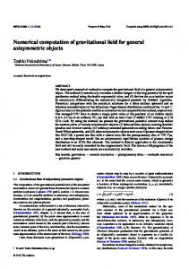
Before going further, let us show a practical example. Fig. 1 shows the con-
39
tour map on a meridional cross section of a hypothetical charge/current distribu-
40
tion. It was designed to resemble the poloidal mode equilibrium solution of the
41
plasma current distribution circulating in an ITER-like tokamak (Evangelias &
42
Throumoulopoulos, 2016, Fig. 4). Refer to Section 4 later for the detailed model
43
description.
44
Although the adopted model distribution is infinitely extended in principle, it
45
can be practically regarded to be finitely bounded thanks to the Gaussian damping
46
around the central ring. Inside this practical boundary, the algebraic singularities
47
appear everywhere. Thus, E(x) and/or B(x) are hardly computed by evaluating
48
the integral forms by the existing quadrature techniques (Press et al., 2007).
49
Therefore, a common practice has been solving Poisson’s equation for Φ(x)
50
and A(x) (Jackson, 1998, equations (1.28) and (5.28)), which are nothing but the 3
Cross Section of Charge/Current 0.75 0.5
z
0.25 0 -0.25 -0.5 -0.75 0 0.25 0.5 0.75 1 1.25 1.5 R Figure 1: Cross section of model electric charge/current distribution. Shown is the contour map on the meridional cross section of a hypothetical electric charge/current distribution. The contours are drawn for the levels of the relative magnitude being inverse powers of 2 as ρ /ρ0 = J/J0 = 2−n for n = 1, 2, . . . , 12. Although the distribution is infinitely extended, it is practically bounded in a finite region thanks to the Gaussian damping feature adopted in the model distribution.
4
51
differential form of Gauss’s and Ampere’s laws, respectively: ∇2 Φ = −ρ /ε0 ,
(5)
∇2 A = −µ0 J.
(6)
52
53
These equations are elliptic type partial differential equations. They are numeri-
54
cally solved by the finite or boundary element methods of various kind (Park et
55
al., 1990; Wang & Demerdash, 1990; Brio et al., 1993; Ma et al., 1996; Le-Van et
56
al., 2016). Refer to Bellina & Serra (2004) for a concise summary of the numer-
57
ical approaches. Nonetheless, the resulting formulation becomes cumbersome in
58
general (Demerdash & Wang, 1990) and suffers from the accuracy degrade (Con-
59
way, 2001). This is especially true if the boundary conditions are complicated
60
(Mitsuoka et al., 2013; Jacques et al., 2016; Mezani et al., 2016).
61
Recently, we developed a numerical method to circumvent the difficulties for
62
the gravitational field of an axisymmetric mass density distribution (Fukushima,
63
2016c). It can be directly applicable to the computation of Φ(x) and E(x) as
64
summarized in Appendix A. Therefore, in this article, we adapt the method to the
65
computation of A(x) and B(x) for arbitrary axisymmetric distribution of electric
66
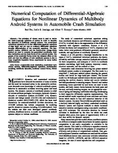
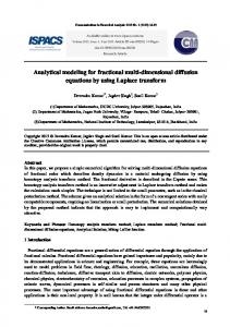
current. By using the original and adapted methods, we prepared Figs 2 and 3
67
showing the bird’s-eye views of E(x) and B(x) of the hypothetical charge/current
68
distribution specified in Fig. 1. As will be shown later, these results are of the
69
9-digit accuracy, which is far more than necessary.
70
Below, we (i) describe the adapted method in Section 2, (ii) examine its com5
Bird’s-Eye View of E E/E0 1 0.5 0.5
0 0 0.5 R
1
z
1.5-0.5
Figure 2: Bird’s-eye view of electrostatic field strength. Displayed is a bird’s-eye view of E ≡ |E(x)|, the magnitude of the electrostatic field caused by the current distribution depicted in Fig. 1.
6
Bird’s-Eye View of B B/B0 1 0.5 0.5
0 0 0.5 R
1
z
1.5-0.5
Figure 3: Bird’s-eye view of magnetostatic field strength. Displayed is a bird’s-eye view of B ≡ |B(x)|, the magnitude of the magnetostatic induction caused by the current distribution depicted in Fig. 1.
7
71
putational accuracy and speed in Section 3, and (iii) present its example in Sec-
72
tion 4.
73
2. Method
74
Consider a general static and axisymmetric current distribution. Adopt the cylin-
75
drical polar coordinate system, (R, z, ϕ ). In this case, the only non-zero compo-
76
nents of J(x) and A(x) are their azimuthal components: J(R, z) ≡ Jϕ (R, z), A(R, z) ≡ Aϕ (R, z).
77
78
(7)
By symmetry, A(x) vanishes on the z-axis as
A(0, z) = 0.
(8)
a(R, z) ≡ A(R, z)/R.
(9)
Therefore, we scale it as
79
Denote the lower and upper end point of the radial distribution by RL (≥ 0) and
80
RU (≤ +∞), respectively. For simplicity, we assume that J(R, z) vanishes when z ≤
81
zL (R) or z ≥ zU (R) where zL (R)(≥ −∞) and zU (R)(≤ +∞) are certain functions of
82
R. Then, a(R, z) is expressed as a double integral convolving J(R, z) with Green’s
83
function as
∫ RU (∫ zU (R′ )
a(R, z) = RL
zL (R′ )
8
) ) ′ F R , z ; R, z dz dR′ , (
′
′
(10)
84
where we abbreviate the integrand as ( ) ( ) ( ) F R′ , z′ ; R, z ≡ f R′ , z′ ; R, z J R′ , z′ ,
85
(11)
while f (R′ , z′ ; R, z) is defined as ( ′ ′ ) ( µ0 ) 16 (R′ )2 S (m (R′ , z′ ; R, z)) f R , z ; R, z = [√ ]3 . 4π 2 2 ′ ′ (R + R) + (z − z)
(12)
86
The function f (R′ , z′ ; R, z) is, except for (i) the multiplier R′ caused by the volume
87
integration element in the cylindrical coordinate system and (ii) the divisor R in-
88
troduced by the scaling, equivalent with the magnetostatic potential evaluated at
89
(R, z) of a uniform ring current located at (R′ , z′ ) (Jackson, 1998, equation (5.37)).
90
In equation (12), m (R′ , z′ ; R, z) is a function defined as [( ( ′ ′ ) )2 ( ′ )2 ] ′ ′ m R , z ; R, z ≡ 4R R/ R + R + z − z ,
91
(13)
while S(m) is a special complete elliptic integral (Fukushima, 2010) defined as S(m) ≡ [(2 − m)K(m) − E(m)] /m2 ,
(14)
92
where K(m) and E(m) are the complete elliptic integral of the first and second
93
kind with the parameter m ≡ k2 , respectively (Wolfram, 2003). Do not confuse m
94
with the modulus k, which has been adopted as the argument of complete elliptic
95
integrals in the classic literature (Byrd & Friedman, 1971; Olver et al., 2010). 9
Complete Elliptic Integrals 5 4.5 4 3.5 3 2.5 2 1.5 1 0.5 0
K(m) E(m) S(m) 0
0.1 0.2 0.3 0.4 0.5 0.6 0.7 0.8 0.9
1
m
Figure 4: Behaviour of complete elliptic integrals. Plotted are the three complete elliptic integrals, K(m), E(m), and S(m) ≡ [(2 − m)K(m) − E(m)]/m2 .
10
96
Refer to Fig. 4 for the behavior of these complete elliptic integrals for the
97
standard domain, 0 ≤ m < 1. The precise and fast computation of S(m) is realized
98
by the program
99
double precision accuracy and runs slightly faster than the exponential function of
100
CEIS
(Fukushima, 2016b, Appendix E). Indeed, it has the full
the standard mathematical library.
101
The function S(m) has a logarithmic blow-up singularity at m = 1 as clearly
102
seen in Fig. 4. As a result, f (R′ , z′ ; R, z) becomes singular when (R′ , z′ ) = (R, z).
103
This hinders a proper convergence of the numerical integration of a(R, z) by any
104
of the existing numerical quadrature rules (Press et al., 2007, chapter 4). In order
105
to resolve this issue, we split the integration intervals at R′ = R and z′ = z as
a(R, z) = a1 (R, z) + a2 (R, z) + a3 (R, z) + a4 (R, z),
106
where the split components are written as a1 (R, z) ≡
107
a2 (R, z) ≡ 108
a3 (R, z) ≡ 109
a4 (R, z) ≡ 110
(15)
∫ R (∫ z RL
) ) ′ F R , z ; R, z dz dR′ , (
zL (R′ )
∫ RU (∫ z
(
zL (R′ )
R
∫ R (∫ zU (R′ ) RL
′
′
)
′
′
)
(16)
dR′ ,
(17)
) ( ′ ′ ) ′ F R , z ; R, z dz dR′ ,
(18)
F R , z ; R, z dz
z
∫ RU (∫ zU (R′ ) R
′
) ) ′ F R , z ; R, z dz dR′ . (
′
′
(19)
z
In other words, the domain of the double integral is split into four pieces as illus-
11
Split Quadrature 0.75 0.5 3
0.25
4
z
. 0 1
-0.25
2
-0.5 -0.75 0 0.25 0.5 0.75 1 1.25 1.5 R Figure 5: Sketch of double split quadrature. In the numerical integration of the magnetostatic potential of an axisymmetric current distribution at its internal point, we divide the integration domain into four numbered regions radially and vertically separated at the point shown by a bullet.
12
111
trated in Fig. 5. Notice that the split quadrature can be conducted in parallel. This
112
will significantly reduce the total computational time if employing an appropriate
113
parallel computing tool such as the OpenMP architecture (Fukushima, 2016c).
114
Next, we evaluate each piece of integral by the double exponential (DE) quadra-
115
ture rule (Takahashi & Mori, 1973). The rule is known as the best available
116
method of the numerical quadrature (Bailey et al., 2005). Indeed, the DE rule
117
can properly handle the integrable singularities of the integrand such as the blow-
118
up logarithmic one of S(m) if the singularities are located at the end points of the
119
integration intervals as indicated above. A detailed implementation note of the
120
DE rule is available (Fukushima, 2016c).
121
At any rate, the split quadrature method is so effective that the integral values
122
are very accurately obtained, say at the level of the double precision machine ep-
123
silon, in the case of general integrals of the Fermi-Dirac distribution (Fukushima,
124
2014). This is also true in the case of the gravitational field for axisymmetric
125
three-dimensional objects independently on the shape, size, and finiteness of the
126
mass density distribution (Fukushima, 2016c).
127
128
129
Once a(R, z) is computed, we evaluate B(x) by numerically differentiating a(R, z) as
(
) ∂ a(R, z) BR (R, z) = −R , ∂z R ( ) ∂ a(R, z) . Bz (R, z) = 2a(R, z) + R ∂R z
(20)
(21)
130
These expressions in terms of a(R, z) contain no singularities caused by the small-
131
ness of R, which appear in the original expressions in terms of A(R, z). Conse13
132
quently, their evaluation faces with no numerical difficulties. This is the main
133
reason why we prefer a(R, z) to A(R, z) as the basic quantity to be integrated nu-
134
merically.
135
As for the actual procedure of the numerical differentiation, we once adopted
136
Ridders’ method (Ridders, 1982) in computing the gravitational field of two- and
137
three-dimensional axisymmetric density distribution (Fukushima, 2016a,c). The
138
method obtains the derivative very accurately by employing Richardson’s extrap-
139
olation to the zero limit of the test argument difference. However, it is also true
140
that the resulting method using Ridders’ method is significantly time-consuming
141
in the sense that its CPU time is 2–10 times more than that of single evaluation of
142
the potential.
143
In order to overcome this difficulty while keeping a similar accuracy, we adopt
144
the central difference formula (Olver et al., 2010, equation (3.4.20)) by appropri-
145
ately choosing its test argument difference as (
146
∂ a(R, z) ∂R
(
)
∂ a(R, z) ∂z
≈ z
) ≈ R
a(R + ∆R, z) − a(R − ∆R, z) , 2∆R
(22)
a(R, z + ∆z) − a(R, z − ∆z) , 2∆z
(23)
147
where ∆R and ∆z are test deviations of the arguments. Since the central difference
148
formulas are of the second order, we set the deviations as √ √ ∆R = R∗ δ ′ , ∆z = z∗ δ ′ ,
14
(24)
149
where δ ′ is the relative error tolerance of the magnetostatic field computation and
150
R∗ and z∗ are the typical scale length of the considered distribution. To be consis-
151
tent with this setting, we choose δ , the relative error tolerance of the magnetostatic
152
potential integration, as
√ δ = δ ′ δ ′.
(25)
153
For example, in the IEEE 754 double precision environment, the attainable accu-
154
racy of the derivative computation is as limited as
δ ′ = δ 2/3 ≥ ε 2/3 ≈ 2.3 × 10⁻¹¹ ,
155
(26)
where ε is the double precision machine epsilon expressed as
ε ≡ 2−53 ≈ 1.1 × 10⁻¹⁶ .
(27)
156
This limit accuracy is sufficiently high for the practical purposes.
157
3. Numerical experiments
158
Let us examine the computational accuracy and the computational cost of the new
159
method. First, we measure the accuracy by comparing the computed result with
160
a rigorous solution. As such an exact solution, we adopt a pair of the current
161
distribution and the magnetostatic vector potential expressed as JG (R, z) ≡ J0 q(ξ , ζ )e(ξ , ζ ),
15
(28)
Bird’s-Eye View of JG JG/J0 1 0.5 0 -0.5 2 1 0
0
1 R
2
-1
3
z
4 -2
Figure 6: Bird’s-eye view of current density distribution of Gaussian toroid. Displayed is a bird’seye view of JG (R, z), a hypothetical current density distribution resulting the magnetostatic potential with an anisotropic Gaussian form damping around a ring.
16
Bird’s-Eye View of AG AG/A0 1 0.5 0 -0.5 2 1 0
0
1 R
2
-1
3
z
4 -2
Figure 7: Bird’s-eye view of magnetostatic potential of Gaussian toroid. Displayed is a bird’s-eye view of AG (R, z), the magnetostatic potential of the Gaussian toroid.
17
AG (R, z) ≡ ε0 J0 ξ 3 e(ξ , ζ ). 162
Here q(ξ , ζ ) and e(ξ , ζ ) are functions defined as q(ξ , ζ ) = −8ξ − 14ξ0 ξ 2 + q3 (ζ )ξ 3 + 8ξ0 ξ 4 − 4ξ 5 ,
(30)
[ ] e(ξ , ζ ) ≡ exp − (ξ − ξ0 )2 − ζ 2 ,
(31)
163
164
where q3 (ζ ) is an additional function defined as q3 (ζ ) ≡ 16 − 4ξ02 + 2ν 2 − 4ν 2 ζ 2 ,
165
(29)
(32)
and ξ , ξ0 , ζ , and ν are nondimensional quantities defined as
ξ ≡ R/HR , ξ0 ≡ R0 /HR , ζ ≡ z/Hz , ν ≡ HR /Hz ,
(33)
166
while J0 , R0 , HR , and Hz are certain dimensioned constants. Refer to Appendix B
167
for the derivation of the exact solution. Indeed, this pair of the magnetostatic po-
168
tential and the current density satisfies the vector Poisson’s equation, equation (6),
169
and the boundary conditions. For simplicity, we set the parameters of the solution
170
as R0 = 2, HR = 1/2, Hz = 1.
(34)
171
Figs 6 and 7 provide the bird’s-eye views of JG (R, z) and AG (R, z) for this specific
172
choice of parameters.
173
By employing the new method described in the previous section, we numeri18
Absolute Error of Magnetostatic Potential -13
log10 |∆A|
-14 -15 -16 -17 δ=10-15 -18 0
0.5
1
1.5
2
2.5
3
3.5
4
R Figure 8: Integration error of magnetostatic potential of Gaussian toroid. Shown are the absolute errors of the magnetostatic potential, A(R, z), integrated by the new method with a tiny relative error tolerance, δ = 10−15 . Overlapped are the errors for various values of z as z = 0, 1, 2, 3, and 4 since there are no significant difference among them.
19
Absolute Error of Magnetostatic Induction -9
log10 |∆B|
-10 -11 -12 -13 δ=10-15 -14 0
0.5
1
1.5
2
2.5
3
3.5
4
R Figure 9: Computation error of magnetostatic induction vector components of Gaussian toroid. Shown are the absolute errors of the magnetostatic induction vector components, BR (R, z) and Bz (R, z), computed by the new method from the magnetostatic potential integrated with a tiny relative error tolerance, δ = 10−15 . Open and filled circles indicate the errors for BR (R, z) and Bz (R, z), respectively. Overlapped are the errors for various values of z as z = 0, 1, 2, 3, and 4 since there are no significant difference among them.
20
174
cally integrated the scaled magnetostatic potential a(R, z) for JG (R, z) with a tiny
175
relative error tolerance, δ = 10−15 , and by setting the end points of the integral
176
intervals as RL = 0, zL (R′ ) = −∞, RU = zU (R′ ) = +∞.
(35)
177
Figs 8 and 9 show the absolute error of the integrated magnetostatic potential,
178
A(R, z) ≡ Ra(R, z), and the computed magnetostatic induction vector components, ∆A(R, z) ≡ [A(R, z) − AG (R, z)] /Amax ,
(36)
∆BR (R, z) ≡ [BR (R, z) − BR,G (R, z)] /Bmax ,
(37)
∆Bz (R, z) ≡ [Bz (R, z) − Bz,G (R, z)] /Bmax ,
(38)
179
180
181
where Amax and Bmax are the maximum values of AG (R, z) and |BG (R, z)|.
182
On the other hand, Figs 10 and 11 illustrate the similar absolute errors of the
183
integrated electrostatic potential and the computed electrostatic field vector com-
184
ponents by means of the original method described in Appendix A. Obviously,
185
when the relative error tolerance of the numerical integration is set as tiny as
186
δ = 10−15 , both the original and new methods assure that the integrated poten-
187
tials and computed fields are of the 14- and 9-digits accuracy, respectively.
188
Next, we move to the computational cost. Figs 12 and 13 show Neval , the
189
number of integrand evaluations required to compute a single point value of B
190
and E, for the same charge/current distribution. Presented are the results when the
191
relative error tolerance of the potential integration is set as tiny as δ = 10−15 . The 21
Absolute Error of Electrostatic Potential -13
log10 |∆Φ|
-14 -15 -16 -17 δ=10-15 -18 0
0.5
1
1.5
2
2.5
3
3.5
4
R Figure 10: Integration error of electrostatic potential of Gaussian toroid. Shown are the absolute errors of the electrostatic potential, Φ(R, z), integrated by the new method with a tiny relative error tolerance, δ = 10−15 . Overlapped are the errors for various values of z as z = 0, 1, 2, 3, and 4 since there are no significant difference among them.
22
Absolute Error of Electrostatic Field -9
log10 |∆E|
-10 -11 -12 -13 δ=10-15 -14 0
0.5
1
1.5
2
2.5
3
3.5
4
R Figure 11: Computation error of electrostatic field vector components of Gaussian toroid. Shown are the absolute errors of the electrostatic field vector components, ER (R, z) and Ez (R, z), computed by the new method from the electrostatic potential integrated with a tiny relative error tolerance, δ = 10−15 . Open and filled circles indicate the errors for ER (R, z) and Ez (R, z), respectively. Overlapped are the errors for various values of z as z = 0, 1, 2, 3, and 4 since there are no significant difference among them.
23
Neval/106
Computational Cost of Magnetostatic Induction 1.7 1.6 1.5 1.4 1.3 1.2 1.1 1 0.9 0.8 0.7 0.6
z=4 z=0
z=2
-15
δ=10 0
0.5
1
1.5
2
2.5
3
3.5
4
R Figure 12: Computational cost of magnetostatic induction of Gaussian toroid. Shown are the number of integrand evaluations, Neval , required in computing BR (R, a) and Bz (R, z). The numbers are plotted as functions of R for some values of z as z = 0, 2, and 4. The integration of the potential is conducted with a tiny relative error tolerance, δ = 10−15 .
24
Computational Cost of Electrostatic Field 1.3
z=4
1.2
Neval/106
1.1
z=0
1 0.9
z=2
0.8 0.7
δ=10-15
0.6 0
0.5
1
1.5
2
2.5
3
3.5
4
R Figure 13: Computational cost of electrostatic field of Gaussian toroid. Same as Fig. 12 but for computing ER (R, a) and Ez (R, z).
25
192
numbers are plotted as functions of R for some values of z as z = 0, 2, and 4. In
193
average, Neval amounts to 0.6–1.6 millions. Since the CPU time to evaluate the
194
complete elliptic integrals is roughly the same as that of the exponential function
195
in the standard mathematical libraries, the expected computational time is around
196
60 ms at an ordinary PC, say that with an Intel Core i7-4600U running at 2.10
197
GHz clock.
198
4. Example
199
In order to show the performance of the new method, we evaluate the magneto-
200
static induction vector of a hypothetical current distribution already depicted in
201
Fig 1. We write its current density as ( J(R, z) ≡ J0
R R0
)2
[ ( ) ( )2 ] R − RT (z) 2 z exp − − , hR (R, z) hz (z)
(39)
202
where (i) J0 is the value of J(R, z) when R = R0 and z = 0, (ii) RT (z) is a function
203
defined as RT (z) ≡ R0 + R1 z + R2 z2 + R3 z3 ,
(40)
204
(iii) hR (R, z) and hz (z) are the scale height of the Gaussian damping in the R- and
205
z-directions defined as hR (R, z) ≡
206
( ) HR 1 + S1 R + S2 R2 1 + P1 D(R, z) + P2 [D(R, z)]2
( ) hz (z) ≡ Hz / 1 + Q1 z + Q2 z2 , 26
,
(41)
(42)
207
where (iv) D(R, z) is a function specifying the normalized radial distance from the
208
peak defined as D(R, z) ≡ [R − RT (z)] /HR ,
209
(43)
while (v) the parameters are chosen as
HR = 0.15, Hz = 0.25, P1 = P2 = Q1 = S1 = 0.2, Q2 = 0.5, 210
R0 = 1, R1 = 0, R2 = −0.3, R3 = −0.1, S2 = −2.
(44)
211
The functional forms and the parameters are experimentally determined so as to
212
mimic the equilibrium solution of the flux function for an ITER-like tokamak
213
(Evangelias & Throumoulopoulos, 2016, Fig. 4). Clearly, the distribution is not
214
plane symmetric and some of its density contours have a kink near the so-called
215
X-point. In any case, the existing methods are hardly applicable to compute its
216
electrostatic field and magnetostatic induction, especially near the peak of the
217
distribution.
218
Using the new method, we evaluated the magnetostatic potential and induction
219
vector of the distribution. Fig. 14 shows the contour maps of the stream line
220
function,
ψ (R, z) ≡ RA(R, z),
(45)
221
which display the magnetic force lines. Meanwhile, the contour maps of the mag-
222
netic induction strength are shown in Fig. 15. Compare them with Figs 16 and 17,
223
the contour maps of the electrostatic potential and field vector of the correspond27
Contour Map of ψ 2
z
1 0 -1 -2 0
1
2
3
4
R Figure 14: Contour map of magnetostatic stream line function. Illustrated is the contour map of ψ (R, z) ≡ RA(R, z), the magnetostatic stream line function of the test current distribution. The contours exhibit the magnetic force lines. The contours are drawn for every 5 per cent level of the peak value.
28
Contour Map of B 2
z
1 0 -1 -2 0
1
2
3
4
R Figure 15: Contour map of magnetostatic field strength. Same as Fig. 14 but for B, the magnetostatic field strength.
29
224
ing charge distribution obtained by the method explained in Appendix A.
225
5. Conclusion
226
By modifying the previous work on the gravitational field computation for an arbi-
227
trary axisymmetric mass density distribution (Fukushima, 2016c), we developed
228
a numerical method to compute the electrostatic and magnetostatic fields of gen-
229
eral static and axisymmetric current density distributions. The method consists of
230
(i) the numerical evaluation of the double integral transform of the charge and/or
231
current of an infinitely thin ring by the split quadrature method employing the
232
double exponential rules, and (ii) the numerical differentiation of the numerically
233
integrated potential by the central difference formula while setting the test argu-
234
ments appropriately. The comparison with the exact analytical solutions confirm
235
the 14- and 9- digit accuracy of the potentials and the fields computed by the new
236
method in the double precision environment. Although the new method requires
237
the quadrature of double integrals, its CPU time is not so large, say 60 ms for a
238
single point magnetostatic induction vector computation executed at an ordinary
239
PC. Thus, it may be an efficient and precise tool to evaluate the electromagnetic
240
field of arbitrary axisymmetric distribution of poloidal charge/current distribution.
241
Acknowledgments
242
243
The author thanks the anonymous referees for their valuable advices to improve the quality of the present article.
30
Contour Map of Φ 2
z
1 0 -1 -2 0
1
2
3
4
R Figure 16: Contour map of electrostatic potential. Same as Fig. 14 but for the electrostatic potential, Φ.
31
Contour Map of E 2
z
1 0 -1 -2 0
1
2
3
4
R Figure 17: Contour map of electrostatic field strength. Same as Fig. 16 but for the magnitude of the electrostatic field, E ≡ |E|.
32
244
Appendix A. Electrostatic field computation
245
Let us summarize the new method to compute the electrostatic field for a general
246
static and axisymmetric charge distribution. It is a simplification of the method
247
for the gravitational field computation (Fukushima, 2016c). First, the electrostatic
248
potential, Φ(R, z), is computed by the split quadrature as Φ(R, z) = Φ1 (R, z) + Φ2 (R, z) + Φ3 (R, z) + Φ4 (R, z),
249
where each piece is written as Φ1 (R, z) ≡
250
Φ2 (R, z) ≡ 251
Φ3 (R, z) ≡ 252
Φ4 (R, z) ≡ 253
(A.1)
∫ R (∫ z RL
zL (R′ )
) ( ′ ′ ) ′ G R , z ; R, z dz dR′ ,
(A.2)
) ) ′ G R , z ; R, z dz dR′ ,
(A.3)
) ( ′ ′ ) ′ G R , z ; R, z dz dR′ ,
(A.4)
) ( ′ ′ ) ′ G R , z ; R, z dz dR′ .
(A.5)
∫ RU (∫ z
(
zL (R′ )
R
∫ R (∫ zU (R′ ) RL
′
z
∫ RU (∫ zU (R′ ) R
′
z
The integrand is expressed as ( ) ( ) ( ) G R′ , z′ ; R, z ≡ g R′ , z′ ; R, z ρ R′ , z′ ,
33
(A.6)
254
where (i) ρ (R, z) is the charge distribution function and (ii) g (R′ , z′ ; R, z) is another
255
kernel function defined as (
) g R , z ; R, z = ′
′
(
1 4πε0
)
4R′ K (m (R′ , z′ ; R, z)) √ , 2 2 ′ ′ (R + R) + (z − z)
(A.7)
256
where K(m) is the complete elliptic integral of the first kind (Wolfram, 2003). This
257
kernel function g (R′ , z′ ; R, z) is, except for the multiplication factor R′ , equivalent
258
with the electrostatic potential evaluated at (R, z) of a uniform ring charge located
259
at (R′ , z′ ). Refer to Fukushima (2010) for the gravitational case.
260
On the other hand, the axisymmetric electrostatic field vector components in
261
the cylindrical coordinate system are evaluated by numerical differentiations of
262
Φ(R, z) by means of the central difference formula as ER (R, z) ≈
Φ (R + ∆R, z) − Φ (R − ∆R, z) , 2∆R
(A.8)
Ez (R, z) ≈
Φ (R, z + ∆z) − Φ (R, z − ∆z) , 2∆z
(A.9)
263
264
where ∆R and ∆z are the test deviations of the arguments as described in the main
265
text.
266
Appendix B. Reference magnetostatic solution
267
Let us find an exact solution of the pair of the static toroidal current distribution,
268
J(R, z), and the magnetostatic potential function, A(R, z). They must satisfy the
34
269
azimuthal component of Poisson’s equation for the magnetic vector potential as
∂ 2A 1 + ∂ R2 R 270
(
) ∂A A ∂ 2A − 2 + 2 = −µ0 J, ∂R R ∂z
(B.1)
where µ0 is the vacuum permeability.
271
In general, it is difficult to solve the equation for A(R, z) when J(R, z) is given.
272
However, the reverse process is straightforward as long as the boundary conditions
273
are satisfied. In fact, once A(R, z) is specified, J(R, z) is automatically obtained by
274
the partial differentiation. If both of them satisfy the proper boundary conditions,
275
then they become the solution pair.
276
For simplicity, we assume that A(R, z) and J(R, z) are expressed as A(R, z) ≡ µ0 J0 p(ξ , ζ )e(ξ , ζ ),
(B.2)
J(R, z) ≡ J0 q(ξ , ζ )e(ξ , ζ ),
(B.3)
277
278
where (i) e(ξ , ζ ) is already defined in equation (31) as [ ] e(ξ , ζ ) ≡ exp − (ξ − ξ0 )2 − ζ 2 ,
(B.4)
279
(ii) p(ξ , ζ ) and q(ξ , ζ ) are unknown functions to be determined to satisfy equa-
280
tion (B.1) and the boundary conditions, (iii) ξ , ξ0 , and ζ are nondimensional
281
quantities already defined as
ξ ≡ R/HR , ξ0 ≡ R0 /HR , ζ ≡ z/Hz , 35
(B.5)
282
and (iv) R0 , HR , and Hz are certain dimensioned constants. In the present case, the
283
proper boundary conditions are
lim A(R, z) = lim A(R, z) = A(0, z) = 0,
(B.6)
lim J(R, z) = lim J(R, z) = J(0, z) = 0.
(B.7)
R→+∞
z→±∞
284
R→+∞
z→±∞
285
The conditions at infinity are satisfied by the Gaussian form of damping unless
286
p(ξ , ζ ) and/or q(ξ , ζ ) increases more rapidly. In order to satisfy the last condition
287
for A(R, z) simply, we assume that p(ξ , ζ ) is a cubic monomial of ξ as p(ξ , ζ ) ≡ ξ 3 .
(B.8)
288
One may think that the degree could be lower if only required is the zero value
289
condition, p(0, ζ ) = 0. Nevertheless, if p(ξ , ζ ) contains lower degree monomials
290
like ξ or ξ 2 , then q(ξ , ζ ) will not satisfy the corresponding boundary condition
291
of the current density.
292
At any rate, q(ξ , ζ ) is obtained by partial differentiations as q(ξ , ζ ) = −8ξ − 14ξ0 ξ 2 + q3 (ζ )ξ 3 + 8ξ0 ξ 4 − 4ξ 5 ,
293
(B.9)
where q3 (ζ ) is the function already defined in equation (32) as q3 (ζ ) ≡ 16 − 4ξ02 + 2ν 2 − 4ν 2 ζ 2 ,
36
(B.10)
294
while ν is the ratio of scale heights in the R- and z-directions as
ν ≡ HR /Hz .
(B.11)
295
Obviously, this solution satisfies the condition q(0, ζ ) = 0, and therefore guaran-
296
tees the boundary condition, J(0, z) = 0.
297
Notice that, although p(ξ ) is positive definite, q(ξ , ζ ) is not so. As a result,
298
depending on the location, R and z, the sign of J(R, z) will be alternative even if
299
that of A(R, z) remains to be the same.
300
301
302
Since the magnetostatic potential is analytically obtained, the associated magnetostatic induction vector is automatically calculated as ] [ BR (R, z) = 2µ0 J0 ξ 3 ζ e(ξ , ζ ) /Hz ,
(B.12)
[ ] ( ) Bz (R, z) = 2µ0 J0 ξ 2 2 + ξ0 ξ − ξ 2 e(ξ , ζ ) /HR .
(B.13)
303
Thus, the solution is completed.
304
Appendix C. Reference electrostatic solution
305
Following the magnetostatic case in Appendix B, we will construct an exact solu-
306
tion of the pair of the static toroidal charge distribution, ρ (R, z), and the electro-
307
static potential, Φ(R, z), satisfying Poisson’s equation as
∂ 2Φ 1 + ∂ R2 R
(
) ∂Φ ∂ 2 Φ −ρ , + 2 = ∂R ∂z ε0 37
(C.1)
308
where ε0 is the vacuum permittivity. By a similar procedure, we obtained an exact
309
solution in the Gaussian form as Φ(R, z) = (ρ0 /ε0 ) ξ 3 e(ξ , ζ ),
(C.2)
ρ (R, z) = ρ0 r(ξ , ζ )e(ξ , ζ ).
(C.3)
310
311
Here (i) r(ξ , ζ ) is a function defined as r(ξ , ζ ) ≡ −9ξ − 14ξ0 ξ 2 + q3 (ζ )ξ 3 + 8ξ0 ξ 4 − 4ξ 5 ,
(C.4)
312
while q3 (ζ ) is the function defined in equation (32), (ii) ξ , ξ0 , ζ , and ν are nondi-
313
mensional quantities already introduced in Appendix B, and (iii) ρ0 , R0 , HR , and
314
Hz are certain dimensioned constants. The obtained solutions satisfy the boundary
315
conditions: lim Φ(R, z) = lim Φ(R, z) = Φ(0, z) = 0,
(C.5)
lim ρ (R, z) = lim ρ (R, z) = ρ (0, z) = 0.
(C.6)
R→+∞
z→±∞
316
R→+∞
z→±∞
317
Once the electrostatic potential is determined, the associated electrostatic field
318
vector is computed as
319
] [ ( ) ER (R, z) = ρ0 ξ 2 3 + 2ξ0 ξ − 2ξ 2 e(ξ , ζ ) / (ε0 HR ) ,
(C.7)
[ ] Ez (R, z) = −2ρ0 ξ 3 ζ e(ξ , ζ ) / (ε0 Hz ) .
(C.8)
38
320
References
321
Bailey, D.H., Jeyabalan, K., and Li, X.S., 2005, Exper. Math., 14, 317–329
322
Bellina, F., and Serra E., 2004, IEEE Trans. Magn., 40, 834–837
323
Biro, B., Preis, K., Vrisk, G., and Richter, K.R., 1993, IEEE Trans. Magn., 29,
324
325
326
1329–1332 Byrd, P.F., and Friedman, M.D., 1971, Handbook on Elliptic Integrals for Engineers and Physicists, 2nd edn. Springer-Verlag, Berlin
327
Conway, J.T., 2001, IEEE Trans. Magn., 37, 2977–2988
328
Demerdash, N.A., and Wang, R., 1990, IEEE Trans. Magn., 26, 1656–1658
329
Erni, R., Rossell, M.D., Kisielowski, C., and Dahmen, U., 2009, Phys. Rev. Lett.,
330
331
332
102, 096101. Evangelias, A., and Throumoulopoulos, G.N., 2016, Plasma Phys. Contr. Fusion, 58, 045002
333
Fukushima, T., 2010, Celest. Mech. Dyn. Astron., 108, 339–356
334
Fukushima, T., 2014, Appl. Math. Comp., 238, 485–510
335
Fukushima, T., 2015, J. Comp. Appl. Math., 282, 71–76
336
Fukushima, T., 2016a, Mon. Not. Royal Astron. Soc., 456, 3702–3714
337
Fukushima, T., 2016b, Astron. J., 152, 35 39
338
Fukushima, T., 2016c, Mon. Not. Royal Astron. Soc., 462, 2138–2176
339
Garrett, M.W., 1951, J. Appl. Phys., 22, 1091–1107
340
Hamm, R.W., and Hamm, M.E. (eds), 2012, Industrial Accelerators and Their
341
342
343
344
345
Applications. World Sci. Publ., Singapore Jackson, J.D., 1998, Classical Electrodynamics, 3rd edn. John Wiley & Sons, Hoboken, NJ Jacques, K., Sabariego, R.V., Geuzaine, C., and Gyselinck, J., 2016, IEEE Trans. Magn., 52, 7300304
346
Kellogg, O.D., 1929, Foundations of Potential Theory. Springer, Berlin
347
Kikuchi, M., 2011, Frontiers in Fusion Research. Springer-Verlag, Berlin
348
Kikuchi, M., and Azumi, M., 2015, Frontiers in Fusion Research II. Springer-
349
350
351
Verlag, Berlin Le-Van, V., Meunier, G., Chadebec, O., and Guichon, J.-M., 2016, IEEE Trans. Magn., 52, 7002804
352
Ma, Q.S., Shao, K.R., and Lavers, J.D., 1996, IEEE Trans. Magn., 32, 4314–4316
353
MacMillan, W.D., 1930, The Theory of the Potential. McGraw-Hill, New York
354
Mezani, S., Hamiti, T., Belguerras, L., Lubin, T., and Gerada, C., 2016, IEEE
355
Trans. Magn., 52, 8102204.
40
356
357
358
359
Mitsuoka, R., Mifune, T., Matsuo, T., and Kaido, C., 2013, IEEE Trans. Magn., 49, 1689–1692 Montgomery, D.B., and Weggel, R.J., 1980, Solenoid Magnet Design. Krieger Publ. Comp., New York
360
Olver, F.W.J., Lozier, D.W., Boisvert, R.F., Clark, C.W. (eds), 2010, NIST Hand-
361
book of Mathematical Functions. Cambridge Univ Press, Cambridge. See also
362
http://dlmf.nist.gov/
363
364
Park, Y.-G., Kim, H.-S., and Hahn S.-Y., 1990, IEEE Trans. Magn., 26, 1031– 1034
365
Press, W.H., Teukolsky, S.A., Vetterling, W.T., and Flannery, B.P. 2007, Numeri-
366
cal Recipes: the Art of Scientific Computing, 3rd edn. Cambridge Univ. Press,
367
Cambridge
368
Ridders, C.J.F. 1982, Adv. Eng. Softw., 4, 75–76
369
Szil´agyi, M., 1988, Electron and Ion Optics. Plenum Press, New York
370
Takahashi, H., and Mori, M., 1973, Numer. Math., 21, 206–219
371
Wang, R., and Demerdash, N.A., 1990, IEEE Trans. Magn., 26, 2190–2192
372
Wolfram, S., 2003, The Mathematica Book, 5th edn., Wolfram Media Inc., Cham-
373
paign, IL
41