Communications in Numerical Analysis 2015 No. 1 (2015) 16-29
Available online at www.ispacs.com/cna Volume 2015, Issue 1, Year 2015 Article ID cna-00220, 14 Pages
doi:10.5899/2015/cna-00220 Research Article
Analytical modeling for fractional multi-dimensional diffusion equations by using Laplace transform Devendra Kumar1*, Jagdev Singh2, Sunil Kumar3 (1)Department of Mathematics, JECRC University, Jaipur-303905, Rajasthan, India (2) Department of Mathematics, Jagan Nath University, Village- Rampura, Tehsil- Chaksu, Jaipur-303901, Rajasthan, India (3)Department of Mathematics, National Institute of Technology, Jamshedpur, 831014, Jharkhand, India
Copyright 2015 © Devendra Kumar, Jagdev Singh and Sunil Kumar. This is an open access article distributed under the Creative Commons Attribution License, which permits unrestricted use, distribution, and reproduction in any medium, provided the original work is properly cited.
Abstract In this paper, we propose a simple numerical algorithm for solving multi-dimensional diffusion equations of fractional order which describes density dynamics in a material undergoing diffusion by using homotopy analysis transform method. The fractional derivative is described in the Caputo sense. This homotopy analysis transform method is an innovative adjustment in Laplace transform method and makes the calculation much simpler. The technique is not limited to the small parameter, such as in the classical perturbation method. The scheme gives an analytical solution in the form of a convergent series with easily computable components, requiring no linearization or small perturbation. The numerical solutions obtained by the proposed method indicate that the approach is easy to implement and computationally very attractive. Keywords and Phrases: Homotopy analysis transform method; Laplace transform method; Fractional multidimensional diffusion equations, Analytical Solution, Mittag-Leffler function.
1 Introduction Fractional differential equations are a generalization of differential equation through the application of fractional calculus. Fractional differential equations have gained importance and popularity, mainly due to its demonstrated applications in science and engineering. For example, these equations are increasingly used to model problems in fluid flow, rheology, diffusion, relaxation, oscillation, anomalous diffusion, reaction-diffusion, turbulence, diffusive transport akin to diffusion, electric networks, polymer physics, chemical physics, electrochemistry of corrosion, relaxation processes in complex systems, propagation of seismic waves, dynamical processes in self-similar and porous structures and many other physical processes. The most important advantage of using fractional differential equations in these and other applications is their non-local property. It is well known that the integer order differential operator is a * Corresponding Author. Email address:
[email protected], Tel: +91-9460905223 16
Communications in Numerical Analysis 2015 No. 1 (2015) 16-29 http://www.ispacs.com/journals/cna/2015/cna-00220/
17
local operator but the fractional order differential operator is non-local. This means that the next state of a system depends not only upon its current state but also upon all of its historical states. This is more realistic and it is one reason why fractional calculus has become more and more popular [1–9]. The diffusion equation is a partial differential equation which describes density dynamics in a material undergoing diffusion. It is also used to describe processes exhibiting diffusive-like behaviour, for instance the 'diffusion' of alleles in a population in population genetics. The equation can be written as
u (r, t ) ( D(u (r, t ), r)u (r, t )), t
(1.1)
where u (r, t ) is the density of the diffusing material at location r ( x, y, z ) and time t . D(u(r, t ), r) denotes the collective diffusion coefficient for density u at location r and represents the vector differential operator del. Previously such type of problems has been studied by many researchers by using numerical method [10], variational iteration method and homotopy perturbation method [11], Adomian’s decomposition method [12] and references therein. In this paper we consider the fractional generalization of multi-dimensional diffusion equations. There exists a wide class of literature dealing with the problems of approximate solutions to linear and nonlinear fractional differential equations with various different methodologies, called perturbation methods. But, the perturbation methods have some limitations e.g., the approximate solution involves series of small parameters which poses difficulty since majority of nonlinear problems have no small parameters at all. Although appropriate choices of small parameters some time leads to ideal solution but in most of the cases unsuitable choices lead to serious effects in the solutions. Therefore, an analytical method is welcome which does not require a small parameter in the equation modeling the phenomenon. The homotopy analysis method (HAM) was first proposed and applied by Liao [13–17] based on homotopy, a fundamental concept in topology and differential geometry. The HAM has been successfully applied by many researchers for solving linear and non-linear partial differential equations [18–24]. In recent years, many authors have paid attention to study the solutions of linear and nonlinear partial differential equations by using various methods combined with the Laplace transform. Among these are Laplace decomposition method (LDM) [25–27], homotopy perturbation transform method (HPTM) [28–35] and homotopy analysis transform method (HATM) [36–39]. In this article, we implement the homotopy analysis transform method (HATM) for obtaining analytical and numerical solutions of the two- and three-dimensional fractional diffusion equations. The HATM is an elegant combination of the Laplace transform and HAM. The advantage of this technique is its capability of combining two powerful methods for obtaining exact and approximate analytical solutions for nonlinear equations. It is worth mentioning that the proposed method is capable of reducing the volume of the computational work as compared to the classical methods while still maintaining the high accuracy of the numerical result; the size reduction amounts to an improvement of the performance of the approach. Recently, Agarwal et al. [40-44] have obtained few results on fractional calculus. Definition1.1. The Laplace transform of the function f (t ) is defined by
F ( s) L[ f (t )] e st f (t )dt. 0
(1.2)
Definition1.2.The Laplace transform L[u( x, t )] of the Riemann–Liouville fractional integral is defined as [3]:
L[ I t u( x, t )] s L[u( x, t )].
(1.3)
International Scientific Publications and Consulting Services
Communications in Numerical Analysis 2015 No. 1 (2015) 16-29 http://www.ispacs.com/journals/cna/2015/cna-00220/
18
Definition1.3.The Laplace transform L[u ( x, t )] of the Caputo fractional derivative is defined as [3] n 1
L[ Dtn u ( x, t )] s n L[u ( x, t )] s ( n k 1) u ( k ) ( x,0),
n 1 n n.
(1.4)
k 0
Definition1.4. The Mittag-Leffler function E (z ) with 0 is defined by the following series representation, valid in the whole complex plane [45]:
zn , n 0 ( n 1)
E ( z )
(1.5)
2 Basic idea of homotopy analysis transform method (HATM) To illustrate the basic idea of this method, we consider a general fractional nonlinear nonhomogeneous partial differential equation with the initial condition of the form:
Dt u( x, t ) R u( x, t ) N u( x, t ) g ( x, t ), m 1 m where
(2.6)
Dt u ( x, t ) is the Caputo fractional derivative of the function u( x, t ), R is the linear differential
operator, N represents the general nonlinear differential operator and g ( x, t ), is the source term. By applying the Laplace transform on both sides of Eq. (2.6), we get
L[ Dt u] L[ R u] L[ N u] L[ g ( x, t )].
(2.7)
Using the differentiation property of the Laplace transform, we have m 1
s L[u ] s mk 1u ( mk ) (0) L[ R u ] L[ N u ] L[ g ( x, t )].
(2.8)
k 1
On simplifying
L [u ]
1 s
m 1
s
m k 1
u ( mk ) (0)
k 1
1 L[ Ru ] L[ N u] L[ g ( x, t )] 0. s
(2.9)
We define the nonlinear operator
1 m1 mk 1 ( nk ) s ( x, t; q)(0) s k 0 1 L[ R ( x, t; q)] L[ N ( x, t; q)] L[ g ( x, t )], s
N [ ( x, t; q)] L [ ( x, t; q)]
(2.10)
where q [0,1] and ( x, t ; q) is a real function of x, t and q. We construct a homotopy as follows
(1 q) L[ ( x, t ; q) u0 ( x, t )] qH ( x, t ) N [u( x, t )],
(2.11)
where L denotes the Laplace transform, q [0,1] is the embedding parameter, H ( x, t ) denotes a nonzero auxiliary function, ћ 0 is an auxiliary parameter, u 0 ( x, t ) is an initial guess of u ( x, t ) and ( x, t ; q) is a unknown function. Obviously, when the embedding parameter q 0 and q 1, it holds
( x, t ;0) u0 ( x, t ),
( x, t ;1) u( x, t ),
(2.12)
International Scientific Publications and Consulting Services
Communications in Numerical Analysis 2015 No. 1 (2015) 16-29 http://www.ispacs.com/journals/cna/2015/cna-00220/
19
respectively. Thus, as q increases form 0 to1, the solution ( x, t ; q) varies from the initial guess
u 0 ( x, t ) to the solution u ( x, t ). Expanding ( x, t ; q) in Taylor series with respect to q, we have
( x, t ; q) u0 ( x, t ) u m ( x, t ) q m ,
(2.13)
m 1
where
u m ( x, t )
1 m ( x, t ; q) m! q m
q 0
.
(2.14)
If the auxiliary linear operator, the initial guess, the auxiliary parameter , and the auxiliary function are properly chosen, the series (2.13) converges at q = 1, then we have
u ( x, t ) u0 ( x, t ) u m ( x, t ),
(2.15)
m1
which must be one of the solutions of the original nonlinear equations. According to the definition (2.15), the governing equation can be deduced from the zero-order deformation (2.11). Define the vectors
um {u0 ( x, t ), u1 ( x, t ),..., um ( x, t )}.
(2.16)
Differentiating the zeroth-order deformation Eq. (2.11) m-times with respect to q and then dividing them by m! and finally setting q 0, we get the following mth-order deformation equation:
L [u m ( x, t ) m u m1 ( x, t )] qH ( x, t ) m (u m1 ).
(2.17)
Applying the inverse Laplace transform, we have
u m ( x, t ) m u m1 ( x, t ) L1[qH ( x, t ) m (u m1 )],
(2.18)
where
m (u m1 )
1 m1 N [ ( x, t ; q)] (m 1)! q m1
q 0
,
(2.19)
and
0, m 1, 1, m 1.
m
(2.20)
3 Numerical Examples In this section, we discuss the implementation of our proposed method and investigate its accuracy by applying the HAM with coupling of the Laplace transform method. The simplicity and accuracy of the proposed algorithm is illustrated through the following numerical examples. Example 3.1. First, we consider the following two-dimensional diffusion equation
u 2u 2u 2 2, t x y
0 x 1, 0 y 1, t 0, 0 1,
(3.21)
International Scientific Publications and Consulting Services
Communications in Numerical Analysis 2015 No. 1 (2015) 16-29 http://www.ispacs.com/journals/cna/2015/cna-00220/
20
with the initial condition
u( x, y, 0) (1 y)e x .
(3.22)
Applying the Laplace transform on both sides of Eq. (3.21) subject to the initial condition, we have
(1 y )e x 1 2u 2u L[u ] L 2 2 0. s s x y
(3.23)
We define a nonlinear operator as
N [ ( x, y, t; q)] L[ ( x, y, t; q)]
(1 y )e x s
1 2 2 L ( x , y , t ; q ) ( x, y, t; q) 0. 2 2 s x y
(3.24)
and thus
(1 y )e x 1 2 u m1 2 u m1 m (u m1 ) L[u m1 ] (1 m ) L . s s x 2 y 2
(3.25)
The m th -order deformation equation is given by
L [u m ( x, t ) m u m1 ( x, t )] m (u m1 ).
(3.26)
Applying the inverse Laplace transform, we have
u m ( x, t ) m u m1 ( x, t ) L1[ m (u m1 )].
(3.27)
Solving the Eq. (3.27), for m 1,2,3,..., we get
u0 ( x, y, t ) (1 y)e x , u1 ( x, y, t ) (1 y )e x
t , ( 1)
t t 2 2 x u 2 ( x, y, t ) (1 )(1 y)e (1 y )e , ( 1) (2 1) x
p 3 : u 3 ( x, y, t ) (1 ) 2 (1 y )e x 3 (1 y )e x
(3.28)
t t 2 2 2 (1 )(1 y )e x ( 1) (2 1)
t 3 , (3 1)
Taking 1, the HATM series solution is t t 2 t 3 t n u ( x, y, t ) (1 y)e x 1 (1 y)e x . n 0 (n 1) ( 1) (2 1) (3 1)
(3.29)
Setting α = 1 in (3.21), we reproduce the solution of the problem as follows
International Scientific Publications and Consulting Services
Communications in Numerical Analysis 2015 No. 1 (2015) 16-29 http://www.ispacs.com/journals/cna/2015/cna-00220/
21
t2 t3 u ( x, y, t ) (1 y )e 1 t (1 y )e x t . 2! 3! x
(3.30)
This solution is equivalent to the exact solution in closed form
u( x, y, t ) (1 y)e xt .
(3.31)
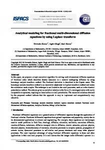
The numerical solutions for the exact solution (3.31) and the approximate solution (3.30) obtained by HATM, for the special case 1 , are shown in Fig. 1 and those for different values of t and α at x = 1 and y = 0.5 are depicted in Fig. 2. It can be seen from the Fig. 1a and b that the solution obtained by the HATM is nearly identical with the exact solution. It is observed from Fig. 1 that u ( x, y, t ) increases with the increase in both x and t. It is also seen from Fig. 2 that as the value of α increase, the displacement u( x, y, t ) increases. It is to be noted that only third order term of the HATM was used in evaluating the approximate solutions for Fig. 1. It is evident that the efficiency of the present method can be dramatically enhanced by computing further terms of u ( x, y, t ) when the HATM is used.
(a)
(b)
Figure 1: The surface shows the solution
(c)
u( x, y, t ) for Eqs. (3.21)–(3.22) when 1 and y 0.5 : (a) Exact
solution (3.31); (b) Approximate solution (3.30); (c) | u ex u app | .
Figure 2: Plots of
u( x, y, t ) vs. t at x = 1 and y= 0.5 for different values of α.
International Scientific Publications and Consulting Services
Communications in Numerical Analysis 2015 No. 1 (2015) 16-29 http://www.ispacs.com/journals/cna/2015/cna-00220/
22
Example 3.2. Next, we consider the following two-dimensional diffusion equation
u 2u 2u 2 2, t x y
0 x 1, 0 y 1, t 0, 0 1,
(3.32)
with the initial condition
u( x, y, 0) e x y .
(3.33)
Applying the Laplace transform on both sides of Eq. (3.32) subject to the initial condition, we have
L[u ]
e x y 1 2u 2u L 2 2 0. s s x y
(3.34)
We define a nonlinear operator as
N [ ( x, y, t; q)] L[ ( x, y, t; q)]
e x y s
1 2 2 L ( x , y , t ; q ) ( x, y, t; q) 0. 2 2 s x y
(3.35)
e x y 1 2 u m1 2 u m1 m (u m1 ) L[u m1 ] (1 m ) L . s s x 2 y 2
(3.36)
and thus
The m th -order deformation equation is given by
L [u m ( x, t ) m u m1 ( x, t )] m (u m1 ).
(3.37)
Applying the inverse Laplace transform, we have
u m ( x, t ) m u m1 ( x, t ) L1[ m (u m1 )].
(3.38)
Solving the Eq. (3.38), for m 1,2,3,..., we get
u 0 ( x, y, t ) e x y , u1 ( x, y, t ) e x y
(2t ) , ( 1)
u 2 ( x, y, t ) (1 )e x y
(2t ) (2t ) 2 2 e x y , ( 1) (2 1)
p 3 : u3 ( x, y, t ) (1 ) 2 e x y
(3.39)
(2t ) (2t ) 2 (2t ) 3 2 2 (1 )e x y 3e x y , ( 1) (2 1) (3 1)
Taking 1, the HATM series solution is (2t ) (2t ) 2 (2t ) 3 (2t ) n u ( x, y, t ) e x y 1 e x y . ( 1 ) ( 2 1 ) ( 3 1 ) ( n 1 ) n 0
(3.40)
International Scientific Publications and Consulting Services
Communications in Numerical Analysis 2015 No. 1 (2015) 16-29 http://www.ispacs.com/journals/cna/2015/cna-00220/
23
Setting α = 1 in (3.32), we reproduce the solution of the problem as follows
(2t ) 2 (2t ) 3 (2t ) 4 u ( x, y, t ) e x y 1 2t e x y 2t . 2! 3! 4!
(3.41)
This solution is equivalent to the exact solution in closed form
u( x, y, t ) e x y 2t .
(3.42)
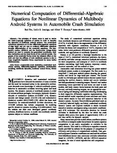
The numerical solutions for the exact solution (3.42) and the approximate solution (3.41) obtained by HATM, for the special case 1 , are shown in Fig. 3 and those for different values of t and α at x = 1 and y = 0.5 are depicted in Fig. 4. It can be seen from the Fig. 3a and b that the solution obtained by the HATM is nearly identical with the exact solution. It is observed from Fig. 3 that u ( x, y, t ) increases with the increase in both x and t. It is also seen from Fig. 4 that as the value of α increase, the displacement u( x, y, t ) increases.
(a)
(b)
Figure 3: The surface shows the solution
(c)
u( x, y, t ) for Eqs. (3.32)–(3.33) when 1 and y 0.5 : (a) Exact
solution (3.42); (b) Approximate solution (3.41); (c) | u ex u app | .
Figure 4: Plots of
u( x, y, t ) vs. y at x = z =1 and y=0.5 and for different values of α.
Example 3.3. Finally, we consider the following three-dimensional diffusion equation
u 2u 2u 2u 2 2 2, t x y z
0 x 1, 0 y 1, 0 z 1, t 0, 0 1,
(3.43)
International Scientific Publications and Consulting Services
Communications in Numerical Analysis 2015 No. 1 (2015) 16-29 http://www.ispacs.com/journals/cna/2015/cna-00220/
24
with the initial condition
u( x, y, z, 0) (1 y)e x z .
(3.44)
Applying the Laplace transform on both sides of Eq. (3.43) subject to the initial condition, we have
(1 y )e x z 1 2u 2u 2u L[u ] L 2 2 2 0. s s x y z
(3.45)
We define a nonlinear operator as
(1 y)e x z N [ ( x, y, z, t; q)] L[ ( x, y, z, t; q)] s
1 2 2 2 L ( x , y , z , t ; q ) ( x , y , z , t ; q ) ( x , y , z , t ; q ) 0. s x 2 y 2 z 2
(3.46)
and thus
(1 y)e x z 1 2 u m1 2 u m1 2 u m1 m (u m1 ) L[u m1 ] (1 m ) L . s s x 2 y 2 z 2
(3.47)
The m th -order deformation equation is given by
L [u m ( x, y, z, t ) m u m1 ( x, y, z, t )] m (u m1 ).
(3.48)
Applying the inverse Laplace transform, we have
u m ( x, y, z, t ) m u m1 ( x, y, z, t ) L1[ m (u m1 )].
(3.49)
Solving the Eq. (3.49), for m 1,2,3,..., we get
u0 ( x, y, z, t ) (1 y)e x z , u1 ( x, y, z, t ) (1 y )e
x z
(2t ) , ( 1)
u 2 ( x, y, z, t ) (1 )(1 y)e x z
(2t ) (2t ) 2 2 (1 y)e x z , ( 1) (2 1)
u 3 ( x, y, z, t ) (1 ) 2 (1 y)e x z 3 (1 y )e x z
(3.50)
(2t ) (2t ) 2 2 2 (1 )(1 y)e x z ( 1) (2 1)
(2t ) 3 , (3 1)
Therefore, the HATM series solution is (2t ) (2t ) 2 (2t ) 3 (2t ) n u ( x, y, z, t ) (1 y)e x z 1 (1 y)e x z . (3.51) n 0 (n 1) ( 1) (2 1) (3 1)
Setting α = 1 in (3.43), we reproduce the solution of the problem as follows
International Scientific Publications and Consulting Services
Communications in Numerical Analysis 2015 No. 1 (2015) 16-29 http://www.ispacs.com/journals/cna/2015/cna-00220/
u ( x, y, z, t ) (1 y)e
x z
25
(2t ) 2 (2t ) 3 (2t ) 4 1 2t (1 y )e x z 2t . 2! 3! 4!
(3.52)
This solution is equivalent to the exact solution in closed form
u( x, y, z, t ) (1 y)e x z 2t .
(3.53)
The numerical solutions for the exact solution (3.53) and the approximate solution (3.52) obtained by HATM, for the special case 1 , are shown in Fig. 5 and those for different values of t and α at x = z =1 and y = 0.5 are depicted in Fig. 6. It can be seen from the Fig. 5a and b that the solution obtained by the HATM is nearly identical with the exact solution. It is observed from Fig. 5 that u ( x, y, t ) increases with the increase in both x and t. It is also seen from Fig. 6 that as the value of α increase, the displacement u( x, y, t ) increases.
(a)
(b)
Figure 5: The surface shows the solution
(c)
u( x, y, z, t ) for Eqs. (3.43)–(3.44) when 1, y 0.5 and z 0.5 :
(a) Exact solution (3.53); (b) Approximate solution (3.52); (c) | u ex u app | .
Figure 6: Plots of
u( x, y, z, t ) vs. y at x = z = 1 and y = 0.5 for different values of α.
International Scientific Publications and Consulting Services
Communications in Numerical Analysis 2015 No. 1 (2015) 16-29 http://www.ispacs.com/journals/cna/2015/cna-00220/
26
4 Concluding remarks In this work, our main concern has been to study the two- and three-dimensional fractional diffusion equations. An approximation to the analytic solution for two- and three-dimensional fractional diffusion equations was obtained by applying the HATM and symbolic calculations. The technique provides the solutions in terms of convergent series with easily computable components in a direct way without using linearization, perturbation or restrictive assumptions. The method is reliable and easy to use. The technique is very powerful and efficient in finding analytical as well as numerical solutions for wide classes of fractional differential equations. In conclusion, the HATM may be considered as a nice refinement in existing numerical techniques and might find the wide applications in science and engineering. Acknowledgement The author is very grateful to the referees for carefully reading the paper and for their comments and suggestions which have improved the paper. The third author is highly grateful to the Department of Mathematics, National Institute of Technology, Jamshedpur, India for the provision of some excellent facilities and research environment. References [1] G. O. Young, Definition of physical consistent damping laws with fractional derivatives, Z. Angew. Math. Mech, 75 (1995) 623-635. http://dx.doi.org/10.1002/zamm.19950750820 [2] R. Hilfer, Applications of Fractional Calculus in Physics, World Scientific Publishing Company, Singapore-New Jersey-Hong Kong, (2000) 87-130. http://dx.doi.org/10.1142/9789812817747_0002 [3] I. Podlubny, Fractional Differential Equations, Academic Press, New York, (1999). [4] F. Mainardi, Y. Luchko, G. Pagnini, The fundamental solution of the space-time fractional diffusion equation, Fractional Calculus and Applied Analysis, 4 (2001) 153-192. [5] L. Debnath, Fractional integrals and fractional differential equations in fluid mechanics, Frac. Calc. Appl. Anal, 6 (2003) 119-155. [6] M. Caputo, Elasticita e Dissipazione, Zani-Chelli, Bologna, (1969). [7] K. S. Miller, B. Ross, An Introduction to the fractional Calculus and Fractional Differential Equations, Wiley, New York, (1993). [8] K. B. Oldham, J. Spanier, The Fractional Calculus Theory and Applications of Differentiation and Integration to Arbitrary Order, Academic Press, New York, (1974). [9] A. A. Kilbas, H. M. Srivastava, J. J. Trujillo, Theory and Applications of Fractional Differential Equations, Elsevier, Amsterdam, (2006). [10] M. Siddique, Numerical computation of two-dimensional diffusion equations with non local boundary conditions, IAENG International Journal of Applied Mathematics, 40 (1) (2010) JAM_40_1_04.
International Scientific Publications and Consulting Services
Communications in Numerical Analysis 2015 No. 1 (2015) 16-29 http://www.ispacs.com/journals/cna/2015/cna-00220/
27
[11] M. Akbarzade, J. Langari, Application of homotopy perturbation method and variational iteration method to three dimensional diffusion problem, International Journal of Mathematical Analysis, 5 (18) (2011) 871-880. [12] A. Cheniguel, Numerical simulation of two-dimensional diffusion equation with non local boundary conditions, International Mathematical Forum, 7 (2012) 2457-2463. [13] S. J. Liao, Beyond Perturbation: Introduction to homotopy analysis method, Chapman and Hall / CRC Press, Boca Raton, (2003). http://dx.doi.org/10.1201/9780203491164 [14] S. J. Liao, On the homotopy analysis method for nonlinear problems, Applied Mathematics and Computation, 147 (2004) 499-513. http://dx.doi.org/10.1016/S0096-3003(02)00790-7 [15] S. J. Liao, A new branch of solutions of boundary-layer flows over an impermeable stretched plate, International Journal of Heat and Mass Transfer, 48 (2005) 2529-2539. http://dx.doi.org/10.1016/j.ijheatmasstransfer.2005.01.005 [16] S. J. Liao, An approximate solution technique not depending on small parameters: a special example, Int. J. Non-Linear Mech, 30 (3) (1995) 371-380. http://dx.doi.org/10.1016/0020-7462(94)00054-E [17] S. J. Liao, A new branch of solutions of boundary-layer flows over an impermeable stretched plane, Int. J. Heat Mass Transfer, 48 (12) (2005) 2529-2539. http://dx.doi.org/10.1016/j.ijheatmasstransfer.2005.01.005 [18] T. Hayat, M. Khan, M. Ayub, On the explicit solutions of an Oldroyd 6-constant fluid, Int. J. Eng. Sci, 42 (2004) 125-135. http://dx.doi.org/10.1016/S0020-7225(03)00281-7 [19] T. Hayat, M. Khan, Homotopy solution for generalized second-grade fluid fast porous plate, Nonlinear Dyn, 4 (2) (2005) 395-405. http://dx.doi.org/10.1007/s11071-005-7346-z [20] A. Shidfar, A. Molabahrami, A weighted algorithm based on the homotopy analysis method: application to inverse heat conduction problems, Communications in Nonlinear Science and Numerical Simulation, 15 (2010) 2908-2915. http://dx.doi.org/10.1016/j.cnsns.2009.11.011 [21] S. Abbasbandy, E. Shivanian, K. Vajravelu, Mathematical properties of h-curve in the frame work of the homotopy analysis method, Commun. Nonlinear Sci. Numer. Simulat, 16 (2011) 4268-4275. http://dx.doi.org/10.1016/j.cnsns.2011.03.031 [22] S. Abbasbandy, Homotopy analysis method for the Kawahara equation, Nonlinear Anal. Real World Application, 11 (2010) 307-312. http://dx.doi.org/10.1016/j.nonrwa.2008.11.005
International Scientific Publications and Consulting Services
Communications in Numerical Analysis 2015 No. 1 (2015) 16-29 http://www.ispacs.com/journals/cna/2015/cna-00220/
28
[23] S. Abbasbandy, Approximate solution for the nonlinear model of diffusion and reaction in Porous catalysts by means of the homotopy analysis method, Chemical Engineering Journal, 136 (2008) 144150. http://dx.doi.org/10.1016/j.cej.2007.03.022 [24] K. Vishal, S. Kumar, S. Das, Application of Homotopy Analysis method for fractional Swift Hohenberg equation- Revisited, Applied Mathematical Modelling, 36 (8) (2012) 3630-637. http://dx.doi.org/10.1016/j.apm.2011.10.001 [25] S. A. Khuri, A Laplace decomposition algorithm applied to a class of nonlinear differential equations, Journal of Applied Mathematics, 1 (2001) 141-155. http://dx.doi.org/10.1155/S1110757X01000183 [26] M. Khan, M. Hussain, Application of Laplace decomposition method on semi-infinite domain, Numerical Algorithms, 56 (2011) 211-218. http://dx.doi.org/10.1007/s11075-010-9382-0 [27] M. Khan, M. A. Gondal, S. Kumar, A new analytical solution procedure for nonlinear integral equations, Mathematical and Computer Modelling, 55 (2012) 1892-1897. http://dx.doi.org/10.1016/j.mcm.2011.11.044 [28] M. A. Gondal, M. Khan, Homotopy perturbation method for nonlinear exponential boundary layer equation using Laplace transformation, He’s polynomials and Pade technology, Int. J. Non. Sci. Numer. Simul, 11 (2010) 1145-1153. [29] S. Kumar, H. Kocak, A. Yildirim, A fractional model of gas dynamics by using Laplace transform, Z. Naturforsch, 67a (2012) 389-396. http://dx.doi.org/10.5560/ZNA.2012-0038 [30] S. Kumar, A Numerical Study for Solution of Time Fractional Nonlinear Shallow-Water Equation in Oceans, Zeitschrift fur Naturforschung A, 68a (2013) 1-7. http://dx.doi.org/10.5560/ZNA.2013-0036 [31] S. Kumar, Numerical Computation of Time-Fractional Equation Arising in Solid State Physics and Circuit theory, Zeitschrift fur Naturforschung, 68a (2013) 1-8. [32] S. Kumar, A new fractional modelling arising in Engineering Sciences and its analytical approximate solution, Alexandria Engineering Journal, 52 (4) (2013) 13-819. http://dx.doi.org/10.1016/j.aej.2013.09.005 [33] S. Kumar, A. Yildirim, Y. Khan, W. Leilei, A fractional model of diffusion equation by using Laplace transform, Science Irantica, 19 (4) (2012) 1117-1123. http://dx.doi.org/10.1016/j.scient.2012.06.016 [34] J. Singh, D. Kumar, S. Kumar, A reliable algorithm for solving discontinued problem arising in nanotechnology, Science Iranica, 20 (3) (2013) 1059-1062.
International Scientific Publications and Consulting Services
Communications in Numerical Analysis 2015 No. 1 (2015) 16-29 http://www.ispacs.com/journals/cna/2015/cna-00220/
29
[35] J. Singh, D. Kumar, S. Kumar, New treatment of fractional Fornberg-Whitham equation via Laplace transform, Ain Sham Engineering Journal, 4 (2013) 557-562. http://dx.doi.org/10.1016/j.asej.2012.11.009 [36] M. Khan, M. A. Gondal, I. Hussain, S. Karimi Vanani, A new comparative study between homotopy analysis transform method and homotopy perturbation transform method on semi-infinite domain, Mathematical and Computer Modelling, 55 (2012) 1143-1150. http://dx.doi.org/10.1016/j.mcm.2011.09.038 [37] D. Kumar, J. Singh, Sushila, Application of homotopy analysis transform method to fractional biological population model, Romanian Reports in Physics, 65 (1) (2013) 63-75. [38] M. M. Khader, S. Kumar, S. Abbasbandy, New homotopy analysis transform method for solving the discontinued problems arising in nanotechnology, Chinese Physics B, 22 (11) (2013). http://dx.doi.org/10.1088/1674-1056/22/11/110201 [39] S. Kumar, D. Kumar, J. Singh, S. Kapoor, New Homotopy Analysis Transform Algorithm to Solve Volterra Integral Equation, Ain Sham Engineering Journal, 5 (1) (2014) 243-246. http://dx.doi.org/10.1016/j.asej.2013.07.004 [40] J. Choi, P. Agarwal, Certain new Pathway type fractional integral inequalities, Honam Mathematical Journal, 36 (2) (2014) 437-447. http://dx.doi.org/10.5831/HMJ.2014.36.2.455 [41] J. Choi, P. Agarwal, Certain Integral Transform and Fractional Integral Formulas for the Generalized Gauss Hypergeometric Functions, Abstract and Applied Analysis, (2014), 2014/ 735946. [42] D. Baleanu, P. Agarwal, On Generalized Fractional Integral Operators and the generalized Gauss hypergeometric Functions, Abstract and Applied Analysis, 2014 (2014), Article ID 630840, 5 pages. http://dx.doi.org/10.1155/2014/630840 [43] H. M. Srivastava, P. Agarwal, Certain fractional integral operators and the generalized incomplete Hypergeometric functions, Abstract and Applied Analysis, 8 (2) (2013) 333-345. [44] P. Agarwal, S. Jain, On unified finite integrals involving a multivariable polynomial and a generalized Mellin Barnes type of contour integral having general argument, National Academy Science Letters, 32 (9-10) (2009) 281-286. [45] F. Mainardi, On the initial value problem for the fractional diffusion-wave equation, in: S. Rionero, T. Ruggeeri (Eds.), Waves and Stability in Continuous Media, World Scientific, Singapore, (1994) 246251.
International Scientific Publications and Consulting Services