IEEE TRANSACTIONS ON MAGNETICS, VOL. 48, NO. 2, FEBRUARY 2012
827
Numerical Computation of Ohmic and Eddy-Current Winding Losses of Converter Transformers Including Higher Harmonics of Load Current Jasmin Smajic1 , Jillian Hughes1 , Thorsten Steinmetz1 , David Pusch1 , Wolfgang Mönig2 , and Martin Carlen3 ABB Corporate Research Ltd., Segelhofstrasse 1K, CH-5405 Baden-Dättwil, Switzerland ABB AG, Keffelkerstrasse 66, D-59929 Brilon, Germany ABB Management Services, Dry-type Transformers, Affolternstrasse 44, 8050 Zurich, Switzerland Two different numerical algorithms for computing the Ohmic and eddy-current winding losses of converter transformers are presented. The higher harmonic components of the nonharmonic electric current, generated by the rectifying part of the power electronic converter, are fully taken into account. The calculated numerical results are verified by comparison with measured results. Index Terms—Converter transformers, eddy-currents, ohmic and eddy-currents winding losses.
I. INTRODUCTION
ARIABLE speed drives are used more and more in industrial production processes, ventilation or pumping systems, and many other applications. The power electronics based converter is able to adjust voltage and frequency which are delivered to the motor, so that its operation is optimized and a minimum of energy is required. The converter consists of a rectifier and an inverter part. The rectifier is fed from the converter transformer. Modern converters contain several rectifier circuits which are fed from different phase shifted coils of the transformer. Converter transformers have therefore more than one secondary winding. An exact knowledge of the losses in a transformer is important for the calculation of its temperature rise and of local hot spots. A fully energized and loaded power transformer dissipates the following electromagnetic losses: 1) hysteresis and eddy-current core losses; 2) Ohmic and eddy-current winding losses; 3) eddy-current structural components losses; 4) Ohmic and eddy-current low-voltage (LV) busbars losses; and 5) Ohmic and eddy-current high-voltage (HV) lead-outs losses [1]. However, the winding losses are the most dominant component, accounting for 60%–80% of the total transformer losses [1]. It is fairly simple to compute the Ohmic winding losses since these losses are caused by the Ohmic resistance of the winding . Having the winding geometry and electric material conductivity of the chosen material (usually either aluminum or copper), it is possible to analytically obtain highly accurate results. On the other hand, the eddy-current winding losses are very difficult to compute. There are several different reasons for that: 1) winding geometry is very complicated; 2) winding geometry contains a large number of small details (thin wires and foils);
V
Manuscript received July 08, 2011; revised September 21, 2011; accepted October 08, 2011. Date of current version January 25, 2012. Corresponding author: J. Smajic (e-mail:
[email protected]). Color versions of one or more of the figures in this paper are available online at http://ieeexplore.ieee.org. Digital Object Identifier 10.1109/TMAG.2011.2171926
and 3) magnetic stray field has a complex spatial distribution that cannot be analytically computed. The first published analytical method for computing the nonuniform current density distribution in the foil-wound transformer winding dates back to 1968 and the work of Mullineux et al. [2]. This analytic approach highly simplifies the problem by introducing several unrealistic assumptions such as: infinitely permeable core, infinite yoke-to-winding distance, and perfectly rectangular windings. Decades later, to overcome these limitations, field computations based on the 2-D finite element method (FEM) were applied as reported in 1998 in the work of Ram [3]. In this paper, the LV winding foils were realistically represented but the HV winding was approximated by stranded blocks. Only the effects of the first harmonic current component (50 Hz) were considered. The increase of the transformer winding losses due to the higher harmonic components of the nonharmonic load current was analyzed and reported for the first time as early as 1970 in the work of Crepaz [4]. It contains an analytical consideration of the increased winding losses due to the nonharmonic rectifier current for two-, six-, and twelve-pulse systems. The outcome of the analysis presented in the work [4] were simple analytical formulas for corrective factors representing the effect of the higher harmonic components. After these initial numerical results, the significance of the problem of increased transformer losses due to the higher harmonic current components was recognized and, consequently, the practice for establishing transformer capability for supplying nonsinusoidal load current was recommended by a sequence of IEC and IEEE standards in [5] and [6]. Compared to the above listed previously published methods and results, this paper contains the following original contributions: 1) two essentially different general algorithms for computing the winding losses of nonsinusoidal load current based on electromagnetic field simulation are presented, 2) both windings (LV and HV) are modeled in their full geometrical complexity and interconnected via direct coupling of the field solver and external electric circuit; and 3) the obtained results of the two methods are verified by comparison against each other and against the measurements. The paper is organized as follows. Section IIdescribes the numerical algorithm for accurately computing the winding losses
0018-9464/$31.00 © 2012 IEEE
828
IEEE TRANSACTIONS ON MAGNETICS, VOL. 48, NO. 2, FEBRUARY 2012
Fig. 2. Geometrical details of the 2-D axisymmetric winding model. Every single wire and foil including the shield for capacitive decoupling of the windings was taken into account.
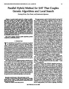
Fig. 1. Winding configuration of the ABB 12-pulse megadrive-LCI [8] (a), its three-phase transformer (b, left), and the mapping of the 3-D real life transformer to its equivalent 2-D axisymmetric model (b, right).
produced by nonharmonic electric current. Section IIIpresents the obtained numerical results, result comparison between the two numerical techniques, and results verification by comparison against the available measurements. Section IVconcludes the paper. II. NUMERICAL ALGORITHMS A typical winding configuration of the rectifier dry-type 11 kV/12 MVA transformer for the ABB 12-pulse megadrive-coad Commuted inverter (LCI) [8] is presented inFig. 1(a). The transformer of this system consists of two LV and one or two HV windings. To achieve the 30 phase-shift required by the 12-pulse rectifier one LV winding is connected to starand the other one to delta-connection. Both HV windings are delta-connected and parallel to each other. The 3-D representation of the rectifier transformer is shown in Fig. 1(b) (left). From the winding losses point of view, it is possible to reduce the 3-D simulation model to its 2-D axisymmetric representation due to evident rotational symmetry of the windings [see Fig. 1(b), right]. This operation involves an error as the yoke and outer limb are not realistically modeled. However, this error is not significant since the stray magnetic field is confined to the air channel between the LV and HV windings marginally affecting the yoke and outer limb. To achieve the level of accuracy required by daily design, the considered 2-D axisymmetric winding model must contain every conductive part of the winding, hence becoming geometrically extremely complex and expensive in terms of CPU
Fig. 3. Nonharmonic load current in time-domain (left) and its harmonic content (right). The current through the delta-connected LV winding and through the star-connected LV winding is depicted in blue and red, respectively.
time and memory requirements. The geometrical details of the chosen winding model are shown in Fig. 2. As one can see, every single turn of the winding was modeled including the very thin shields for capacitive decoupling of the windings. Under nominal operating conditions of the rectifier nonharmonic currents flow through the transformer windings. The measured shapes of these currents and their harmonic contents are presented in Fig. 3. Each harmonic component of the load current causes Ohmic and eddy-current losses in the windings. Therefore, an accurate computation of these losses is of paramount importance for thermal design of such transformers. Different higher harmonic components of the load current have different phase shifts between the delta and star LV winding. Thus, the corresponding higher harmonic stray magnetic fields have spatial distributions very different from the stray fields at 50 Hz and require an accurate field simulation. The first algorithm for computing the winding losses we consider here is based on a 2-D axisymmetric frequency-domain FEM electromagnetic field simulation. For the 2-D axisymmetric quasistatic magnetic analysis in time- and frequency-domain the commercial field solver MagNet of Infolytica was used [7], with the following field formulation implemented (1) (2) (3)
SMAJIC et al.: NUMERICAL COMPUTATION OF OHMIC AND EDDY-CURRENT WINDING LOSSES OF CONVERTER TRANSFORMERS
829
Fig. 4. Equivalent single-phase electric circuit describing the mutual connection of the winding turns and the connection of the windings and current sources.
where is the vector potential, is a scalar electric potential, denotes the magnetic flux density, is the current density, is the angular frequency and is the magnetic permeability. Equation (1) describes the eddy current formulation in the time-domain. The magnetic flux density is derived by (3) and exists in the 2-D x–y plane, whereas the current is orthogonal to that plane. Furthermore, (2) represents the corresponding time-harmonic eddy-current formulation. Having the 2-D axisymmetric model presented in Fig. 2 (left) it is not possible to geometrically define the connections of the windings to each other. Therefore, an electric circuit is needed in order to define these connections. The electric circuit used for modeling of the transformer windings is shown in Fig. 4. A careful study of the nonharmonic load current of the threephase transformer yields the phase shifts of the currents through the LV windings of each coil. Thus, it is accurate enough to model only one phase and use current sources on the LV side as shown in Fig. 4. The first algorithm we applied is based on the harmonic decomposition of the load current (see Fig. 3, right). This algorithm consists of frequency-domain field computations for each harmonic component separately. According to the well-known Parseval’s theorem, the total losses could be obtained as a sum of the separately computed losses for each harmonic component. As an alternative to the first method, the second algorithm is based on the 2-D axisymmetric time-domain field computation coupled with the electric circuit presented in Fig. 2 where the current sources represent the measured nonharmonic currents shown in Fig. 3. Evidently, if performed for a certain number of the load current periods (according to the numerical tests in this case four periods were enough) with a sufficiently small time-step, this algorithm will compute accurate losses in the windings. Evidently, the first frequency-domain approach is less accurate but much faster in terms of CPU time. The second method was used only for verifying the results of the first approach and due to its long CPU time is not so suitable for daily design. III. NUMERICAL RESULTS The obtained stray magnetic fields for the 1st, 5th, 7th, and 11th harmonic component of the load current are shown in Fig. 5. It is very interesting that the spatial field distributions are very similar for the 1st and 11th harmonics. The same level of similarity can be seen between the 5th and 7th harmonics. In the same time, the field distribution of the 1st and 11th harmonic is very different from the field pattern of the 5th and 7th harmonic component. This effect can be explained by the analysis of the phase shift between the delta and star
Fig. 5. Stray magnetic field of the 1st, 5th, 7th, and 11th harmonic component. Evidently the 5th and 7th harmonic component are responsible for producing hot spots due to very high local loss densities in the LV windings close to the separation gap. The given color scale is valid for all the harmonic components but for the 1st harmonic which has the double maximum value (40 000 A/m). More information can be found in the text.
LV windings. This phase shift is equal to 180 for 5th and 7th harmonic yielding the confinement of the stray magnetic field in the gap between the LV coils [see Fig. 5(b)]. On the other hand, this phase shift is equal to 0 for the 1st and 11th harmonic confining the stray field in the cooling channel between the LV and HV coils. This somewhat counter intuitive effect plays a very important role for the thermal design of such rectifier transformers.
830
IEEE TRANSACTIONS ON MAGNETICS, VOL. 48, NO. 2, FEBRUARY 2012
TABLE I RESULTS COMPARISON TRANSIENT COMPUTATION VERSUS HARMONIC SUPERPOSITION
TABLE II RESULTS COMPARISON (50 Hz) FREQUENCY-DOMAIN COMPUTATION VERSUS MEASUREMENTS
The disagreement of the total losses of 6.1% presented in Table IIcan be explained mainly by fabrication tolerances and the accuracy of the measurements. Measurements of the losses with full nonharmonic load are not available at the moment, since this requires a complete installation including converter, motor and a powerful load. Together with previously published algorithms for 3-D computing of the losses in the transformer LV busbars and structural components [9], the presented algorithms for accurate simulation of winding losses are a solid basis for virtual prototyping. This modern design approach radically reduces development time and costs and increases efficiency, quality and reliability of new products. IV. CONCLUSION
Measured data were obtained by performing a routine short-circuit test.
The transformer cooling system should not be designed only according to the usual (50 Hz) distribution of the winding losses. It is also not enough to take into account the total losses based on the addition of the harmonic currents even if they are very accurately estimated or measured on a physical prototype. It is very important to mitigate the problem of eddy-current loss confinement in the region around the air gap between the delta and star LV coils produced mainly by the 5th and 7th current harmonics. The corresponding thermal hot spots could easily cause a local degradation of the insulation which results in a failure and radically reduces the life-time of the transformer. The winding losses computed by using the described transient and harmonic superposition algorithm are compared inTable I. The CPU time of one single field computation in frequency domain was around 30 min. Thus, the total CPU time for computing the losses of the first five dominant harmonic components (see Fig. 3, right) was 2.5 h. The corresponding transient simulation was run for four load current periods (80 ms) with the time-step 0.5 ms. Thus, the total CPU time of the transient simulation was around 3.33 days. Table I shows that the accuracy of the harmonic superposition method is very good which justifies the application of this method in daily design and optimization and allows for radical reduction of the CPU time. Table II shows the comparison of the winding losses computed at 50 Hz against the available measurements. Evidently, a very high level of accuracy is achieved. It is worth mentioning that this level of accuracy is possible to achieve only by having very accurate and measured material property data available. The values of the electric conductivity must be also corrected with respect to the expected operating temperature of the windings.
The effect of higher harmonic components of the nonharmonic load current to the character and distribution of the winding losses of rectifier transformers was investigated. Two different numerical approaches based on time-domain and frequency-domain FEM simulations are presented. The comparison between the obtained numerical results of the two methods reveals a high level of agreement giving advantage to the faster frequency-domain approach. The comparison between the simulation results and measured data shows also a good agreement confirming the reliability of our methods. The presented methods for computing the winding losses together with the previously published methods for simulating electromagnetic losses in core, structural components, and LV busbars [9] constitute a complete set of algorithms for accurate, reliable, and efficient electromagnetic modeling of power, distribution, and rectifier transformers. REFERENCES [1] S. V. Kulkarni and S. A. Khaparde, “Transformer engineering: Design and practice,” in Design and Practice. New York: Marcel Dekker, 2004. [2] N. Mullineux, J. R. Reed, and I. J. Whyte, “Current distribution in sheet- and foil-wound transformers,” in Proc. IEEE, 1969, vol. 116, no. 1, pp. 127–129. [3] B. S. Ram, “Loss and current distribution in foil-windings of transformers,” in Proc. IEEE Gener. Trans. Distrib., 1998, vol. 145, no. 6, pp. 709–716. [4] S. Crepaz, “Eddy-current losses in rectifier transformers,” IEEE Trans. Power App. Syst., vol. 89, no. 7, pp. 1651–1656, Jul. 1970. [5] Converter Transformers—Part 1: Transformers for Industrial Applications, IEC 61378-1, International Electrotechnical Commission, Geneve, Switzerland, 1997. [6] IEEE Recommended Practice for Establishing Liquid-Filled and DryType Power and Distribution Transformer Capability When Supplying Nonsinusiodal Load Current, IEEE Std C57.110-2008, Transformer Committee of the IEEE Power Engineering Society, 2008, IEEE Power Engineering Society. [7] Infolytica MagNet: Design and Analysis Software for Electromagnetics [Online]. Available: www.infolytica.com Infolytica Corporation [8] Medium Voltage AC Drive, MEGADRIVE-LCI for Control and Soft Starting of Large Synchronous Motors, ABB, Switzerland, 2010. [9] J. Smajic, T. Steinmetz, B. Cranganu-Cretu, A. Nogues, R. Murillo, and J. Tepper, “Analysis of near and far stray magnetic fields of dry-type transformers: 3D simulations vs. measurements,” IEEE Trans. Magn., vol. 47, no. 5, pp. 1374–1377, May 2011.