IEEE TRANSACTIONS ON POWER DELIVERY, VOL. 20, NO. 1, JANUARY 2005
71
Computation of High-Frequency and Time Characteristics of Corona Noise on HV Power Line Nermin Suljanovic´, Aljo Mujˇcic´, Matej Zajc, Member, IEEE, and Jurij F. Tasiˇc, Member, IEEE
Abstract—This paper presents an algorithm for the computation of frequency and time characteristics of the corona noise in power-line carrier communications. In the frequency domain, the corona noise is represented with a power spectral density and with a Gaussian noise voltage with variable root mean square value in the time domain. Simulations results are compared with measurements on an actual 400-kV power line. Index Terms—Corona noise, high-frequency power-line modeling, power-line carrier.
I. INTRODUCTION
T
HE QUALITY of digital communications via power lines is determined with the high-frequency power-line model: a power-line transfer function (amplitude and phase frequency characteristic, that is group delay) and a noise behavior. In other words, the power-line high-frequency model will determine boundary conditions for an information transmission via the power line and power-line carrier (PLC) systems design. In PLC communications, the signal is transmitted through the power-line conductors. At the receiver, the transmitted signal is attenuated and corrupted by noise. Since the receiver is connected at line terminals, we are interested in determination of a noise level at these two points. This paper treats an analytic method for estimation of the corona noise appearing at line terminals in frequency and time domain. The corona noise in the frequency domain is described with its power spectrum density while in the time domain it is characterized with a Gaussian noise process of the voltage with time-variable variance. The correlation between frequency and time characteristics of corona noise presented in the paper is based on observations made from measurements on the actual high-voltage (HV) power line and results of the analytic approach. The motivation for corona noise investigation is the fact that the corona is a predominant noise source on the power line in the normal operation. Therefore, a power line appears as a noise source by itself due to corona discharges on HV power lines. Many published papers treat the computation of power loss as well as electromagnetic interference (EMI) caused by the corona in the environment surrounding HV power line. EMI algorithms are also used for the computation of the corona noise level at the line terminals and can be divided in two categories:
Manuscript received June 30, 2003. Paper no. TPWRD-00354-2003. The authors are with the Laboratory for Digital Signal, Image and Video Processing, Faculty of Electrical Engineering, 1000 Ljubljana, Slovenia (e-mail:
[email protected]). Digital Object Identifier 10.1109/TPWRD.2004.838656
empirical and analytic [1], [2]. Analytic EMI algorithms contain two stages. First, determination of corona induced currents that are usually related to an excitation function. The excitation function defines the intensity of the corona on the HV power line and was determined experimentally [3], [4]. The second stage contains the computation of interference electromagnetic fields that are caused by corona induced currents. The proposed algorithm keeps the first stage with exception that instead of excitation function, a generation is used. The relation between the excitation function used in EMI analysis and the generation employed in the corona noise computation for PLC communications is described in the paper. The second stage is a computation of the noise level at line terminals where induced currents due to corona are modeled with shunt current sources. The analytic approach for analysis of the corona induced currents proposed by Adams [3] is based on the electromagnetic theory. This paper introduced a “generating function”, later named the excitation function that is used for representation of a corona current source distributed along the line. Power spectral density of the voltages of power-line conductors is computed from their autocorrelation functions. An alternative approach utilizes a distributed shunt current source representing a corona induced current and computes the currents and voltages propagating along the power line [4]–[7]. Such analysis is conducted in the frequency domain with uniform corona generation. Since the power line represents a multi-conductor system, a modal analysis is used for determination of currents and voltages at arbitrary point of the power line [8], [9]. Conductors coronate over whole line length and total voltages and currents due to all corona sources on the line are obtained with quadratic summation [4], [7]. A. Background When the power line is in operation, a strong electric field exists in the conductor’s vicinity due the rated power frequency voltage. The electric field accelerates free electrons present in the air nearby rated conductor. The directions of electron motion depends on the voltage polarity. These electrons collide with molecules of air, generating a free electron and positive ion couple. This process continues forming an avalanche that is called a corona discharge. Due to positive and negative charges in motion, currents are induced both in the conductors and ground. The induced current appears in the form of current pulse trains, with a random variation of pulse amplitudes and pulse separation intervals [5]. Current pulses propagate toward the both line ends for some distance of the line before they are fully attenuated.
0885-8977/$20.00 © 2005 IEEE
72
IEEE TRANSACTIONS ON POWER DELIVERY, VOL. 20, NO. 1, JANUARY 2005
Fig. 1. Corona on conductor k modeled with shunt current source.
II. COMPUTATION OF POWER-LINE NOISE DUE TO CORONA IN FREQUENCY DOMAIN This section presents the method of corona noise computation for multiconductor line in the frequency domain also presented in [4], [7], [10]. The injected current due to corona on one conductor is modeled with a current source. According to Shockley-Ramo theorem [5], a corona discharge induces currents in all conductors, there is a one current source connected between each conductor and the ground (Fig. 1). The current source in the multiconductor system due to corona on the conductor is usually represented with the vector . The induced current in the conductor due to corona on the conductor is related with the induced current in the conductor with (1) and are the th and th element of the capaciwhere tive coefficient matrix [4], [5], [7], [10]. The noise level is determined for a frequency narrow-band where frequency spectrum of the corona current pulse is considered to be a constant. The computation is done more comfortable if we deal with the sinusoidal process described at the central frequency of frequency band instead with . The magnitude of wide-range process described with should be adopted to provide a power equality of the sinusoidal [4], [7]. and pulse processes in the frequency range The corona current pulse can be modeled as [4] (2) where is a parameter that depends on diameter of conductor [mm] and is found from (3)
Fig. 2. Relative spectrum of corona pulse.
The relative spectrum of corona pulse is presented in Fig. 2 . To obtain the noise level at line terminals caused by corona sources along the whole line length, the first step is determination of a voltage due to one corona source at arbitrary point on the line. The entire noise level is then estimated by quadratic summation of voltages due to all corona sources. The power line is a multiconductor system and provides more than one option for a connection of communication equipment. This is defined by coupling schemes [4], [7]. Different coupling schemes are characterized with different transfer functions since they excite different modes. Coupling the middle phase to ground and the outer phase to inner phase are designated as optimal for the power line with three conductors in horizontal disposition. For the sake of simplicity, we will study the phase to ground coupling and later generalize for the phase to phase coupling. A. Noise Voltage of a Single Corona Source A corona current source connected between the power line and the ground at a random point (Fig. 3) introduces a noise voltage at the same point (5) and correspond to input adwhere square matrices mittances at the point toward the left and right side of the power line. Since all quantities are computed for a given frequency , the argument is omitted in the further expressions. and , When the power line is terminated with admittances matrix reflection coefficients are [4], [7]
The corona current pulse spectrum is further found to be (6) (4)
stands for a power-line characteristic impedance. If where is a propagation function matrix in phase coordinates [4], [8]
´ et al.: COMPUTATION OF HIGH-FREQUENCY AND TIME CHARACTERISTICS OF CORONA NOISE ON HV POWER LINE SULJANOVIC
73
The previous analysis is more comfortably conducted if modal analysis is applied to the previous equations. After employing of the modal analysis [8], (11) becomes (15.1) (15.2) where is the diagonal matrix of modal propagation functions, square complex matrix of transformation from phase to modal coordinates [8] and (16)
Fig. 3. Corona source at point x.
and designates the line length, admittance matrices are computed as [4]
, and
is the characteristic impedance of the power line Matrix in modal coordinates. B. Noise Voltage Due to Power-Line Corona
(7) and are determined with where the matrix coefficients a method of reflection coefficients [4], [7] (8) The voltage at the source connection is related to the voltages at the right and left sides of the line via complex matrices known and as voltage transfer coefficients
The previous section describes the noise level calculation at line ends caused by one corona source. The next step is to obtain a noise level at the line terminals due to all corona sources along the line. The method from [4], [7], and [10] makes an assumption that the noise power at line terminals equals the sum of power generated by all corona sources along the power line. Therefore, it is convenient to compute the square of voltage magnitude at line terminals since it is proportional to the power. Lets consider the phase to ground coupling. If we designate a voltage at the conductor due to the corona source on the , its square can be found as conductor with
(9) The voltage propagation along the left and right line segments (that are considered homogeneous) is affected with the propagation function , the length of line segments while the reflection coefficients incorporate a reflection of voltage waves at the line terminals
(17) The square voltage at the conductor is equal to the sum of square voltages caused by all corona sources on the conductor (18)
(10) Substituting the voltage transfer coefficients in (10) with the expressions defined in (11), we obtain voltages at left and right power-line terminals (11.1)
A simplification of the analysis is made through the assumption that power of the corona sources is uniformly distributed along the line. Then we can replace the sum in (18) with the line integral
(19)
(11.2) where introduced matrices are
(12) (13) (14)
where represents an average distance between two neighbor corona sources on the th conductor. At this point generation ( is used instead of commonly used symbol , which represents the propagation function here) is introduced to avoid a required distance between two neighbor corona sources in the calculation of the corona noise level. Generation characterizes an intensity of corona noise generation. Since high-frequency currents due to corona sources are
74
IEEE TRANSACTIONS ON POWER DELIVERY, VOL. 20, NO. 1, JANUARY 2005
summed as squares, it is comfortable to characterize the intensity of noise with a generation equal to square corona current per unit length in that conductor [4]–[6]
(20) is the rms value of the corona source current in where is the conductor averaged on the length while the generation of conductor . is replaced If the current source in the expression for [a vector whose th element is while with the generation other elements are determined with (1)], the square voltage of the conductor is
C. Generation Versus Excitation Function In the EMI analysis, it is common to use an excitation function instead of generation function. Since there exist many empirical formulae for excitation function, the relation between generation and excitation function is treated in this section. Corona discharges produce pulses of very short duration. These pulses have the same shape but their amplitude and repetition time vary in time around the average value [5], [11]. In the frequency domain, we observe the power spectrum density of one pulse to obtain information how pulse power is in distributed along the frequency axes. The rms value of is the infinitely small frequency interval (25)
(21)
When such pulse passes, the filter without attenuation and with an equivalent bandwidth and a central frequency , the rms value of the signal at the filter output is equal to
From the analysis of noise due to one corona source, the voltage of conductor due to corona source on conductor at arbitrary point is
(26)
(22) and represent the elements in the th row and th while column of the matrices , . The total voltage at the left side of the line due to all corona sources along the line is obtained by introducing previous expression into (21) and integrating in the range from 0 to . Since matrices , , and do not depend on , integration is reduced to exponential terms that are diagonal matrices. After integration, the square voltage of conductor due to corona on conductor at the left power-line terminal is found to be
If is the number of discrete uncorrelated corona sources on the unit length and if denotes the power spectrum density of the th source, the resulting rms value of the filter output caused by all sources on unit length corresponds to excitation function [11]
(27) It is observed that intensity of corona noise generation on the power line is determined by the excitation function. The excitation function is used to represent current pulse trains with the rms value of a corona current at a given frequency averaged over the line’s length. In the EMI analysis, the concept of excitation function is introduced to ensure corona noise computation independently on the power-line geometry [5]. The power-line geometry is incorporated in the propagation analysis of corona pulses. The rms of induced current per unit length in the conductor due to corona on the conductor is [5], [6], [11]
(23) (28) All power-line conductors coronate and square voltage of conductor at the first terminal caused by corona on all conductors is
where is capacitance per unit length of th conductor. Induced current in the conductor is
(24)
(29)
It is not difficult to prove that for the phase to phase coupling analogous equations worth. For instance, if the coupling phase to phase is used instead coefficients and , we use and . coefficients
where is mutual capacitance between conductors and . The (28) and (29) are in accordance with (1). The induced current per unit length and generation are usually expressed in .
´ et al.: COMPUTATION OF HIGH-FREQUENCY AND TIME CHARACTERISTICS OF CORONA NOISE ON HV POWER LINE SULJANOVIC
Comparing (28) with (20), we obtain a relation between generation and excitation function
(30) Different empirical formulae for excitation function that incorporate parameters like a maximum electrical field strength on the conductor’s surface, radius of the conductor and the number of conductors in the bundle are available [1], [4], [12]. However, the corona noise level is also strongly influenced by weather conditions and a state of conductor’s surface. It is observed that noise level deviates at fair weather due to the state of surface of conductors mainly affected by air pollution. On the other hand, the noise level at foul weather (which represents the worst case of corona noise) is more stable and more reliable to predict [12]. D. Determination of Generation From Measured Power Spectrum Density of Noise The corona noise in the frequency domain is characterized with a power spectrum density. If the power spectrum density of the corona noise is measured, the generation can be determined in the following manner. When the conductor of the multiconductor power line coronate, corona currents are induced in all conductors. In accorcan be formed as dance with (1) and (20), vector
75
is the maximal electrical field on the conductor . It where is common to define the generation for the base conductor (for instance, the middle conductor of power line with three conductors in the horizontal disposition) and define generation of other conductors utilizing previous expression. Substituting (33) into (24) with respect to (34), the square voltage on the conductor caused by corona on all conductors of the power line is found to be
(35) Equation (35) states that the voltage on the conductor due to the corona on all conductors is proportional to the generation at a given frequency. Also, we observe that the coefficient of proportionality vary with a frequency. If the power spectrum density of noise at the line terminal is measured, it is more convenient to express the previous equation in terms of power
(36) The power spectrum density of noise is defined in [dBm/Hz]. Therefore, the generation computed in this manner corresponds to the bandwidth 1 Hz [(27)]. If we consider a bandwidth where the power spectrum density can be considered constant, the generation is computed for that bandwidth in accordance with (26) is
(31) (37) Utilizing previous notation for the voltage vector can be rewritten as
, (16) III. TIME CHARACTERISTICS OF CORONA NOISE (32)
and the square voltage of the conductor is
The corona noise on a HV power line is considered as a Gaussian white noise with time-variable rms [4], [7], [13]. Since corona phenomenon is caused by HV, variation of rms of noise will be rather slow and defined with the power frequency interval. The time-variation of the corona noise voltage rms is a periodic function with the period equal to the power frequency period and can be approximately described in one period with three cosine functions [7], [13]
(33) (38) depends only on the powerNote that introduced scalar line geometrical and electric parameters. The corona current induced in the conductor under corona is usually defined in the respect to the base conductor [4]
is , corresponds to the power frequency period where is the Heaviside function. The function in the preand vious expression is
(34)
(39)
76
IEEE TRANSACTIONS ON POWER DELIVERY, VOL. 20, NO. 1, JANUARY 2005
Fig. 5. Principal measuring scheme. Fig. 4. Relative noise voltage.
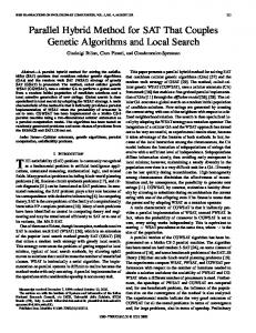
The rms value of the corona noise voltage that corresponds to the value computed in the frequency domain is obtained from the time-variable rms of corona noise as (40) Since the rms value depends on the bandwidth of the filter used in the measuring, instead of (38), it is common to employ the time-variation of rms of the corona noise voltage normalized that appear in the to rms defined with (40). Terms depend on the power line type, relative noise voltage used couplingandweatherconditions.Inaddition,aratiobetween local maximums is also affected by location of intensive corona (heavy raining area). For instance, in the case of the power line with three conductors in the horizontal disposition, outer phase to inner phase coupling, and heavy rain nearby the power-line ter, , minal, the ratios are [4], [7]. The time-variation of corona and noise rms for this case is presented in Fig. 4. IV. MEASURING RESULTS Corona noise voltage in the frequency and time domain was measured on the 400-kV power line with three phase conductors in horizontal disposition. The principal measuring block scheme is given in Fig. 5, while a detailed measuring method and powerline data can be found in [14]. The power spectral density of corona noise is measured with the spectrum analyzer and a result is shown in Fig. 6. The upper curve represents the foul weather noise (corresponds to the relative noise in Fig. 8) while the lower curve is the measurement under fair weather. It can be noticed that noise in foul weather is about 18 dB above the noise at a fair weather. Fig. 6 also presents interference with other PLC devices operating on this and neighboring HV power lines. The relative noise voltage is obtained from measurements acquired with digital oscilloscope Fluke 199 C Scopemeter under different weather conditions. With the aim of presenting the character of the corona noise, this paper contains measure-
Fig. 6. Measured power spectral density of 400-kV power-line noise (upper) foul weather and (lower) fair weather.
ments conducted during foul weather (wet snow on wires) when corona noise is a dominant source of noise on the power line. The time-variable rms of corona noise voltage is computed from the upper envelope of noise voltage waveform recorded with a digital oscilloscope. The oscilloscope is set up to record an envelope, since it is possible to capture a longer data length in this mode. The relative noise voltage computed from the envelope is the same as it computed from the waveform. The recorded data are divided into 20-ms-long blocks, as shown in Fig. 7. If a recorded data block containing elements is divided into 20-ms-long data blocks with elements, the relative noise voltage at the moment is
(41)
´ et al.: COMPUTATION OF HIGH-FREQUENCY AND TIME CHARACTERISTICS OF CORONA NOISE ON HV POWER LINE SULJANOVIC
77
Fig. 9. Algorithm for corona noise estimation.
Fig. 7. Computation of relative noise from recorded data.
Fig. 10. Computed power spectrum density of corona noise (upper) foul weather, (lower) fair weather.
Fig. 8. Computed relative noise voltage from measured data.
where is a sample time. Fig. 8 shows results for total recording time 6 [s] and sample time ( , ) when different filters are used. Each curve in Fig. 9 corresponds to one filter labeled with a filter’s central frequency and equivalent bandwidth expressed in kilohertz. Frequency characteristics of a coupling device and employed filters is provided in the Appendix. The filter labeled with Filt_500 is low-pass filter with cut-off frequency of 500 kHz while other filters are bandpass.
V. SIMULATION RESULTS Computation of the corona noise on the arbitrary HV power line consists of the following.
1) The computation of the power spectral density of corona noise for a given generation. The computation is conducted in the frequency domain utilizing the modal theory. 2) The determination of rms of corona noise voltage from the power spectral density for a selected bandwidth. 3) The corona noise representation as a Gaussian noise with the time-variable rms from computed rms of corona noise voltage and known relative noise. This algorithm is schematically presented in Fig. 9 and is adjusted to steps conducted in this paper. In the case of an arbitrary power line, measured power spectral density and recorded voltage waveform of corona noise used for the determination of generation and the relative noise are skipped. These two quantities are obtained from empiric formulae and recommendations from the literature [2], [7], [12], [13]. The generation is obtained from the measured power spectral density of noise in compliance with algorithm presented in the Section II-C. Eliminating frequencies at which interference occurs, computed average generation for 1-kHz bandwidth is at fair approximately 1.20 at foul weather and 0.16 weather. This generation is used for the computation of power spectral density of corona noise for a 400-kV power line. The result is presented in Fig. 8. Oscillations that appear in the power spectral density of corona noise (Fig. 10) are a consequence of reflection on the power line [4].
78
IEEE TRANSACTIONS ON POWER DELIVERY, VOL. 20, NO. 1, JANUARY 2005
relative noise voltage is computed from the recorded voltage waveforms after different filters. The algorithm for the corona noise estimation is applied to the 400-kV power line with three conductors in horizontal disposition. The measured power spectral density and recorded voltage waveform of corona noise voltage on the 400-kV power line were used for the determination of corona generation and relative noise voltage. We also would like to conclude that the relative noise voltage approximately keeps the shape for different filter bandwidths. This makes opportunity for use of the relative noise as an input parameter in different digital communication techniques for adaptation of their parameters according to time-variations of noise in the channel (like channel coding techniques). APPENDIX Fig. 11. Comparison of rms of power-line noise obtained with computed and measured power spectral density at a foul weather.
The rms of corona noise voltage is obtained from computed power spectral density and known filter characteristics. In the paper, we will take the example of filter with central frequency 273 kHz and bandwidth 34 kHz (Appendix). The computed rms is 177.8 [mV] while measured rms after this filter is 175 [mV]. The time varying corona noise voltage is further obtained from computed rms and relative noise. From Fig. 6, it is obvious that offset should be added to the relative noise defined with (41). Defining that offset is 0.25 and using values from maximums from Fig. 6 for filter 273_34, time-varying power-line noise is computed and presented in Fig. 11. Fig. 11 also presents a comparison of the computed rms of power-line noise with measured. With measured rms is designated the time-varying rms computed from the recorded noise voltage waveform, with the sample time of 2 ms and divided into 120 data blocks. Stars on measurement curve represent actual data while curve itself is obtained with a cubic interpolation. VI. CONCLUSION The boundary conditions for communications via overhead power lines are defined by power-line transfer function and noise characteristics. This paper treats power-line noise due to corona as a dominant noise source on the power line in normal operation. For the purpose of digital communications via power lines, the corona noise is described both in the frequency and time domain. The corona noise is characterized in the frequency domain with the power spectral density of noise while in the time domain it represents the Gaussian noise voltage with time-variable rms. The paper presented the algorithm for corona noise estimation in both frequency and time domain. The algorithm starts with estimation of power spectral density of the corona noise and computation of rms of the corona noise voltage after a filter with an arbitrary transfer function. The rms of the corona noise voltage together with the relative noise is an input for the computation of time-variable rms of the corona noise voltage corresponding to the noise voltage measured after selected filter. The
Fig. A-1. Filter amplitude characteristics. (a) Filter 274_20. (b) Filter 273_34. (c) Filter 280_90. (d) Filter 500.
ACKNOWLEDGMENT The authors are grateful to Iskra Sistemi d.d. for given support and power utility ELES for access to electric power facilities. REFERENCES [1] R. G. Olsen and S. D. Schennum, “A method for calculation wide band electromagnetic interference from power line corona,” IEEE Trans. Power Delivery, vol. 10, no. 3, pp. 1535–1540, Jul. 1995. [2] “Comparison of radio noise prediction methods with CIGRÉ/IEEE survey results,”, IEEE Radio Noise Subcommittee Rep., vol. PAS-92, 1973. [3] G. E. Adams, “The calculation of radio interference level of transmission lines caused by corona discharges,” AIEE Trans., pt. III, pp. 411–419, 1956. [4] G. V. Mikutski, “High-frequency channels on overhead power lines,” in Energy Moscow, Russia, 1986. [5] P. S. Maruvada, Corona Performance on High-Voltage Transmission Lines. Baldock, U.K.: Research Studies Press Ltd., 2000. [6] R. D. Dallaire and P. S. Maruvada, “Analysis of radio interference from short multiconductor lines, part 1,” IEEE Trans. Power App. Syst., vol. PAS-100, no. 4, pp. 2100–2108, 1981.
´ et al.: COMPUTATION OF HIGH-FREQUENCY AND TIME CHARACTERISTICS OF CORONA NOISE ON HV POWER LINE SULJANOVIC
[7] V. H. Ishkin and J. P. Shkarin, Computation of Parameters of High-Frequency Channels on Overhead Power Lines. Moscow, Russia: Power Institute of Moscow, 1999. [8] L. M. Wedepohl, “Application of matrix methods to the solution of traveling-wave phenomena in polyphase systems,” Proc. Inst. Elect. Eng., vol. 110, no. 12, pp. 2200–2212, 1963. [9] N. Suljanovic, A. Mujcic, M. Zajc, and J. F. Tasic, “Power line tap modeling at power-line carrier frequencies with radial-basis function network,” Eng. Intell. Syst., vol. 11, no. 1, pp. 9–17, 2003. [10] J. P. Shkarin, Methodology for computation of high-frequency noise due to corona on power lines, in Electrichestvo, vol. 3, pp. 69–71, 1982. [11] C. H. Gary, “The theory of excitation function: a demonstration of its physical meaning,” IEEE Trans. Power App. Syst., vol. PAS-91, pp. 305–310, 1972. [12] M. R. Moreau and C. H. Gary, “Predetermination of the interference level for high-voltage transmission lines: I—Predetermination of the excitation function,” IEEE Trans. Power App. Syst., vol. PAS-91, pp. 284–291, 1972. [13] Report on Digital Power Line Carrier, CIGRE Study Committee 35, 2000. [14] A. Mujcic, N. Suljanovic, M. Zajc, and J. F. Tasic, “Corona noise on a 400 kV overhead power line: Measurements and computer modeling,” Elect. Eng., vol. 86, no. 2, pp. 61–67, 2004.
Nermin Suljanovic´ received the B.S. and M.S. degrees in electrical engineering from the Faculty of Electrical Engineering, University of Tuzla, Tuzla, Bosnia, in 1997 and 2000, respectively. He is currently pursuing the Ph.D. degree at the University of Ljubljana, Ljubljana, Slovenia. From 1997 to 2001, he was a Teaching Assistant at the University of Tuzla. Since 2001, he has been with the Faculty of Electrical Engineering, University of Ljubljana, engaged in a research project on highspeed digital PLC communications over HV power lines. His research interests are in power line modeling for communication purposes.
79
Aljo Mujˇcic´ received the B.S. degree from the Faculty of Electrical Engineering, University of Belgrade, Belgrade, Yugoslavia, and the M.S. degree from the Faculty of Electrical Engineering, University of Tuzla, Tuzla, Bosnia, in 1992 and 1999, respectively. He is currently pursuing the Ph.D. degree at the University of Ljubljana, Ljubljana, Slovenia. From 1993 to 2001, he was a Teaching Assistant at the University of Tuzla. Since 2001, he has been with the Faculty of Electrical Engineering, University of Ljubljana, engaged in a research project on high-speed digital PLC communications over HV power lines. His research interests include different modulation and channel coding techniques.
Matej Zajc (S’98–A’00) received the B.S. degree from the Faculty of Electrical Engineering, University of Ljubljana, Ljubljana, Slovenia, in 1995, the M.S. degree from the University of Westminster, London, U.K., in 1996, and the Ph.D. degree from the University of Ljubljana in 1999. He is a Teaching Assistant at University of Ljubljana. His research interests include modern communication systems, advanced digital signal processing, and parallel computing.
Jurij F. Tasiˇc (M’86) received the B.S., M.S., and Ph.D. degrees in electrical engineering from the University of Ljubljana, Ljubljana, Slovenia, in 1971, 1973, and 1977, respectively. From 1971 to 1992, he was a Researcher at the Jozef Stefan Institute. Ljubljana. From 1992 to 1993, he was a Visiting Researcher and Professor at the University of Westminster, London, U.K. Since 1994, he has been with the Faculty of Electrical Engineering, University of Ljubljana, where he is currently a Full Professor. His research interests include advanced algorithms in signal and image processing, modern communication systems, and parallel algorithms. Dr. Tasiˇcis a member of EURASIP, the IEEE Slovenian Engineering Society, and the Engineering Academy of Slovenia-IAS. He was the Chair of IEEE Slovenia and is active as a Coordinator and Researcher in COST254, COST276, and other projects.