Numerical Computation of Two-Phase Flow in Porous Media. D. Droste1, F. Lindner1,Ch. ... 2.2 Momentum Conservation. In this model we use Darcy's Law.
Numerical Computation of Two-Phase Flow in Porous Media D. Droste1, F. Lindner1,Ch. Mundt1 and M. Pfitzner1 1 Universität der Bundeswehr, Munich, Bavaria, Germany Abstract: In this study we investigate the heat and mass transfer in a porous media with phase change. The liquid fluid is injected from one side and heated from the other side, where it leaves the porous material in a gaseous state. Dominant forces are capillary interactions and two-phase heat conduction. To model the process we use a two-phase mixture model on a macroscopic scale. This model is presented in two versions. The first version is a one-equation model for energy conservation, while the second is a two-equation model. The versions are implemented in COMSOL and then compared with other results in the literature. A parameter study is done for the second model. Keywords: Two-phase flow, porous media, heat transfer, boiling
1. Introduction In many technical applications two-phase flow with phase change is of importance. In burner with small thermal output the fuel is injected in a liquid state. For an optimal combustion the fuel should leave the porous material in a gaseous state. In other cases such as transpiration cooling, we consider a phase change for cooling processes in porous media. We have to simulate the process of the evaporation to predict the critical heat flux at the surface, at which the fluid is only in a gaseous state. This state known as dryout is an important characteristic for technical design aspects. To simulate these processes, we implement a two-phase mixture model (TPMM), first mentioned by Wang und Beckermann [1], in COMSOL. This model uses the simplification of a local thermal equilibrium (LTE) between the solid matrix and the fluid. Since this oneequation model uses strong assumptions, we also implement an advanced version, which was presented by Shi et al. [2]. This version drops the assumption of the local thermal equilibrium. A qualitative comparison between the two versions is presented. In the first part of this paper, we present the governing equations. The numerical
implementation and the treated problem are described in the following part. The results of the computations and the comparison with results from the literature are done in the next section. In the last part of the paper we give a future prospect.
2. Theory and Governing Equations In this study we consider a homogenous and isotropic porous medium. The one-equation twoPhase Mixture Model is based on the assumption of a local thermal equilibrium (LTE), i.e. the temperature of the solid and fluid phases is the same. The expansion of this version is a twoequation model, which is called the local thermal non-equilibrium model (LTNE). The two versions are only different in the number of energy equations. These models use mixture variables to reduce the number of PDEs. Mixture variables such as mixture density ρ and mixture velocity vector u, are denoted without index. With the help of a diffusive mass flux we can obtain the flow characteristics of the individual phases. 2.1 Conservation of Mass With introduction of the mixture quantities (see [1],[2]) the conservation of mass is defined, with the porosity ε, as 𝜕𝜌 (1) 𝜀 + 𝛻 ⋅ (𝜌𝑢) = 0. 𝜕𝑡 2.2 Momentum Conservation
In this model we use Darcy’s Law 𝐾 (2) 𝑢 = − (𝛻𝑝 − 𝜌𝑘 𝒈) 𝜇 for the momentum conservation. The dynamic viscosity μ and the pressure p are also mixture quantities. 2.3 Diffusive Mass Flux The diffusive mass flux j connects the mixture mean velocity with the velocity of the individual phases. (3) 𝜌𝑙 𝒖𝑙 = 𝜆𝑙 𝜌𝒖 + 𝒋
(4) 𝜌𝑣 𝒖𝑣 = 𝜆𝑣 𝜌𝒖 − 𝒋 Wang and Beckermann introduced the diffusive flux as 𝐾Δ𝜌 𝒋 = 𝐷(𝑠)∇𝑠 + 𝑓(𝑠) 𝒈. (5) 𝜈𝑣 In this definition f is the hindrance function for phase migration and separation and D(s) is the capillary diffusion coefficient as a function of liquid saturation. 2.4 Energy Conservation As we mentioned above, the energy equations are different for the two versions. For the numerical handling, Wang presented a pseudo-mixture enthalpy H. For further details the reader is referred to ref. [3]. First, we present the local thermal equilibrium version. The energy conservation is defined as 𝛻 ⋅ (𝛾ℎ 𝒖𝐻) = ∇ ⋅ (𝛤ℎ ∇𝐻) + 𝐾Δ𝜌ℎ𝑓𝑔 (6) ∇ ⋅ �𝑓 𝒈�, 𝜈𝑣 where hfg is the enthalpy of evaporation, Γh is the effective diffusion coefficient and γh is a corrector coefficient. For detailed information we refer to ref. [3]. Second, the local thermal non-equilibrium version consists of two energy equations. The first equation is similar to equation (6). It is the energy equation of the fluid: 𝛻 ⋅ (𝛾ℎ 𝒖𝐻) = ∇ ⋅ (𝛤ℎ ∇𝐻) + 𝐾Δ𝜌ℎ𝑓𝑔 (7) ∇ ⋅ �𝑓 𝒈� + 𝑞̇ 𝑠𝑓 , 𝜈𝑣 The equation for the solid matrix is the classic conduction of heat equation 𝛻 ⋅ �𝑘𝑠eff ∇𝑇𝑠 � = 𝑞̇ 𝑠𝑓 , (8) where 𝑘𝑠eff is the effective heat conductance. The source term 𝑞̇ 𝑠𝑓 describes the heat transfer between fluid and solid matrix and varies for each domain (liquid, two-phase-domain and gas).
3. Implementation in COMSOL The purpose of this work is to present a useful tool in COMSOL to simulate arbitrary two-phase flows with heat transfer. The introduced model can be implemented in different ways. We used the Darcy’s Law Module and the coefficient form of the PDE Interfaces to implement the rest of the equations.
To validate the implemented model we compare the results with ref. [2] and the analytical temperature at the outlet. This validation is done for the one-dimensional findings. 3.1 Boundary Conditions The principal set-up is shown in figure 1. A continuous mass flux flows against the gravitation from the bottom to the top of the domain. The velocity at the inlet is defined by: 𝑚̇𝑖𝑛 (9) 𝑢𝑖𝑛 = . 𝜌𝑙
Figure 1. Sketch of the one-dimensional problem
The pseudo-mixture enthalpy at the inlet is defined by the inlet-temperature 𝐻(𝑦 = 0) = 𝜌𝑙 �𝑐𝑙 𝑇𝑖𝑛 − 2ℎ𝑣sat �. (10) For the local thermal non-equilibrium version the solid temperature at the inlet corresponds to 𝑇𝑖𝑛 . During the crossing the fluid is heated from the top by a heat source 𝑄̇𝑖𝑛 and starts to boil. The Neumann boundary condition for the enthalpy at exit is given by 𝐾Δ𝜌ℎ𝑓𝑔 d𝐻 (11) (𝑦 = 𝑙) = 𝑄̇𝑖𝑛 − 𝑓 Γℎ 𝑔. d𝑦 𝜈𝑣 In case of the local thermal non-equilibrium version the heat is delivered in the solid material, i.e. 𝑄̇𝑖𝑛 = 0 in equation (11). The boundary condition for the solid energy equation is then defined as d𝑇𝑠 (𝑦 = 𝑙) = 𝑄̇𝑖𝑛 . (12) 𝑘𝑠eff d𝑦 If the heat source is large enough, dryout will be reached. The pressure has the constant value 𝑝𝑜𝑢𝑡 at the outlet.
3.2 Challenges of the Implementation The main challenge of simulating problems with phase change is the jump in the fluid characteristics at the phase transition. Because of the changing characteristics the model is numerical unstable. The effective diffusion coefficient Γℎ , shown in figure 8, degenerates at the phase boundaries, denoted by 𝑠 = 0 (condensation front) and 𝑠 = 1 (evaporation front). To avoid this problem we smoothed the function with the smoothing function of COMSOL. By using a small relative smoothing length, the effect on the result was very slightly (see figure 9).
4. Simulation and results This section is separated in three parts. First, we present the results of the local thermal equilibrium and the local thermal nonequilibrium model and compare the outcomes with each other. Second, we compare the solutions of the local thermal equilibrium model with the results of Shi et al. [2]. Finally, we check the influence of different parameters on the result for the second model. The coolant respectively fuel in our cases is water. The solid material is steel. 4.1 LTE and LTNE The results of the simulations are presented in figure 2, where the temperatures are displayed. The simulation was done for a heating source of 𝑊 𝑄̇𝑖𝑛 = 1.5𝑒6 2 and a mass flux of 𝑚 𝑘𝑔
𝑚̇𝑖𝑛 = 0.5 2 . 𝑚 𝑠 The temperature at the outlet is for each version roughly the same. This is to be expected, because both versions are based on the same theoretical background. We can compute an analytic temperature with the following equation:
𝑇 analytic =
⎧ ⎪
𝑇in +
𝑄̇𝑖𝑛 𝑚̇𝑖𝑛 𝑐𝑙
𝑇sat ⎨ ̇ ̇ ⎪𝑇 + 𝑄𝑖𝑛 − 𝑄Dryout sat ⎩ 𝑚̇𝑖𝑛 𝑐𝑣
if 𝑄̇𝑖𝑛 ≤ 𝑄̇Boil
if 𝑄̇Boil < 𝑄̇𝑖𝑛 ≤ 𝑄̇Dryout if 𝑄̇Dry ≤ 𝑄̇in
The heat constants are defined by (13) 𝑄̇Boil = 𝑚̇𝑖𝑛 𝑐𝑙 (𝑇sat − 𝑇in ) and 𝑄̇Dryout = 𝑄̇Boil + ℎ𝑓𝑔 . (14) However, the distributions are different. The two-phase domain of the local thermal equilibrium is just one third of that from the local thermal non equilibrium version. The reason for this observation is because of the assumption of a thermal equilibrium. This leads to the constant temperature 𝑇sat of the solid and fluid within the two-phase domain, i.e. the heat transfer in the solid matrix is zero. We have an artificial thermal insulation. The local thermal non-equilibrium avoids this problem, by using a second energy equation for the solid material. Thus, temperature gradient for the solid is unequal zero and heat can be conducted in the two-phase region. 4.2 Comparison with Shi Shi et al. [2] use also water as the coolant and steel as the solid matrix. In figure 3 the results of Shi and the results achieved of COMSOL are displayed. These results are computed for different mass fluxes and a heat flux of 𝑄̇𝑖𝑛 = 𝑊 1𝑒6 2 . 𝑚 Our input temperature differs from the input temperature of Shi et al. This difference has no big influence on the results, which we checked for a test case (see figure 10). The results are comparable. The temperature at the outlet is almost the same. And also the qualitative shift of regimes is for both results the same. If we increase the mass influx the temperature at the outlet will decrease and the location of the two-phase domain will be pushed upstream. The main difference in the outcomes is the length of the two-phase domain. The results, computed by Shi, own a longer two-phase region. COMSOL uses the finite element
method, while Shi et al. computes the results with a finite volume method. The results of the COMSOL solver are confirmed by another self-written solver. A finite volume method, implemented in Matlab, delivered the same results in terms of temperature distribution. The discrepancy is not caused by the different solvers. As we mentioned above the different inlet temperature is not the source for the discrepancy. To estimate the quality of the solvers, we compare the temperature at the outlet with the analytical temperature 𝑇analytic 𝑇analytic (15) 𝑟= . 𝑇out The Matlab and COMSOL solver provide the better performance (see table 1). Shi [2] Matlab COMSOL 0,94 0,99 0,99 BC 1 0,98 1 1 BC 2
temperature distributions, the local thermal nonequilibrium is the better choice. In this work we revealed the possibility to implement the two-phase mixture model in COMSOL.
Table 1. Coefficient r (eq. (15))
4.3 Parameter Variation In this section we present two interesting outcomes. First, we show the influence of the coolant on the result and second, the dependence of the relative permeability on the saturation. In figure 4 the results for water respectively ethanol are displayed. Because of the smaller enthalpy of evaporation for ethanol the twophase domain is shorter and the temperature at the exit is much higher. There is a strong connection between the relative permeability krl and the length of the two-phase domain, which we can see in figure 5. Power-law is used for krl(s). The higher the power of the saturation is, the smaller is the twophase domain. A small power pushes the twophase domain upstream.
5. Discussion and future prospect In the previous section we presented the results and saw, that the different models give qualitative the same outcomes. The local thermal equilibrium version delivers roughly the same temperature at the outlet as the local thermal non-equilibrium version. Because of the lower computational cost, this version is good for qualitative analyses. For more realistic
Figure 2. Results of the local thermal equilibrium (LTE) and the local thermal non-equilibrium (LTNE)
5.1 Future Research Points The future work at this topic will concentrate on three points. First, a two-dimensional model will be implemented. In figures 6 and 7 the result of a computation for two dimensions is presented. For this computation, we used large relative smoothing length and gravitational aspects were neglected. The second research point has the aim to drop the assumption of a constant fluid temperature in the two-phase domain. A good approach provides the model of Wei et al. [4]. This model is based on the Gibbs free energy. This energy has to be equal for the liquid and gaseous state within the two-phase domain. Last but not least, we need to verify the model with experimental results.
Figure 5. Results for different relative permeabilities
Figure 3. Comparison between Shi et al. [2] (A) and the COMSOL solver (B) Figure 6. Two-dimensional setting of the problem
Figure 4. Comparison between water and ethanol as coolant Figure 7. Saturation distribution
Figure 8. Diffusion Coefficient with different smoothing degrees
Figure 9. Saturation smoothing degrees
distribution
for
different
Figure 10. Different inlet temperatures
6. References 1. C.Y. Wang and C. Beckermann, A two-phase mixture model of liquid-gas flow and heat transfer in capillary porous media, Int. J. Heat Mass Transfer, Vol. 36, pp. 2747-2758 (1993) 2. J.X. Shi and J.H. Wang, A Numerical Investigation of Transpiration Cooling with Liquid Coolant Phase Change, Transp Porous Med, Vol. 87, pp. 703-716 (2011) 3. C.Y. Wang, A Fixed-Grid Numerical Algorithm for Two-Phase Flow and Heat Transfer in Porous Media, Numerical Heat Transfer, Part B: Fundamentals: An International Journal of Computation and Methodology, 32:1, 85-105 (2007) 4. K. Wei, J. Wang and M. Mao, Model Discussion of Transpiration Cooling with Boiling, Transp Porous Med, (2012)