Oct 23, 2009 - He found a relationship between the differences of arrival time ... immediate neighboring vertex around the considered point which is represented in normal .... reaching the focal points of the beam of light, the triangulation V ...
Numerical estimation of the curvature of a light wavefront in a weak gravitational field A. San Miguel, F. Vicente and J.-F. Pascual-S´anchez Dept. de Matem´atica Aplicada, Facultad de Ciencias.
arXiv:0910.4559v1 [gr-qc] 23 Oct 2009
Universidad de Valladolid, 47005 Valladolid, Spain
Abstract The geometry of a light wavefront evolving in the 3–space associated with a post-Newtonian relativistic spacetime from a flat wavefront is studied numerically by means of the ray tracing method. For a discretization of the bidimensional wavefront the surface fitting technique is used to determine the curvature of this surface at each vertex of the mesh. The relationship between the curvature of a wavefront and the change of the arrival time at different points on the Earth is also numerically discussed.
1
I.
INTRODUCTION
The description of the propagation of light in a gravitational field is even today a central problem in the general theory of relativity. The deflection of light rays and time delays of electromagnetic signals due to the presence of a gravitational field are phenomena detectable with current experimental techniques which allow design new tests for general relativity. In this line, Samuel [1] recently proposed a method for the direct measurement of the curvature of a light wavefront initially flat, curved when light crosses regions where the gravitational field is non vanishing. He found a relationship between the differences of arrival time recorded at four points on the Earth, measured by employing techniques of very long base interferometry and the volume of a parallelepided determined by four points in the curved wavefront surface. This surface is described by means of a polynomial approximation of the eikonal in a Schwarzschild gravitational field. For more complex gravitational models, such as those considered by Klioner and Peip [2], de Felice et al. [3] or Kopeikin and Sch¨afer [4] in studies of light propagation in the solar system, the use of numerical methods for the determination of the geometry of the wavefront surface would also be required. An analytical approach to the relativistic modeling of light propagation has also been developed recently by Le Poncin-Lafitte et al. [5] and Teyssandier and Le Poncin-Lafitte [6], where they present methods based on Synge’s world function and the perturbative series of powers of the Newtonian gravitational constant, to determine the post-Minkowskian expansions of the time transfer functions. Nowadays there are numerous techniques in computational differential geometry which allow to analyze geometric properties of surfaces embedded in the ordinary Euclidean space. Techniques of this type are widely applied in different areas such as Computational Geometry, Computer Vision or Seismology. In one of these methods, developed in works by Garimella and Swartz [7] and Cazals and Pouget [8], the estimation of differential quantities is established using a fitting of the local representation of the surface by means of a height function given by a Taylor polynomial. A survey of methods for the extraction of quadric surfaces from triangular meshes is found in Petitjean [9]. In this work we consider a discretization of the wavefront surface, replacing this surface by a polyhedral whose faces are equilateral triangles. At initial time, the surface is assumed to be flat and far enough from a gravitational source (say, the Sun) and moving towards
2
this source. We study the deformation of the instantaneous polyhedral representing the wavefront when crossing a region in the relativistic 3–space near the Sun due to the bending of light rays by the gravitational field. In this study, we apply the ray tracing method with initial values on the vertices of the triangular mesh to obtain the corresponding discrete surface at each instant of time. Then we apply the techniques given in [7] and [8] to describe the wavefront as a surface embedded in the Riemannian 3–space of the post-Newtonian formalism of general relativity. For each vertex in the instantaneous mesh we obtain a quadric which represents locally the surface by applying the least-squares method to the immediate neighboring vertex around the considered point which is represented in normal coordinates adapted to the light rays. The structure of the paper is as follows: In Section 2 we briefly introduce the basic model for the wavefront propagation in the post-Newtonian formalism. In Section 3, we establish a discretized model of the wavefront surface by means of a regular triangulation and we describe the method employed in this work for the study of the curvature of this surface. In Section 4, a numerical estimation of the curvature of the surface is derived using the ray tracing method. For the numerical integration of the light ray equation, we use the Taylor algorithm implemented by Jorba and Zou [10] which is based on the Taylor series method for the integration of ordinary differential equations and which allow the use of high order numerical integrators and arbitrary arithmetic accuracy, as is required to describe the influence of weak gravitational perturbations on the bending of light rays. Finally, in Section 5, we apply the method discussed above to study the effect of the wavefront curvature on the variation of the arrival time of the light at points on the Earth surface, following the model proposed in Samuel’s test [1]. The paper concludes by giving another approach to the estimation of the curvature of the wavefront, derived from an approximation of the Wald curvature [12] associated with a quadruple of points in the wavefront.
II.
LIGHT PROPAGATION IN A GRAVITATIONAL FIELD
Let us consider a spacetime (M , g) corresponding to a weak gravitational field and choose a coordinate system {(z, ct)} such that the coordinate representation of the metric tensor is gαβ = ηαβ + hαβ ,
with ηαβ = diag (1, 1, 1, −1).
3
(1)
where the coordinate components of the metric deviation hαβ are given by: hab = 2c−2 κkzk−1 δab ,
ha4 = −4c−3 κkzk−1 Z˙ a ,
h44 = 2c−2 κkzk−1
(2)
(Greek indices run from 1 to 4 and Latin indices from 1 to 3) where κ := GM represents the gravitational constant of a monopolar distribution of matter (say the Sun) located at Z a (t) and c represents the light speed. In the post-Newtonian framework one may consider a simultaneity space Σt at each coordinate time t. From the fundamental equation of the geometrical optics for the phase ψ(z, t) of an electromagnetic wave [11]: g αβ
∂ψ ∂ψ = 0, ∂z α ∂z β
(3)
and Cauchy data ψ(z, 0) = const, given on a spacelike surface D0 := {(z, 0) | φ(z) = 0} ⊂ Σ0 one obtains the characteristic hypersurface (light cone) Ω := {(z, t) | ψ(z, t) = const } ⊂ M of the light propagation. The intersection of the characteristic hypersurface and the corresponding simultaneity space is the spacelike wavefront at a time t which will be denoted by St := Ω ∩ Σt . An alternative formulation of the problem of light propagation in the spacetime (M , g) is based on the determination of the bicharacteristics generated by the isotropic vectors � k := grad ψ. From both the equation for the null geodesics, z(t) = z(t), t expressed in terms of the coordinate time and the isotropy condition g(z, ˙ z) ˙ = 0, one obtains in the post-Newtonian approach to general relativity that, neglecting terms of order O(c−2 ), the null geodesics of (M , g) must satisfy the equations ˙ t) z¨a = ϕa (z, z,
(4)
0 = gαβ z˙ α z˙ β .
(5)
˙ t) are given by (see [13]) In (4) the components of the acceleration ϕa (z, z, ˙ t) = ϕa (z, z,
1 2 c h44,a 2
− [ 12 h44,t δka + hak,t + c(h4a,k − h4k,a )]z˙ k −(h44,k δla + hak,l − 12 hkl,a )z˙ k z˙ l −(c−1 h4k,j − 21 c−2 hjk,t )z˙ j z˙ k z˙ a ,
(6)
where the first and third terms in the right hand side of (6) are of order O(1), while the remaining terms are O(c−1 ). 4
For initial values (z 0 , z˙ 0 ), with z 0 ∈ S0 and (z˙ 0 /c, 1), satisfying the condition (5), the integration of the initial value problem corresponding to (4) on an interval [0, T ] allows to determine the spacelike wavefront ST . This surface is embedded in the Riemannian 3–space (ΣT , γ˜ ) where the components of the metric tensor are given by γ˜ab := gab −
ga4 gb4 , g44
(7)
˙ ) to the integral curves z(t) are γ˜ –orthogonal to and at the time T the tangent vectors z(T ST .
III.
NUMERICAL DESCRIPTION OF A SPACELIKE BIDIMENSIONAL WAVE-
FRONT
Hereafter, we consider the simplest gravitational model generated by a static point mass. Let E denote the quotient space of M by the global timelike vector field ∂t associated with the global coordinate system used in the post-Newtonian formalism. We will consider a region of the wavefront in E described by a coordinate chart {z}. Further, we assume that the Riemannian manifold (E , γ ˜ ) is almost flat and that the metric corresponding to γ ˜ is quasi-Cartesian in the chosen coordinates.
A.
Discretization of the initial wavefront
Given an asymptotically Cartesian coordinate system, we consider a set S0 formed by points with coordinates (z1 , z2 , −ζ) where ζ > 0 is a number large enough so that S0 may be considered as a flat surface. The direction determined by the point O∗ : (0, 0, −ζ) in S0 and the center of the Sun O : (0, 0, 0) is perpendicular to S0 . We will study the geometry of a region C ⊂ S0 determined by points P whose Euclidean distances d(P, O∗ ) to the point O∗ satisfy R 6 d(P, O∗ ) 6 2R , where R is the radius of the Sun. For the discretization of the problem we consider, in the first place, the set of points (a1 , a2 , a3 ) ∈ A ∗3 , where A = {0, N1 , N1 +1, . . . , N2 } and N1 < N2 are two natural numbers (see Figure 1(a)). In A ∗3 the point (0, 0, 0) is excluded. Next, we construct in the complex plane a regular triangular mesh whose vertices are located between two hexagons as shown in figure 1(b), and the edges have length `. The inner hexagon has sides of length `N1 and 5
FIG. 1: Triangulation and enumeration of the initial wavefront. (a) Triplets (a1 , a2 , a3 ) ∈ A ∗3 used to label the vertex of a hexagonal mesh V¯. (b) Regular triangulation V ∗ of a hexagonal annular region in the wavefront. Points (3, 4, 0), (0, 3, 4) and (3, 4, 0) in V¯ correspond with points 36, 44 and 50 in V ∗ respectively.
the outer hexagon sides of length `N2 . In this triangulation each vertex is represented by a complex number of the set (see [14]) V¯ := {z = a1 + a2 ω + a3 ω 2 | a1 , a2 , a3 ∈ A , ω := exp(2πi/3)},
(8)
√ −1. The vertices (a1 , a2 , a3 ) with some of their components equal to N1 (resp. N2 ) are located on the inner (resp. outer) boundary of the mesh V¯. We establish an where i :=
enumeration of the vertices as shown in Figure 1(b), in such a way that the inner vertices zj have subscripts j = 1, . . . , J. Finally, we apply the change of scale: V¯ → V ∗ ,
z 7→
zr , N1
(9)
so that the inner boundary is a hexagon of radius r. In consequence the length of each edge in this triangulation is equal to r/N1 . The complex plane and the plane S0 may be identified by means of the mapping ι : z 7→ (