Numerical-Informational Methodology for ...

Numerical-Informational Methodology for Characterising Steel Bolted Components coupling Finite Element Simulations and Soft Computing Techniques

Julio Fernández Ceniceros

A thesis submitted in fulfilment of the requirement for the award of the Degree of Doctor of Engineering

DEPARTMENT OF MECHANICAL ENGINEERING UNIVERSITY OF LA RIOJA

APRIL 2015

I hereby declare that this thesis entitled “Numerical-Informational Methodology for Characterising Steel Bolted Components coupling Finite Element Simulations and Soft Computing Techniques” is the result of my own research except as cited in the references. This thesis has not been accepted for any degree and is not concurrently submitted in candidature of any other degree.

Signature

:

Student

: Julio Fernández Ceniceros

Date

: April 2015

Supervisors : Dr. Francisco Javier Martínez de Pisón Ascacíbar Dr. Andrés Sanz García

Co-Supervisor:

iii

To both Elenas, the past and the future

iv

Acknowledgements

First, I want to express my sincere gratitude to my supervisors Dr. Martínez de Pisón and Dr. Sanz García for their continuous support and encouragement throughout this research. These acknowledgments are extended to the members of the EDMANS research group for their partnership and excellent human approach. The financial support of University of La Rioja through its doctoral fellowship program FPI-UR 2010-14 and grants ATUR 11/16, ATUR 12/11 and ATUR 13/09 are also gratefully acknowledged. Special thanks go to Dipl.-Ing. Volker Diegelmann for kindly hosting my research visit to VDEh-Betriebsforschungsinstitut (BFI). I am also very grateful to Prof. Buick Davison, Prof. Ian Burgess and the rest of the Structural Fire Engineering Research group for their guidance and support during my stay at University of Sheffield. My special gratitude also goes to my family and friends for their constant encouragement. I am deeply indebted to my parents for their trust and the opportunities they have provided me. Last, thank you Satur for your love, patience and unconditional support during this long period. Also thanks to our daughter Elena, who was born in the course of this thesis.

Julio Fernández Ceniceros, Logroño

v

vi

Acknowledgements

Abstract

Over the last few decades, the characterisation of steel joints has been a highly active research topic thanks to its inherent complexity and utmost importance in the behaviour of a whole structure. The emergence of the semi-rigid concept provided significant benefits from both the structural and economic perspectives, in exchange for more advanced and sophisticated calculation procedures. An approach that has gained popularity is the component-based method, in which the overall behaviour of the joint can be determined from the force-displacement responses of its individual components. Although this method is very versatile for modelling any joint configuration, a detailed characterisation of components is necessary to ensure accuracy. In this context, this thesis presents a hybrid methodology to determine the comprehensive force–displacement curve of bolted components: from initial stiffness up to the fracture point. This methodology couples numerical and informational models to predict key parameters of curves, such as initial stiffness, maximum resistance and displacement at failure. To this end, numerical models based on the finite element method (FEM) are first developed to reproduce the real response of bolted components. These models incorporate progressive damage mechanisms and failure criteria to accurately estimate the displacement at fracture. In order to minimise the computational burden of the FEM, the results of a set of simulations are then utilised to train informational models based on soft computing (SC). A genetic algorithm (GA) optimisation is included to set up model parameters and select the most relevant input variables for predicting the force–displacement response. Taken together, the proposed methodology is capable of providing accurate and parsimonious informational models. The applicability of the hybrid methodology is demonstrated for the characterisation of two fundamental bolted components: the lap and the T-stub. The vii

viii

Abstract

results obtained highlight the superior accuracy of this methodology as compared to current regulatory codes and traditional analytical models. Once trained and validated, the informational models are able to replace costly FE simulations without a significant decrease in accuracy, and at a negligible computational cost. Therefore, the hybrid methodology could represent an effective tool to be implemented in structural analysis software for designers and practitioners. Overall, the contributions presented in this thesis provide evidence of the great potential of combining FEM and SC to predict the behaviour of structural components.

Resumen

La caracterización de uniones de acero ha sido un tema de investigación muy activo en las últimas décadas debido a su complejidad y vital importancia en el comportamiento de una estructura. La aparición del concepto semirrígido proporcionó destacados beneficios tanto desde el punto de vista estructural como de la perspectiva económica pero, a su vez, exigió procedimientos de cálculo más sofisticados y avanzados. Un enfoque que ha ganado popularidad entre investigadores y calculistas es el método basado en componentes, capaz de estimar el comportamiento de una unión estructural a partir de las curvas características fuerza-desplazamiento de cada uno de los componentes de la unión. Aunque el método es muy versátil y permite modelar cualquier configuración de unión, es necesaria una detallada caracterización de cada uno de los componentes para conseguir una buena precisión en el cálculo. En este contexto, esta tesis presenta una metodología híbrida para determinar la curva completa fuerza-desplazamiento en componentes atornillados. La metodología combina modelos numéricos y modelos de predicción para estimar parámetros de las curvas, tales como la rigidez inicial, la resistencia máxima o el desplazamiento en la fractura. En primer lugar se desarrollan modelos numéricos basados en el método de los elementos finitos (FEM) para reproducir la respuesta real del componente atornillado. Estos modelos incorporan mecanismos de daño progresivo y criterios de fallo para estimar el desplazamiento en la fractura. Con el objetivo de minimizar el gran coste computacional del FEM, se genera un conjunto de simulaciones para entrenar modelos de predicción basados en soft computing (SC). Estos modelos de predicción incluyen una optimización con algoritmos genéticos (GA) para ajustar los parámetros del modelo y, al mismo tiempo, seleccionar las variables de entrada más importantes en la predicción de la respuesta fuerza-desplazamiento. En su conjunto, la metodología propuesta es capaz de proporcionar modelos de predicción precisos y parsimoniosos. ix

x

Resumen

La aplicación de la metodología híbrida queda demostrada en la caracterización de dos componentes atornillados fundamentales: la unión a solape y la unión en ’T’. Los resultados obtenidos en la caracterización de ambos componentes resaltan la mayor precisión de la metodología propuesta en comparación con las actuales normativas de cálculo y con modelos analíticos tradicionales. Una vez entrenados y validados, los modelos de predicción son capaces de reemplazar a las costosas simulaciones FE sin una pérdida de precisión significativa y con un coste computacional despreciable. Por tanto, la metodología híbrida podría representar una herramienta efectiva para ser implementada en programas de análisis estructural para diseñadores y calculistas. Finalmente, las contribuciones presentadas en estas tesis evidencian el gran potencial de combinar FEM y SC para predecir el comportamiento de componentes estructurales.

Contents

Declaration

iii

Dedication

iv

Acknowledgements

v

Abstract

vii

Resumen

ix

List of Figures

xiv

List of Tables

xv

List of Appendices

xvi xvii

Notation 1 Introduction

1

1.1

Background

1

1.2

Problem statement and motivation of this thesis

5

1.3

Scope of research and objectives

7

1.4

Contributions presented in the thesis

8

1.5

1.4.1

Publications of the thesis

10

1.4.2

Thematic unit

10

Thesis outline

2 Related Works 2.1

10 13

Review of modelling procedures of semi-rigid joints

13

2.1.1

Experimental testing

14

2.1.2

Empirical models

15

2.1.3

Analytical models

18 xi

xii

Contents 2.1.4 Numerical models 2.1.5 Mechanical models Characterisation of basic components in steel bolted connections 2.2.1 Lap component 2.2.2 T-stub component Soft computing techniques applied to steel connections

21 25 33 33 39 47

3 Hybrid numerical-informational methodology 3.1 Numerical model 3.1.1 Contacts definition 3.1.2 Nonlinear constitutive material laws 3.1.3 Failure criteria and progressive damage in structural steel 3.1.4 Solution process: implicit vs. explicit solvers 3.2 Design of computational experiments (DoCE) 3.3 Informational model 3.3.1 Metamodelling techniques

51 53 53 54 56 60 61 62 63

4 PUBLICATION I

67

5 PUBLICATION II

69

6 PUBLICATION III

71

2.2

2.3

7 Results and Discussion 7.1 Characterisation of the lap component 7.1.1 FE model of the lap component 7.1.2 Experimental validation of the FE model 7.1.3 Parametric study 7.1.4 Informational model 7.1.5 Further developments 7.2 Characterisation of the T-stub component 7.3 General discussion

73 74 74 77 81 86 90 97 102

8 Conclusions and Future work

111

Bibliography

115

List of Figures

1.1

Characterisation of the moment–rotation curve

2

2.1

Lap component

33

2.2

Failure modes of the lap component

34

2.3

Different FE approaches for modelling a bolted shear connection (Kim et al., 2007)

36

2.4

Tension zone in steel connections

39

2.5

Failure modes of the T-stub component

40

3.1

Hybrid numerical-informational method

52

3.2

Transformation from nominal to true stress-strain curve

54

3.3

Constitutive material law

56

3.4

Stress-strain curve with progressive damage degradation

58

3.5

Flowchart GA-based optimisation of metamodel training process

64

3.6

Chromosome for the optimisation of setting parameters and input feature selection

65

7.1

FE simulation of bolted lap component

75

7.2

Evolution of the plastic strain and the failure criterion during the loading process

76

7.3

Relationship between plastic strain ratio and stress triaxiality

77

7.4

Experimental validation of test M105

78

7.5

Experimental validation of test B112

78

7.6

Experimental validation of test B114

79

7.7

Comparison of force–displacement responses calculated with implicit and explicit solvers

79

7.8

force–displacement curves for variation of bolt-to-hole clearance

81

7.9

force–displacement curves for variation of plate thickness

82

7.10 force–displacement curves for variation of friction coefficient

83

7.11 Modification of failure mode with variation of friction coefficient

83 xiii

xiv

List of Figures

7.12 7.13 7.14 7.15 7.16

force–displacement curves for variation of yield stress force–displacement curves for variation of ultimate stress force–displacement curves for variation of ultimate strain force–displacement curves for variation of strain at failure Estimation of maximum strength: experimental results (Mõze & Beg, 2010, 2014) vs. theoretical predictions of EC3-1.8 and informational GA-MLPE model 7.17 Characterisation of the force–displacement curve by means of fiveparameter power model 7.18 Graphical comparison of FE simulations and predictions of the informational GA-MLPE model A.1 Comparison experimental-FE model corresponding to the ’M series’ (part 1 of 3) A.2 Comparison experimental-FE model corresponding to the ’M series’ (part 2 of 3) A.3 Comparison experimental-FE model corresponding to the ’M series’ (part 3 of 3) A.4 Comparison experimental-FE model corresponding to the ’B series’ (part 1 of 4) A.5 Comparison experimental-FE model corresponding to the ’B series’ (part 2 of 4) A.6 Comparison experimental-FE model corresponding to the ’B series’ (part 3 of 4) A.7 Comparison experimental-FE model corresponding to the ’B series’ (part 4 of 4) B.1 Evolution of RM SECV and RM SET EST for the prediction of ki B.2 Evolution of RM SECV and RM SET EST for the prediction of kp B.3 Evolution of RM SECV and RM SET EST for the prediction of Fu B.4 Evolution of RM SECV and RM SET EST for the prediction of Ff B.5 Evolution of RM SECV and RM SET EST for the prediction of df B.6 Evolution of RM SECV and RM SET EST for the prediction of n

83 84 85 85

89 92 96

140 141 142 143 144 145 146

of the SC-based metamodel 148 of the SC-based metamodel 148 of the SC-based metamodel 149 of the SC-based metamodel 149 of the SC-based metamodel 150 of the SC-based metamodel 150

List of Tables

7.1 7.2 7.3 7.4 7.5 7.6

Comparison between FE simulations and experimental tests (’M series’ and ’B series’) Comparison between experimental results and theoretical predictions of EC3-1.8 and informational GA-MLPE model DoCE for the prediction of the whole force–displacement curve Results corresponding to test dataset Results of the FS process Input parameters to select six lap components from test dataset

80 90 91 93 94 95

xv

List of Appendices

A Exp. Val. of the FE model of the lap component

139

B Supplementary material for Publication III

147

xvi

Notation

Lower cases b

Width of the T-shape profile

d0

Bolt-hole diameter

dbolt

Nominal bolt diameter

df

Displacement at failure

du

Displacement corresponding to the maximum strength

e1

End distance of the lap component

e2

Edge distance of the lap component

fu

Ultimate stress

fy

Yield stress

h

Number of neurons in the hidden layer

k1

Empirical coefficient for determining the bearing design resistance (Eurocode 3)

ki

Initial stiffness

kp

Post-limit stiffness

m

Momentum xvii

xviii

Notation

n

Number of samples; sharpness parameter; distance from the centre of the bolt hole to the free edge of the flange

pth

Plastic strain threshold at the onset of damage under multi-axial state of stress

q

Gene corresponding to the subset of input features

r

Learning rate; flange-to-web connection radius

s

Gene corresponding to the metamodel setting parameters

tf lange

Flange thickness of the T-shape profile

tinner

Inner plate thickness of the lap component

touter

Outer plate thickness of the lap component

tweb

Web thickness of the T-shape profile

Upper cases A0

Initial cross-section of a specimen

Af

Post-fracture cross-section of a specimen

Anet

Net cross-section

C

Penalty coefficient of support vector machines

D

Damage variable

Dcr

Critical damage

E

Young modulus

Eh

Strain hardening modulus

Eu

Modulus of the true stress–logarithmic strain curve after the strain hardening

F0

Reference force

Numerical-Informational Methodology for Steel Bolted Components Fb,Rd

Design bearing resistance (Eurocode 3)

Ff

Force at failure

Fnet,Rd

Design net-section resistance (Eurocode 3)

Fu

Force corresponding to the maximum strength

G

Generation

J

Fitness function

Lchar

Characteristic length

Lf lange

Flange length of the T-shape profile

Lthread

Thread length of the bolt

P

Population size

R2

Coefficient of determination

S

Metamodel complexity

xix

Greek letters α

Characteristic damage parameter of materials

αb

Empirical coefficient for determining the design bearing resistance (Eurocode 3)

γ

Parameter of radial basis function kernel

γM 2

Partial safety coefficient

ε

Insensitive loss parameter of support vector machines

εf

Strain at failure

εth

Strain threshold at the onset of damage under uniaxial state of stress

xx

Notation

εu

Ultimate strain

εub

Ultimate strain of bolts

εuni,f

Strain at failure under uniaxial stress

λgi

Individual i-th of generation g-th

Λ0

Initial population

µ

Friction coefficient

σm σeq

Stress triaxiality

ν

Poisson’s coefficient

χe

Elitism operator

χm

Mutation operator

Abbreviations 2D

Two-dimensional

3D

Three-dimensional

AN N

Artificial neural network

AU C

Area under the curve

BaggM 5P

Bagging of regression trees (M5P)

BL

Base learner

CDM

Continuum damage mechanics

CI95%

Confidence interval at 95%

CV

Cross validation

DoCE

Design of computational experiments

Numerical-Informational Methodology for Steel Bolted Components

xxi

DS

Direct search

DU CT CRT

Variable associated to the ductile failure criterion (Abaqus)

EC3 − 1.8

Eurocode 3 - Design of steel structures - Part 1-8: Design of joints

EM

Ensemble method

FE

Finite element

F EA

Finite element analysis

F EM

Finite element method

FS

Feature selection

GA

Genetic algorithms

HC

Hard computing

HSS

High strength steel

LHS

Latin hypercube sampling

M 5P

Quinlan’s improved M5 algorithm

M AE

Mean absolute error

M AP E

Mean absolute percentage error

M LP

Multilayer perceptron

M LP E

Multilayer perceptron ensemble

MP O

Model parameters optimisation

MS

Mild steel

NF

Number of features

P EEQ

Equivalent plastic strain (Abaqus)

RF E

Relative fitting error

xxii

Notation

RM SE

Root mean squared error

SC

Soft computing

sd

Standard deviation

SM CS

Stress modified critical strain

SV R

Support vector machine for regression

Chapter 1 Introduction

1.1 Background Steel structures are widely used in the construction of commercial and industrial buildings (Chen & Lui, 2005). They offer great strength/weight ratio, constructability and unalterable properties for the long-term, as opposed to concrete. The design of steel structures primarily consists of determining the member sizes, along with the connections between them. The latter deserve special attention given their essential role in the structural stability of frames. Their main purpose is to assemble the structure and transmit the loads through the structural components. Connections should provide the structure with enough strength to support the loads, as well as ductility so as to allow for slight rotations between beams and columns. The balance between these two characteristics is fundamental not only to resisting monotonic loads, but also to avoiding structural collapse in natural catastrophes, such as seismic loads or fire. Since the terrorist attacks on the twin towers of the World Trade Centre in New York, interest in studying the progressive collapse of steel buildings has been on the rise (Vlassis et al., 2006; Sun et al., 2012). To illustrate the importance of steel connections, let recall that the failure of just one of them could cause the whole building to collapse. A detailed assessment of steel connections is fundamental from both the structural safety point of view and the economic perspective as well. In this regard, steel connections represent about 40% of the total cost of a structure (Díaz Gómez, 2010); hence, an in-depth understanding of their behaviour will 1

2

Chapter 1. Introduction

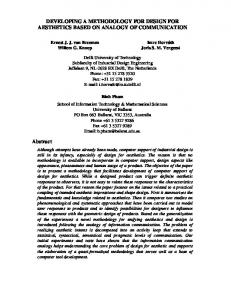
Moment

MRd

ki

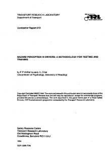
Rotation Figure 1.1: Characterisation of the moment–rotation curve

result in more optimised and lightweight designs and, consequently, remarkable cost savings. In practice, steel connections are either welded or bolted. In general, welding takes place during fabrication, whilst bolting is suitable for on-site connections. Bolted connections have gained popularity due to their ease and speed of erection, and their option of disassembly, as opposed to welded connections. However, although simple to use, bolted connections exhibit a particularly complex behaviour, such that advanced analyses are required to evaluate them (Mohamadishooreh & Mofid, 2008). Since the beginning of last century, the design of beam-to-column bolted connections has attracted the interest of researchers. During this time, the main goal has been the accurate characterisation of joint response, which is defined by the moment–rotation curve (M − Φ). This relationship describes the bending moment applied to the joint M , versus the rotation between connected members Φ. Three main structural parameters define the curve M − Φ (see Figure 1.1): initial stiffness (ki ), moment resistance (MRd ), and rotation capacity (Φ). Originally, connections were ideally classified as nominally pinned or perfectly rigid, regardless of their actual behaviour. This assumption simplifies the calculation procedure to a great degree; however, it could lead to non-conservative results or oversized designs. The actual behaviour of steel joints is generally neither nominally pinned nor perfectly rigid, but rather an intermediate state that endows the joint with rotational stiffness while also allowing a certain degree of rotation between components. Thus, the introduction of the semi-rigid concept promoted the development of new paradigms to assess steel connections. Wilson & Moore (1917) pioneered the study of the rigidity of riveted connections in steel structures. They also conducted experiments on semi-rigid joints and


3

pointed out the inaccuracy of considering connections as perfectly rigid. In the early 1960s, the British Constructional Steelwork Association published the first design procedures for beam-to-column joints in their Black Books (BCSA, 1955; Allwood et al., 1961; Kent & Lazenby, 1964). Later, in 1983, Jones et al. illustrated the need for further research into the effects of semi-rigid connections on structural response. The research project COST Action C1 (1999) merits special attention. It took place during the period between 1991 and 1999, and twenty-three European countries were involved. Its objective was to investigate the behaviour of semirigid joints using different materials (steel, concrete, timber and composites) from both the experimental and analytical perspectives. The impact of this project is patently obvious in 125 individual projects and nearly 400 papers and oral presentations. In the field of semi-rigid steel joints, the research conducted in COST Action C1 served as the basis for the current regulatory code Eurocode 3 Design of steel structures - Part 1-8: Design of joints (European Committee for Standardization (CEN), 2005). Semi-rigid modelling offers several advantages to the structural designer. The use of semi-rigid joints, instead or pinned or rigid ones, modifies the magnitude and distribution of internal forces, as well as the displacements of the connected members (Jaspart, 2000). In pinned joints, the critical moment occurs in the mid-span of the beam, whereas the critical moment in rigid joints is located at the supports. On the other hand, if the semi-rigid approach is adopted, the mid-span moment and the end-moment are balanced and their magnitudes are significantly reduced as compared to pinned and rigid joints. This decrease in the critical moment of beams allows the weight of the connected members to reduce, and thereby produces more economical structures as well. Another benefit of the semi-rigid approach related to pinned joints is the reduction of mid-span deflections. Lastly, the flexibility of semi-rigid joints, as opposed to the rigid model, provides significant potential for supporting seismic loads. Nevertheless, despite the above mentioned economic and structural benefits, this approach still requires a deeper understanding of joint behaviour and the development of more appropriate tools to assess joints. In this regard, this thesis presents an innovative approach that incorporates the capabilities of the finite element method (FEM) and soft computing (SC) techniques to predict the semi-rigid behaviour of steel bolted components.

4


In terms of rotation capacity, steel joints can be classified as ductile, semi-ductile or brittle (Jaspart, 2000). Ductile joints allow an elastic-plastic global analysis to be conducted, whereas brittle ones usually lead to premature failure primarily due to the bolts. From the design perspective, the failure of semi-rigid joints must be ductile to provide enough rotation capacity to form the plastic hinges in the joint (Girão Coelho, 2004). However, the ductility of steel connections is one of the key factors in need of further research. The proper assessment of connection ductility involves not only structural engineering, but also other scientific disciplines to identify and detect failure mechanisms, and to account for progressive damage (Girão Coelho, 2013). In addition to the difficulties of characterising semi-rigid behaviour and ductility, steel connections represent a geometric discontinuity where several components interact (Girão Coelho, 2004). Therefore, the actual behaviour of steel connections is highly nonlinear. The specific phenomena of this nonlinearity are as follows: • Material plasticity: the actual behaviour of steel materials is inherently nonlinear and characterisation beyond the elastic domain is essential for steel components (elastic-plastic properties). • Geometric nonlinearities: characterising, up to collapse, the plastic behaviour of steel joints generally involves large deformations that require nonlinear analysis. • Stress concentration: discontinuities or irregular shapes modify the stress distribution in the vicinity of the irregularity. As a result, peak stress values can be reached locally and cause a crack to start to form. In bolted connections, stress concentration usually takes place in the bolts and in the area surrounding bolt holes. • Contacts: the contact phenomenon between the structural components of the connection is intrinsically nonlinear. When two elements come into contact, the loads are transmitted from one to another by means of normal and frictional forces developed in the interface. The stress distribution in the interface as well as the sticking and sliding conditions are a priori unknown (Girão Coelho, 2004). Thus, dealing with contact phenomena is rather complex and generally requires numerical procedures.


5

The aforementioned nonlinearities and the need to address the semi-rigid concept inspired several methods that characterise the moment–rotation curve, namely: experimental testing, curve fitting, analytical, numerical and mechanical methods. A detailed explanation of each of these methods, their advantages and limitations, as well as the corresponding literature review can be found in Chapter 2 of this thesis.

1.2 Problem statement and motivation of this thesis During the past few decades, researchers all over the world have worked on predicting the real behaviour of steel connections. Different methods have been developed to this end but, in their current states, none of them entirely satisfy the requirements regarding accuracy, versatility and low costs in terms of economy and computational resources. Experimental tests as well as finite element (FE) simulations provide accuracy and reliability in exchange for significant investments of money and time. Therefore, their usefulness as practical design tool is rather limited. Analytical models generally exhibit a strong theoretical background, but the simplifications adopted in their formulae significantly compromise their accuracy. On the other hand, empirical models based on curve-fitting are highly dependent on the tests used to calibrate the models. And consequently, the range of application of this kind of models is very limited. Lastly, mechanical models constitute a general framework applicable to all types of beam-to-column joints. However, their reliability and accuracy relies heavily on the degree of detail characterising the model’s components (Jaspart, 2000). In addition, most existing models focus on determining the initial stiffness and the moment resistance of the joint, while not paying much attention to rotation capacity. This factor, however, is essential to avoiding structural collapse, and takes on even greater importance in the nonlinear behaviour of steel connections subject to extreme conditions, such as seismic loading and elevated temperatures. In short, more accurate and cost-effective strategies are currently needed to model the overall behaviour of steel joints – from initial stiffness up to collapse. It is within this context that the component method (European Committee for Standardization (CEN), 2005), included within mechanical models, offers a framework that is sufficiently general so as to calculate any joint configuration. Moreover, it allows different approaches to be adopted for modelling the nonlinear force–displacement response of each component (Jaspart, 2000; Faella

6


et al., 2000), from simple linear models to much more complex nonlinear curves. It is important to note that a detailed characterisation of components is essential when the nonlinear behaviour of steel joints is required. Many issues concerning this topic remain open to debate. Bolted components constitute highly nonlinear systems where the interactions between bolts and plates produce prying forces, changing sticking-sliding conditions, stress concentrations and bending in bolts, among others. The ductility properties of these components demand special attention since they constitute the sources of deformability in the entire joint. Hence, an adequate assessment of the rotation capacity of joints depends on the level of detail in the characterisation of the ductility of components. This task is extremely complex as it involves not only material plasticity and large deformations, but also progressive damage and fracture.

To date, the characteristic force–displacement response of bolted components has generally been determined by analytical models with a reasonable degree of accuracy (Faella et al., 2000; Piluso et al., 2001a; Jaspart, 1991). These models, however, are not able to account for most local effects present in steel connections, e.g. stress concentrations, sticking-sliding conditions and material degradation. Moreover, bolted components are three-dimensional (3D) in nature, but most analytical models disregard the third dimension. FE models have also been utilised for the simulation of bolted components. In particular, numerous studies have been devoted to characterising the nonlinear behaviour of lap (Chung & Ip, 2000, 2001; Kim et al., 2007) and T-stub components (Bursi & Jaspart, 1997a,b, 1998; Girão Coelho et al., 2006). Despite the ability of these models to deal with the nonlinearities described above, the computational burden of finite element analysis (FEA) renders it impractical for the daily work of structural engineers.

Therefore, an alternative method that would take advantage of FE capabilities at a minimum computational cost is desirable. In this manner, detailed models of bolted components could be efficiently included in the framework of the component method to achieve more accurate results. SC techniques appear to be suitable for this particular task. These techniques have the ability to “learn” from the underlying behaviour of complex problems given a representative input/output dataset. Their use in structural engineering is still rare; however, SC techniques can offer attractive possibilities to tackle the nonlinearities present in steel connections (Fernandez et al., 2010; Diaz et al., 2012).


7

To sum up, the need for an in-depth level of refinement in the characterisation of bolted components, as well as the potential of SC techniques when applied to civil engineering, have impelled the development of this thesis.

1.3 Scope of research and objectives In the framework of the component method, refined modelling of bolted components is of primary importance to assess the entire joint. In particular, the rotation capacity of the joint depends primarily on contributions from individual sources of deformability, i.e. the ductility of bolted components that form the mechanical model. The scope of this research work is, therefore, the development of an innovative approach for predicting the behaviour of bolted components. Special emphasis is placed on the estimation of their constitutive force–displacement laws, from initial stiffness up to failure. The foremost innovation of the method proposed herein is the combination of reliable FEA with advanced SC techniques. Thus, not only can accurate results be obtained, but cost-effective solution times as well. The particular problem addressed in this thesis is the characterisation of two fundamental bolted components: the lap (Mõze & Beg, 2014) and the Tstub (Lemonis & Gantes, 2006). Both components are studied exclusively under monotonic loading conditions; nevertheless, the general method described herein could be extended to other components or even other conditions, such as seismic loading and fire. The following objectives are addressed in this thesis: 1. Development of 3D FE models for the two aforementioned bolted components. The models consider material plasticity, strain hardening and failure criteria based on progressive damage, so as to characterise the ductile behaviour of bolts and plates. 2. Validation of the FE models with experimental tests. 3. Generation of representative datasets that relate the geometry and mechanical properties of bolted components with key parameters of their corresponding force–displacement curves. Design of computational experiments (DoCE) is conducted for this purpose.

8

Chapter 1. Introduction 4. Training and validation of informational models based on SC techniques. Feature selection, complexity metrics and optimisation of model parameters are taken into account in order to achieve not only accurate models, but also generalisation capability. 5. Representation of comprehensive force–displacement curves of bolted components, and comparative studies with regulatory codes and analytical models available in the literature.

1.4 Contributions presented in the thesis The research conducted for this thesis has contributed three scientific publications: Publication I (Fernandez-Ceniceros et al., 2015a). The article aims to characterise the lap component using a numerical-informational approach. The numerical model includes a failure criterion based on continuum damage mechanics (CDM) to detect crack initiation and, consequently, to estimate the ductility of the bolted component. As a result, the FE model is able to accurately simulate the whole force– displacement response and also identify the components’ failure modes. After that, a DoCE is created in order to generate a representative dataset for the subsequent training process. The output information of the DoCE is obtained from the FE model. Lastly, concerning the informational model, the article introduces an ensemble based on multilayer perceptron (MLP) neural networks. It also implements feature selection (FS) and model parameters optimisation (MPO) within a genetic algorithms (GA) scheme. The proposed informational model clearly outperformed single MLPs and other techniques such as support vector machine for regression (SVR) and regression trees. The numerical model and the DoCE were created, planned and implemented by the author of this thesis. Sanz-Garcia took part in the implementation of the ensemble model and also in the interpretation of the results. The majority of the article was written by the author of this thesis. Publication II (Fernandez-Ceniceros et al., 2015b). This article constitutes the first part of a numerical-informational method for characterising the ductile behaviour of the T-stub component. The prin-


9

cipal objective of the study is to develop an advanced FE model capable of obtaining the complete force–displacement curve, including the softening branch. To this end, the FE model considers nonlinear continuum damage mechanisms to simulate the onset of the damage, the damage evolution law and the failure of the component. The reliability of the numerical model was verified with the experimental results of 18 tests. The ratios between experimental and numerical results indicate a satisfactory agreement in the estimation of initial stiffness, maximum strength and the ultimate displacement of the T-stub. However, the main limitation of the proposed model is its high computational cost involved not only in the simulation process, but also in the pre-processing and post-processing tasks. The companion paper (herein referred to as Publication III) addresses this significant limitation. The author of this thesis was responsible for the implementation of the numerical model. He also planned the experimental validation which was carried out at the University of La Rioja with the help of the rest of the co-authors of this study. The article was written entirely by the author of this thesis.

Publication III (Fernandez-Ceniceros et al., 2015c). Taking advantage of the FE model developed in the companion paper, the second part of this contribution presents an informational model to predict the key parameters of the force–displacement curve. To this end, SVR models were trained and tested from representative datasets generated via FE simulations. One of the main novelties introduced in this publication is related to the training process. A GA scheme similar to that utilised in Publication I is employed to achieve a twofold objective: improve the accuracy of metamodels and obtain parsimonious metamodels with high generalisation capacity. For this purpose, the metamodel selection process includes a complexity criterion based on the combination of the number of features and support vectors. This criterion prioritises those metamodel configurations with similar accuracy and lower complexity. The DoCE as well as the interpretation and discussion of the results was planned and carried out by the author of this thesis. Martínezde-Pisón provided insight into the GA-SVR basis and assisted signi-

10

Chapter 1. Introduction ficantly in obtaining a workable implementation of the informational model. The article was written entirely by the author of this thesis.

1.4.1 Publications of the thesis The content of this thesis includes three peer-reviewed scientific articles published in journals listed in the Journal Citation Reports®: 1. Fernández-Ceniceros, J., Antoñanzas-Torres, F., Martinez-de-Pison, F.J. & Sanz-Garcia, A. (2015). Hybrid modelling of multilayer perceptron ensembles for predicting the response of bolted lap joints, Logic Journal of the IGPL. DOI 10.1093/jigpal/jzv007 2. Fernández-Ceniceros, J., Sanz-Garcia, A., Antoñanzas-Torres, F. & Martinezde-Pison, F.J. (2015). A numerical-informational approach for characterising the ductile behaviour of the T-stub component. Part 1: Refined finite element model and test validation, Engineering Structures 82(15), 236-48. 3. Fernández-Ceniceros, J., Sanz-Garcia, A., Antoñanzas-Torres, F. & Martinezde-Pison, F.J. (2015). A numerical-informational approach for characterising the ductile behaviour of the T-stub component. Part 2: Parsimonious soft-computing-based metamodel, Engineering Structures 82(15), 249-60.

1.4.2 Thematic unit The overall context surrounding the publications informing this thesis is the study of steel bolted components, within the framework of the component method. The common denominator of the three articles included herein is a comprehensive numerical-informational method based on coupling FE simulations with SC techniques. Hence, in addition to the fields of civil and structural engineering that address the behaviour of steel connections, the present study also involves two other areas: FEA and predictive modelling.

1.5 Thesis outline This dissertation is organised in eight chapters. The present chapter briefly introduces the topic of steel connections. This section also explains the motivation of this thesis, as well as its scope and objectives. Chapter 2 references previous studies on the assessment of bolted connections, with a special emphasis on the


11

lap and T-stub components. The state-of-the-art of SC techniques applied to steel connections is also addressed in Chapter 2. Chapter 3 is devoted to the numericalinformational methodology that constitutes the core of this research. Chapters 4 through 6 contain the scientific publications contributing to this thesis. The first of these publications focuses on modelling the lap component, whereas the other two deal with the nonlinear behaviour of the T-stub component. Chapter 7 summarises the most remarkable results and also presents a general discussion. Finally, Chapter 8 draws the conclusions of this thesis and suggests new lines of future research.

12


Chapter 2

Related Works

The literature review presented in this chapter is divided into three sections. Firstly, a review of the most remarkable works is presented in order to set the stage for the existing methods characterising steel connections. In the second section, the focus shifts to the two bolted components that constitute the core of this thesis: the lap and the T-stub. Both analytical and numerical approaches are reviewed in this section. Lastly, the third section presents an overview of the SC techniques applied in behaviour characterisation of steel connections.

2.1 Review of modelling procedures of semi-rigid joints For many years, the design of steel joints was conducted in isolation from the design of structural members (Colson et al., 1999). Steel joints were designed as nominally pinned or perfectly rigid immediately after calculating the sizes of beams and columns. Therefore, there was no interaction between the joints and the connected members. The appearance of the semi-rigid concept allowed joint design to be integrated into the global frame analysis. However, this new assumption required comprehensive modelling of the moment–rotation curve. The complexity inherent in accurately assessing this curve is largely due to the massive amount of input variables influencing the characteristic response of the semi-rigid joint. Thus, the complex task of modelling the behaviour of semi-rigid joints has been addressed from various perspectives. 13

14

Chapter 2. Related Works

2.1.1 Experimental testing Numerous experimental tests have been conducted over the last few decades and some authors have compiled them in databanks. These collections of tests contain several types of beam-to-column connections and supply the geometry and material properties for each connection as well as its characteristic moment–rotation response. The first databank was developed by Goverdhan (1983) and consists of tests conducted in the USA between 1950 and 1983. The joint typologies included in this databank are double web angle connections, single web angle/plate connections, header plate connections, end-plate connections and top and seat angle connections. On the other hand, Nethercot published the first European databank in 1985 (Nethercot, 1985a,b). This study comprises over 700 tests for the period between 1915 and 1985, and includes the T-stub connection with and without web angles, in addition to the typologies examined by the Goverdhan databank. Following the work commenced by Goverdhan, Kishi and Chen examined experimental tests conducted all over the world from 1936 to 1986 (Kishi & Chen, 1986b,a). They also created a computerized database, the Steel Connection Data Bank (SCDB) program (Chen & Kishi, 1989; Chen & Toma, 1994; Abdalla & Chen, 1995), to systematically control the databank by means of tabulating and plotting functions. More recently, Kishi and Chen (2010) updated their databank which currently contains a total number of 486 experimental tests from 1936 to 2010. Lastly, SERICON (Weynand et al., 1998) and SERICON II (Cruz et al., 1998) are databanks developed within the COST Action C1 project and include European experimental tests from both steel and composite connections. Without a doubt, experimental testing represents the most accurate method to obtain the moment–rotation curves of semi-rigid joints. However, this approach is very expensive and inappropriate for the daily design work of structural engineers. Nowadays, experimental tests are performed purely for research purposes. Specifically, they are used to validate other kinds of modelling methods, such as analytical and FE models. On a similar note, the usefulness of steel connection databanks lies exclusively in validating the methods proposed by the scientific community. In fact, from the structural designer’s point of view, it is highly unlikely one would find a specific design in the databank due to the vast number of joint configurations and geometrical parameters.


15

2.1.2 Empirical models Empirical models represent mathematical expressions fitted to moment–rotation curves, which are usually obtained from experimental data. These models are able to closely fit the connection response to the tests by calibrating a set of parameters. In general, these parameters are related to the geometry and material properties of the steel joint. However, they usually lack physical meaning because the procedure used to obtain them is based on regression analysis. As a result, it is not usually possible to determine the influence of each joint feature on the overall response of the joint (Diaz et al., 2011a). Moreover, the range of application of empirical models is limited to the joint configurations used for fitting the mathematical expression. Therefore, their reliability and applicability are strongly dependent on the number of experimental tests available to calibrate the empirical model. The first attempt to fit experimental tests to mathematical expressions was carried out by Batho & Lash (1936). They used a simple form of the power function that relates the applied bending moment and the joint rotation: M = C·θ0.412

(2.1)

where C is a constant that depends on the type and dimension of the structural joint. An inverse version of this power function was used by Krishnamurthy et al. (1979) to assess the rotational behaviour of end-plate connections. Krishnamurthy conducted a broad parametric study of 168 connections and 559 loading conditions by means of a two-dimensional (2D) finite element model. This numerical model had been previously validated against thirteen experimental tests on end-plate connections (Krishnamurthy & Graddy, 1976). Finally, the parameters that define the empirical model were derived by regression analysis from the results of the parametric study. Thus, the nonlinear moment–rotation curve of extended end-plate connections can be obtained as follows: θ = C·M α

(2.2)

where α = 1.58 and C depends on the geometry and material properties of beam and connection. It is important to note that the above model is independent of the column properties. Therefore, the assessment of the moment–rotation curve refers to the connection alone rather than the whole joint. Following the same method proposed by Krishnamurthy, Kukreti et al. (1987) conducted a FE parametric study of flush end-plate connections and ob-

16


tained an empirical model from the results of the parametric study. In (Kukreti et al., 1990), they also applied this same method to extended end-plate connections with eight bolts in the tension zone. The introduction of three- and four-parameter power models allowed for more control over the fundamental properties of the moment–rotation curve. Regarding three-parameter power models, Kishi & Chen (1990) developed an equation that relates the moment–rotation curve with the initial stiffness (ki ), the ultimate moment capacity (Mu ), and a shape factor (n): ki ·θ M=h n i 1 n i ·θ 1 + kM u

(2.3)

This expression (Eq. (2.3)) was employed to assess semi-rigid connections with angles (Kishi & Chen, 1990). Furthermore, Ang & Morris (1984) were the first to use a standardised version of the three-parameter Ramberg-Osgood relationship (Ramberg & Osgood, 1943). This mathematical expression, similar to Eq. (2.3), depends on the initial stiffness (ki ), a reference bending moment (M0 ), and a shape parameter (n), according to Eq. (2.4): "

θ M M = 1+ θ0 M0 M0

n−1 #

(2.4)

being: M0 = ki ·θ0

(2.5)

Years later, Abolmaali et al. (2005) also used the Ramberg-Osgood relationship (Eq. (2.4)) and the three-parameter power model (Eq. (2.3)) to assess flush end-plate connections. In this case, they first developed a FE model verified with the experimental tests performed by Srouji et al. (1983). The FE model was run through a test matrix with 34 specimens by varying the geometry of the connection. Finally, the moment–rotation curves obtained numerically were fitted to both the Ramberg-Osgood and the three-parameter power equations. The main limitations of this model were, on one hand, the relatively low number of specimens (34) used to fit the equations and, on the other hand, the lack of material properties in the proposed formulation. Concerning four-parameter power models, Attiogbe & Morris (1991) introduced empirical expressions for the characterisation of double web angle con-


17

nections. Specifically, they used a nonlinear representation based on the Goldberg and Richard relationship (Goldberg & Richard, 1963; Richard & Abbott, 1975), as follows: (ki − kp ) θ (2.6) M= 1 + kp ·θ −kp )θ n n 1 + (kiM 0 where ki and kp are the initial and the post-limit stiffness respectively; M0 refers to a reference bending moment and n represents the sharpness of the curve. These parameters were derived by regression analysis from experimental data and they are exclusively related to the geometry of the joint. One of the main advantages of the four-parameter power model, compared to the Ramberg-Osgood representation, is its ability to deal with positive, zero and negative values of kp . Another approach to the development of empirical models consists of fitting moment–rotation curves to polynomial functions. Sommer (1969) was the first to fit polynomial series to assess welded header plate connections. However, the most popular polynomial model was developed by Frye & Morris (1975) according to the following expression: θ = C1 (K·M ) + C2 (K·M )3 + C3 (K·M )5

(2.7)

where K depends on the geometrical and material properties of the structural joint and C1 , C2 , C3 are curve-fitting constants derived by the least square method. The authors calibrated the constants with 145 experimental tests and for seven typologies of steel connections, ranging from the most flexible singleweb angle connection to the stiffest T-stub connection. The main disadvantage of the Frye and Morris model is that its first derivative, which corresponds to the rotational stiffness, can adopt either positive or negative values. From the structural point of view, negative values of rotational stiffness are completely unrealistic. In this regard, Azizinamini et al. (1985) proposed a modification of the K parameter in order to avoid the numerical difficulties of the previous model. As an alternative to the aforementioned power models and polynomial series, exponential functions are also employed to fit moment–rotation curves to experimental data. In 1986, Lui & Chen proposed a multi-parameter exponential model: !# " m X |θ| + M0 + Rkf |θ| (2.8) M= Cj 1 − exp − 2jα j=1 where M0 represents the initial connection moment, Rkf is the strain hardening connection stiffness, α is a scaling factor for numerical stability, and Cj refers to the j-th curve-fitting parameter obtained from a linear regression analysis.

18


Despite the excellent fit of this model, it is not capable of properly capturing abrupt changes in the slope of the curve. Kishi & Chen (1986b) updated the exponential model proposed by Lui and Chen to accommodate linear components of the moment–rotation curve (Eq. (2.9)): M = M0 +

m X j=1

"

Cj

|θ| 1 − exp − 2jα

!#

+

n X

Dk (|θ| − |θk |) ·H [|θ| − |θk |] (2.9)

k=1

where Dk refers to the k-th curve-fitting parameter for the linear region of the curve, θk is the starting rotation of the k-th component of the curve and H [θ] is the Heaviside’s step function (1 for θ ≥ 0 and 0 for θ < 0). The literature includes other types of mathematical expressions for fitting empirical models. A cubic B-spline model was proposed by Jones et al. (1980) to fit moment–rotation curves to experimental tests. While very accurate, this approach required a large amount of data for calibration. Furthermore, Lee & Moon (2002) created a two-parameter logarithmic model to describe the behaviour of semi-rigid connections with angles, according to the following expression (Eq. (2.10)): h in M = α· ln 103 nθ + 1 (2.10) where α and n are shape parameters derived by the least mean square method with experimental tests. This logarithmic model can be considered semi-analytical because the empirical parameters α and n are directly related to analytical expressions of ki and kp . More recently, Brunesi et al. (2014) developed a closed-form expression for the prediction of initial stiffness in top- and seat-angles and double flange angle connections. Firstly, a parametric study based on a 3D FE model was conducted. Then, the closed-form expression was calibrated by a linear fitting procedure with the data previously obtained in the parametric study. As a result, the closedform expression depends solely on the geometry of the bolts and components and provides a time-saving tool for early design purposes.

2.1.3 Analytical models The primary aim of analytical models consists of calculating the fundamental parameters of the moment–rotation curve separately, i.e. initial stiffness, moment resistance and rotation capacity. For this purpose, analytical models apply


19

the basic concepts of structural analysis (equilibrium, compatibility and material constitutive laws (Del Savio et al., 2009)) to relate the moment–rotation parameters with the geometry and mechanical properties of steel connections. The analysis process is as follows: firstly, the deformation sources and the collapse mechanisms of the connection are identified. Secondly, a simplified model based on elastic analysis is adopted to predict the initial stiffness of the connection. Additionally, plastic mechanisms are modelled to estimate the connection’s moment resistance. And lastly, mathematical expressions are used to generate the moment–rotation curve. In 1934 Baker was the first to attempt to model the moment–rotation curve by means of analytical expressions, followed by Rathbun in 1936. Both of them assumed joint behaviour to be linearly elastic and thus, the overall moment– rotation response was modelled exclusively with the initial stiffness (Eq. (2.11)): Z=

θ M

(2.11)

where Z represents the initial tangent flexibility, which is the inverse of the initial stiffness ki . This linearly elastic assumption was included in early methods of frame analysis with semi-rigid joints. However, the elastic assumption became notably inaccurate for high values of plastic joint rotation. To overcome this problem, bilinear (Melchers & Kaur, 1982; Lui & Chen, 1983), trilinear (Moncarz & Gerstle, 1981) and even multi-linear (Poggi & Zandonini, 1985; Del Savio et al., 2009) models were proposed to predict the moment–rotation curve as dependent on initial stiffness, moment resistance and other related parameters such as yielding moment, plastic moment and post-limit stiffness. The most detailed representation of the moment–rotation curve is obtained by means of nonlinear mathematical expressions. In addition to the key properties of the moment–rotation curve, these mathematical expressions also include a sharpness parameter that should be calibrated empirically with experimental data. Thus, this kind of model can be considered a semi-analytical model. However, analytical models clearly differ from empirical ones in how they predict the key properties of the moment–rotation curve. Extensive literature is available regarding analytical models fitted by nonlinear mathematical expressions. In 1986, Yee & Melchers presented the analytical formulae of a four-parameter model for the assessment of end-plate eave connections. In this study, the authors first identified the possible failure modes in order to calculate the moment capacity of the joint. They also determined that

20


the ultimate moment was governed by the weakest connection component and its value could be obtained from the strength of that component. The rotational stiffness was obtained from the contributions of the connection components to joint deformation. Similarly, analytical expressions were derived for the calculation of post-limit stiffness. Finally, the sharpness parameter of the nonlinear moment–rotation curve was obtained empirically from test results. The foremost advantage of the model proposed by Yee and Melchers is that three of its four model parameters can be determined exclusively by joint geometry.

Kishi and Chen achieved remarkable advances in the characterisation of semi-rigid connections with angles (Kishi & Chen, 1990). They focused on the development of analytical formulae to predict the initial stiffness and the moment capacity of single and double web-angle connections as well as top- and seat-angle connections. Several simplifications were adopted to handle the complex behaviour of angles and their interactions with beams and columns. As a result, the authors developed simple-to-use equations suitable for hand-calculation. They used a three-parameter power model for the nonlinear characterisation of the moment–rotation curve. This power model required a shape parameter that was initially obtained by a least square curve fitting with experimental tests (Kishi & Chen, 1986b). To overcome this dependence on experimental data, the authors proposed logarithmic expressions (Kishi et al., 1991) to estimate the sharpness of the moment–rotation curve. Finally, in order to supply a practical procedure for the design of semi-rigid connections with angles, Kishi et al. (1993) developed a set of nomographs to provide the structural engineer with a direct way to determine the values of initial stiffness, moment capacity and shape parameter. In addition, the non-dimensional form of analytical equations provided the influence of the geometrical parameters on the complex behaviour of connections with angles.

The characterisation of the moment–rotation curve by means of analytical expressions is still widely used among researchers. In 2009, Pirmoz et al. described a semi-analytical model for the assessment of bolted top-seat angle connections. Starting with an analytical model of the connection, they obtained modification factors based on nonlinear FE simulations to consider effects that were not included in the original model. The proposed semi-analytical model was able to account for the influence of material strain hardening and the effects of axial loads.


21

More recently, Yang & Tan (2013) presented a mechanical model which includes analytical expressions for the deformation capacity of angle connections. The innovative aspect of this model is that it takes into account the interaction between angles and bolts, the inclusion of failure criteria to estimate the deformation capacity, and the bolt fracture. Other recent research in the development of analytical models has been done by Loureiro et al. (2011; 2013b; 2013a). They propose analytical expressions for the characterisation of flexural resistance in angle connections (Loureiro et al., 2011) and the stiffness and strength calculation in E-stub connections (Loureiro et al., 2013b,a). Skejic et al. (2014), on the other hand, were the first to describe the behaviour of stiffened angle-cleats by means of theoretical models. They modified the existing analytical formulae to include the yield patterns developed in stiffened cleats. The accuracy of the models proposed to characterise stiffness and resistance was verified by comparison with experimental tests. The success of analytical models is mainly due to their ability to interpret the complex behaviour of steel joints into comprehensible relationships. In addition, they are easily applicable and suitable for hand-calculation. Nevertheless, the accuracy of these models depends greatly on the simplifications adopted in the formulae. Therefore, this modelling procedure would not be the most appropriate when a detailed and accurate moment–rotation response is required.

2.1.4 Numerical models Simulations based on numerical procedures constitute a reliable and accurate way to reproduce the complex behaviour of steel connections. In particular, the FEM has great potential because of its capabilities to deal with nonlinear material properties, large deformations and interactions between bolts and plates. Additionally, FE simulations are able to describe internal variables that are difficult to measure even with experimental tests, e.g. stress, strain and contact forces. Characterising these internal variables leads to a better understanding of connection behaviour in terms of yield patterns, stress concentrations and failure modes. Limited computation capabilities in terms of both hardware and software restricted early attempts to simulate the behaviour of steel connections to 2D models. In such models, each component of the connection was modelled using shell elements, assuming that displacements were uniformly distributed along the

22


third direction. Nevertheless, given the 3D nature of structural connections, it was concluded that 2D models did not represent their behaviour satisfactorily (van der Vegte & Makino, 2004). In 1976, Krishnamurthy & Graddy pioneered the numerical analysis of beam-to-column bolted connections. They focused on thirteen end-plate connections to conduct both 2D and 3D FE simulations. The preload of bolts and the contacts between plates and bolts were also included in the models despite scarce computational resources at that time. The correlation encountered between 2D and 3D simulations in terms of displacements and stresses was then used to predict the more demanding 3D FE model from the simplified 2D results. Similarly, Kukreti et al. developed FE models for the characterisation of flush end-plate connections (Kukreti et al., 1987) and tee-hanger connections (Kukreti et al., 1989). Sherbourne and Bahaari made significant progress and published several papers regarding FE simulation of bolted end-plate connections. In their first article (Bahaari & Sherbourne, 1994), a 2D model was used by the authors to simulate extended end-plate connections. Several components of the tension region such as the end-plate, the web, the beam and the column flanges, and the bolt shanks were represented as plane-stress elements. Subsequent studies used 3D models although several simplifications were adopted so as to minimise their computational cost. In (Sherbourne & Bahaari, 1994), plate elements were utilised to model beam and columns flanges, the web, the end-plate and column stiffeners. Bolt shanks were represented by means of six spar (truss) elements acting as links. The authors studied the contribution of bolts, end-plate and column flange flexibility as well as prying forces in the overall behaviour of the connection. In (Sherbourne & Bahaari, 1996; Bahaari & Sherbourne, 1996) T-stub and extended end-plate connections, respectively, were simulated for the case of unstiffened columns. The 3D FE models allowed the bolt and prying forces to be monitored as well as the plasticity of elements, which were not accessible from experimental testing. In addition, patterns of displacement and stress distributions were also analysed. At a later date, the authors published two companion papers (Sherbourne & Bahaari, 1997; Bahaari & Sherbourne, 1997) within a comprehensive methodology for the assessment of end-plate bolted connections. In the first article, they presented a parametric study based on a 3D FE model to store moment–rotation


23

curves for connections with both stiffened and unstiffened columns. In the second article, a four-parameter power model for the prediction of the moment–rotation curve was derived from the parametric study by regression analyses. Lastly, Bahaari & Sherbourne (2000) analysed the capacity of eight-bolt extended end-plate connections through an inelastic 3D FE model. To this end, the authors used a simplified model composed of plate, brick and truss elements. The model was verified by comparison with three experimental case studies available in the literature. The results were in good agreement with the tests in terms of both strength and stiffness. One of the principal limitations of the Sherbourne and Bahaari’s FE models was their simulation of the bolt head and nut as part of the connected plate. Thus, any relative motion between bolts, column flange and end-plate was constrained. Another shortcoming was the use of truss elements to model the bolt shank. Consequently, the bearing contact between the bolts and holes was not taken into account. An increase in computational power has allowed FE models to become less simplified. Thus, bolts began to be modelled as 3D solid components with nuts and bolt heads interacting with the surrounding plates. Thanks to advances not only in hardware but also in software, significant enhancements were incorporated into contact algorithms. These improvements enabled both normal and tangential contacts to be properly modelled. To this end, surface-to-surface interactions were introduced instead of the more restricted node-to-node contact definition (van der Vegte & Makino, 2004). Bursi and Jaspart gained insight into the elementary T-stub component (Bursi & Jaspart, 1997a) and extended the FE model to more complex end-plate connections (Bursi & Jaspart, 1997b, 1998). They proposed a realistic 3D FE model including bricks and contact elements as well as elastic-plastic material properties for both bolts and plates. Thus, friction between bolts and plates was permitted since bolt heads and nuts were characterised separately from the surrounding plates. Moreover, the effect of preloaded bolts and the effective bolt length according to the Agerskov’s model (Agerskov, 1976) were also considered in these studies. Citipitioglu et al. (2002) created a 3D FE model for top and seat angle connections. The effects of friction and bolt pretension on the overall moment– rotation response were investigated extensively through parametric studies. The

24


authors concluded that the friction and slip between the structural components had more effect on the response of connections with higher moments and stiffer connecting elements. They also confirmed the significant influence of bolt pretension, which can vary the ultimate moment by as much as 25%. In a similar vein, top and seat angle connections with double web angles were modelled by Pirmoz et al. (2008). In their article, the effect of combined shear force and moment on connection behaviour was addressed through parametric studies. Based on 31 FE simulations, the authors proposed a second order mathematical expression to predict the deterioration of initial stiffness due to shear force.

More realistic FE simulations, together with the inclusion of sophisticated contact algorithms, required solution strategies capable of effectively dealing with complicated interactions and nonlinear constitutive material laws. In addition to the implicit procedure based on static equilibrium, an explicit strategy suitable for highly nonlinear quasi-static problems also came about. This explicit procedure is based on a dynamic approach that is very efficient in tackling complicated contact problems. For large models, the explicit procedure usually needs less computational resources than the implicit one. However, quasi-static simulations, which are required by steel connections, are affected by undesirable dynamic effects that should be controlled to avoid unrealistic results. Although apparently a tendency exists to utilise explicit procedures to simulate steel connections, the choice between implicit and explicit solvers remains a problem-dependent issue. The existence of large deformations, material softening and complex contact interactions could be good reasons to utilise explicit dynamic analysis. In other situations, the use of implicit solvers provides very reliable results without the need to control adverse dynamic effects. Further discussion of this topic is included in (Yu et al., 2008), where explicit dynamic analysis was used to simulate steel connections at ambient and elevated temperatures. In this case, the authors pointed out that a loading step between 0.1–1s guarantees a quasi-static response and avoids undesirable inertial effects.

An implicit strategy based on the Newton-Raphson method was employed by Diaz et al. (2011b) to assess the rotational behaviour of extended end-plate joints. The 3D FE model included geometric and material nonlinearity, contact and sliding among structural components, and bolt pretension. The calibration process with experimental data revealed that both the material strain hardening and the contact parameters have significant influence on joint behaviour.


25

A recent study published by Girão Coelho (2013) merits special attention. In this study, the rotation capacity of partial strength steel joints was modelled numerically by means of a CDM model. The author proposed a 3D FE model which included the Lemaitre formula for the ductile failure prediction of the endplate. Thus, the overall moment–rotation response from the initial stiffness up to fracture initiation was obtained with a high degree of accuracy, which was demonstrated by comparison with experimental tests. And lastly, numerous papers have recently been published concerning the creation of refined FE models dealing with monotonic loads (Pirmoz et al., 2009; Yang & Tan, 2012; Mohamadi-shooreh & Mofid, 2013; Prinz et al., 2014), seismic and cyclic loads (Brunesi et al., 2014; Wang et al., 2013; Fang et al., 2014; Saberi et al., 2014), high loading rates (Rahbari et al., 2014) and elevated temperatures (Li et al., 2012; Pakala et al., 2012; Selamet & Garlock, 2014), among others. These recent articles highlight the enormous potential of numerical techniques for assessing connection behaviour, not only under monotonic loads, but also under extreme conditions. However, advances in computational power are keeping in pace with sophisticated contact algorithms and solvers which also require an enormous amount of computational resources. Therefore, carrying out FE simulations is still a very time–consuming task primarily reserved for research purposes, rather than as a practical design method.

2.1.5 Mechanical models Mechanical models constitute a way of characterising the behaviour of structural connections through the combination of rigid and deformable components (Faella et al., 2000). Each of these components constitutes a contributing region in the overall behaviour of the entire joint. Fundamentally, the components represent tension, compression or shear; and they are characterised by means of their constitutive force–displacement laws. The overall moment–rotation response of the whole joint is obtained by assembling all the individual responses of its components according to a spring system, referred to as mechanical model. The accuracy of mechanical models depends directly on both the number of components included in the joint and, more importantly, on the degree of detail in the characterisation of these components: i.e. the level of refinement in the definition of individual force–displacement laws. Different approaches such as empirical, analytical or numerical techniques are generally employed to obtain the component responses. One of the foremost advantages of this kind of model

26


is its versatility to describe different typologies of steel connections, provided the key components are properly determined (Jaspart, 2000). In this regard, mechanical models are easily scalable and exhibit greater generalisation capacity than empirical or analytical ones. The principles of mechanical models are based on experimental and analytical studies conducted by Zoetemeijer (1983). Early research into the application of this approach was conducted by Wales & Rossow (1983), where they focused on double web angle connections subjected to bending moment and axial force. The joint was modelled by two vertical rigid bars connected by nonlinear springs. Each spring was characterised by a trilinear force–displacement curve obtained via numerical analyses. The accuracy of this first mechanical model was verified using data from tests performed by Lewitt et al. (1969). The model proposed by Wales & Rossow (1983) was later extended by Chmielowiec (1987) to predict top- and seat-angle with double web angle connections subjected to bending moment and shear. The nonlinear springs of the mechanical model represented angles in either tension or compression. The force– displacement laws of these springs were described analytically by a four-parameter formula. Finally, the model was also validated with experimental data showing good agreement with test results. In 1992 the first draft of the current Eurocode 3 was published as European Prenorm ENV 1993-1-1, Design of Steel Structures (European Committee for Standardization (CEN), 1992). This preliminary document already included a complete annex, Annex J, which was devoted exclusively to the design of semirigid steel connections. The proposal of Eurocode 3 Annex J was based on the well-known component method, a mechanical model that includes stiffness and strength properties of components assembled into a spring system. Some improvements regarding elastic deformations and stiffness calculation (Weynand et al., 1995) were added later in the revised Annex J: Joints in building frames (European Committee for Standardization (CEN), 1998) which contained tables and graphs that facilitated the interpretation and practical application of the component method. The revised Annex J was included in the prEN 1993-18:2003 (European Committee for Standardization (CEN), 2003), which was focused on the design of steel connections. Finally, the current version of Eurocode 3 was published in 2005 as EN 1993-1-8:2005, Design of steel structures - Part 1-8: Design of joints (European Committee for Standardization (CEN), 2005), hereafter referred to as EC3-1.8. This regulatory code provides a comprehensive


27

framework for the design of both welded and bolted steel connections and it is widely referenced by structural engineers. On the basis of the component method numerous researchers have developed mechanical models over the last two decades to estimate the behaviour of a wide range of joint configurations. Huber & Tschemmernegg (1998) proposed a mechanical model for end-plate connections that used the same components as EC3-1.8, but was interconnected in a different manner. The model included a rigid element to separate the components of the column panel from the connection components. This approach provides more realistic connection behaviour, but at the expense of considerably more complex solutions. Faella et al. (2000) made significant progress in the rotational behaviour of beam-to-column steel connections within the context of the component method. Particular attention was reserved for the behaviour of welded connections, end-plate bolted connections, and connections with angles. Even though the authors assumed the principles of EC3-1.8, they also introduced alternative formulae for the evaluation of single joint components. This particular interpretation of the component approach was codified into the software JMRC (Joint Moment–Rotation Curve); and its accuracy was compared with both EC3-1.8 and experimental evidence. The progress made by Simões da Silva and colleagues at the University of Coimbra (Simões da Silva et al., 2000; Simões da Silva & Girão Coelho, 2001b; Simões da Silva et al., 2002; Simões da Silva & Girão Coelho, 2001a) is also remarkable. Based on the principles of the component method, they focused on the characterisation of steel connections, from initial stiffness up to post-limit stiffness and ductility properties. In (Simões da Silva et al., 2000) the authors introduced an alternative approach to the bilinear approximation of springs, previously proposed in EC3-1.8. Each bilinear spring was replaced by an assembly of two elastic springs in the context of a post-buckling elastic analysis. This proposal resulted in the same response as EC3-1.8, but avoided the incremental nonlinear analysis required by bilinear approximation. Regarding the rotational capacity of steel connections, Simões da Silva & Girão Coelho (2001b) developed a model capable of predicting the moment– rotation curve including ductility. To this end, the original mechanical model was simplified by means of appropriate series and parallel couplings. The model was applied to both flush and extended end-plate connections and the results were compared with the numerical results and code predictions of EC3-1.8. Des-

28


pite the reasonable accuracy of the proposed model, the authors emphasized the importance of properly simulating the nonlinear behaviour of components, from initial stiffness up to failure. In this context, Simões da Silva et al. (2002) characterised the post-limit stiffness of various components by comparison with four experimental results of extended end-plate connections (Cruz et al., 1998). Additionally, the authors defined a ductility index for each component that allowed the rotation capacity of the entire joint to be estimated. Finally, prior research on the characterisation of the moment–rotation curve under bending loading was extended by the authors to combine bending moment and axial force (Simões da Silva & Girão Coelho, 2001a). In addition to the joint configurations included in the EC3-1.8, the adaptability of the component approach offers a great opportunity to model any joint typology. Hence, Pucinotti (2001) extended Eurocode 3 Annex J for the assessment of top-and-seat web angle connections. In addition, the author also created a simplified mechanical model composed of two rigid bars connected through one spring for the top angle and a set of springs for the web angles. Both the extension of the Eurocode 3 Annex J and the simplified model were successfully validated by Kishi & Chen (1986b) and SERICON data banks (Weynand et al., 1998). Mechanical models were also applied to the prediction of minor axis beam-to-column semi-rigid joints by de Lima et al. (2002). A new component was identified representing the column web of minor axis joints; and consequently, new formulae were developed to evaluate its contribution to joint behaviour. More recently, Cabrero & Bayo (2007) focused on both major- and minor-axis joints but, in this case, from a 3D perspective. Advances in mechanical modelling have evolved towards characterising connection behaviour under conditions that differ from monotonic ones. Thus, steel connections subjected to cyclic loading were evaluated through the component approach in (Hu et al., 2011) and (Hu et al., 2012). The authors of these works studied the hysteretic behaviour of T-stub connections as a spring system primarily composed of T-stub components. Special emphasis was placed on the characterisation of these T-stub components. Specifically, the partial contributions of bolt elongation, bending of the T-stub flange due to prying action, bearing deformation of the T-stub flange, T-stem elongation, and the combining slip and bolt bearing deformation were taken into account. The T-stub component was modelled in terms of initial stiffness, slip resistance, maximum capacity


29

and behaviour during unloads. The springs were included in a joint model in order to accurately simulate the overall moment–rotation response. The results of the proposed model demonstrated remarkably strong agreement with experimental data. The authors pointed out the suitability of mechanical models for estimating the moment–rotation curve when connections are subjected to cyclic loads. Lastly, the research program conducted at the University of Sheffield in the framework of the component method ought to be mentioned. Over the past decade they have gained insight into the particularities of adapting the component approach to fire conditions. Spyrou (2002) and Spyrou et al. (2002a,b) initiated the study of a component-based model for steel joints at elevated temperatures, following the principles included in EC3-1.8. In (Spyrou et al., 2004a,b), the authors propose simplified analytical and empirical models to characterise force–displacement responses in tension and compression components at elevated temperatures, respectively. The models account for the degradation of stiffness and strength when temperature increases. The accuracy of the proposed models was validated with experimental tests on single components. The work initiated by Spyrou and colleagues was later extended by Block (2006) and Block et al. (2004). They focused on developing a high-temperature component-based model for both flush and extended end-plate connections subjected to natural fire (Block et al., 2007, 2013b). The proposed mechanical model dealt with moments and axial forces originating in restraint thermal expansion, large deformations, as well as the effects of cooling after the structure has been plastically deformed by a fire (Block et al., 2013a). Similarly, the behaviour and robustness of steel fin plate connections subjected to elevated temperatures were investigated by Sarraj (2007) and Sarraj et al. (2007). They proposed a simplified mechanical model consisting of three components: plate bearing, bolt shearing and web-to-plate friction. These components were previously characterised at both ambient and elevated temperature through FE parametric studies. More recently, Taib (2012) and Taib & Burgess (2013) developed a sophisticated component-based model also for fin plate connections at elevated temperatures. One of the principal features of this model is that it considers the internal force reversal that occurs during the course of a fire. And finally, Yu et al. (2009b,c) also applied the principles of the component approach to assess web cleat connections under tying force in fire scen-

30


arios. This model included four springs for each bolt row, representing bolts in tension and shear, web cleats, and the beam web in bearing. Again, componentbased models demonstrated their ability to adapt to extreme conditions such as fire, provided the force–displacement responses of their components are properly modelled. To sum up, mechanical models are nowadays found among the most widely used modelling methods for predicting the behaviour of steel connections. The generality of the method allows any joint configuration to be evaluated, from simple joints subjected to monotonic loading to much more complex typologies subjected to dynamic loads or fire scenarios. And furthermore, this method is simple and suitable for hand calculation. However, its accuracy relies heavily upon the degree of detail in the component responses.

Concluding remarks Each of the modelling procedures of semi-rigid joints exhibits significant advantages, as well as inevitable drawbacks. According to the above descriptions, the following conclusions can be drawn: • Experimental tests and FE models offer reliable and accurate results in exchange for high costs and prohibitive computation times, respectively. Consequently, both of them are reserved exclusively for research activities and employed as a validation tool for theoretical methods. • FE models provide internal variables for connection behaviour, such as stress and strain, and also local effects such as prying forces and bolt preloading. • Empirical models are very accurate, provided that they have been calibrated with sufficient experimental data. However, their range of application is limited to the joint parameters utilised to calibrate the model. Moreover, empirical models cannot be used to evaluate the contribution of each geometrical and mechanical parameter to the overall behaviour of the joint (Diaz et al., 2011a). • Analytical models present a theoretical background that allows the influence of geometrical and mechanical parameters on the general behaviour of connections to be studied. Most of them are also suitable for hand-


31

calculation. On the other hand, the simplifications assumed by this kind of model generally lead to inaccurate results. • Mechanical models and, in particular the component method, nowadays seem to be the most promising approach. They offer a general framework to model any typology of steel connection by assembling basic components. However, further research is still necessary for a detailed characterisation of the components in order to predict a comprehensive response of the connection.

32


33


2.2 Characterisation of basic components in steel bolted connections 2.2.1 Lap component The lap component, also known as the shear bolted connection, constitutes the fundamental component in partially restrained joints such as fin-plates and beam splice bolted joints. In its simple configuration, the lap component includes two plates attached by bolts and subjected to tensile force. In the case of double shear connections (Figure 2.1), two cover plates prevent middle plates from separating when the load is applied. Inner Plate Bolt

e1

Outer Plate

e2

F

dhole

Middle Plate

Bolted Lap Joint

Figure 2.1: Lap component

Given their layout, shear connections could be considered the simplest bolted component. However, their behaviour is far from simple. The geometrical discontinuity of the bolt hole, as well as the interactions between plates and bolts lead to stress concentrations and nonlinear behaviour in the vicinity of the hole. Once the tensile load starts to be applied, bolts prevent middle plates from moving by transmitting bearing pressures in the bolt-to-hole interface. As a result, high stress concentrations develop in the bolt shank, as well as in the vicinity of the bolt hole. In general, the strength ratio of bolt to plate is higher than the unit and, consequently, the plate yields to allow hole elongation and joint ductility (Mõze & Beg, 2014). This situation is desirable in most cases in order to avoid the brittle and abrupt failure of bolts. Depending on the geometry of plates, bolt sizes and material properties of steels, the lap component could fail according to the following patterns (Figure 2.2):

34


Bearing

Net-section

Shear-out

Splitting

Figure 2.2: Failure modes of the lap component

• Bearing failure: an excessive deformation of the plate material behind the bolt, regardless of whether the connection has strength in reserve. • Net-section failure: a critical fracture in connections with relatively narrow plate widths. • Shear-out failure: also known as tear-out failure, it is associated with joints with a relatively small end distance and pitch, as well as a comparatively larger edge-distance and gauge (to avoid net section failure mode). • Splitting failure: occurs in similar conditions as shear-out failure. In this case, the material behind the bolt tends to split the plate into two parts (Mõze & Beg, 2014). • Shear bolt failure: a brittle fracture in bolts when the shear load exceeds its capacity.

Literature review Lap connections were studied extensively during the second half of the last century because of their applicability as a component in numerous joint typologies. Most of the existing regulatory codes for this component are based on analytical expressions, which are usually modified by the inclusion of empirical factors. In general, these empirical factors are determined by experimental testing in order to account for the variability of material properties and geometric imperfections. This is the case for the mathematical expressions included in the EC3-1.8 (European Committee for Standardization (CEN), 2005). Based on an extensive experimental program of simple bolted connections, strength functions were first developed in (Snijder et al., 1988a,b) for several failure mechanisms. Statistical evaluations were then conducted to determine safety coefficients for the semi-analytical expressions included therein. These studies were the basis for the preliminary drafts and current version of EC3-1.8.


35

Despite the acceptable accuracy of semi-analytical methods, recent studies have drawn attention to the oversimplification of some expressions included in European and American specifications. For example, Draganic et al. (2014) highlighted the inadequacy of both Eurocode (European Committee for Standardization (CEN), 2005) and AISC (American Institute of Steel Construction (AISC), 2005) standards at predicting design strength as well as bolt hole elongation in bearing failures. According to the authors of this study, the discrepancies can be attributed to the complex manner of load transfer in single bolt lap connections. This study also presented new empirical factors based on the results of numerical models. With the modified formulae, predictions superior to the current versions of the aforementioned regulatory codes were able to be achieved. Mõze & Beg (2014) also encountered significant discrepancies when determining the bearing strength of their experimental program and that of the European standard. They concluded that the bearing resistance check included in EC3-1.8 usually provides conservative results. Furthermore, the critical check did not always coincide with the observed failure mode in the experimental tests. To resolve this issue, the article described a modified design expression for bearing check that relies exclusively on the end distance (e1 ), disregarding the influence of the edge distance (e2 ). The authors highlight the fact that the modified formula is simpler, less conservative and more accurate than that proposed in EC3-1.8 standard. In order to overcome the lack of accuracy in regulatory codes and so as to gain insight into the complex behaviour of lap connections, numerous authors have developed FE models to determine the characteristic connection response. This technique has demonstrated great potential for this particular problem, where local effects in the vicinity of the bolt hole tend to control the connection behaviour. Chung & Ip (2000, 2001) developed 3D FE models for shear connections made of cold-formed steel strips and hot-rolled steel plates. Regarding the numerical model, nonlinear material properties based on test data were incorporated by means of stress–strain curves with strength degradation. In addition, the influence of clamping forces developed in bolt shanks, as well as the friction between washers and plates were also taken into account. The authors of these studies concluded that the design rules of four regulatory codes were not applicable to cold-formed steels due to their reduced ductility. Consequently, a semi-empirical formula for bearing design was then proposed to tackle this particular case. This formula is suitable for both low strength and high strength steels with different ductility limits.

36


Figure 2.3: Different FE approaches for modelling a bolted shear connection (Kim et al., 2007). (a) solid bolt model, (b) coupled bolt model, (c) spider bolt model and (d) no-bolt model

Kim et al. (2007) conducted an in-depth investigation of the modelling of shear bolted connections by means of different FE proposals. The authors compared four bolt models that represented different levels of detail (Figure 2.3):

a) 3D solid bolt model: that included contact elements between bolt head and upper flange and also between nut and lower flange. The pretension of the bolt was applied by virtual thermal deformation. b) Coupled bolt model: where the bolt shank was simplified by a beam element. The nodes corresponding to the bolt head and the nut were connected to the bolt shank by means of degrees-of-freedom coupling. The pretension effect was considered by applying an equivalent initial strain at the bolt shank. c) Spider bolt model: where beam elements were used to model the bolt shank, the bolt head and the nut. d) No-bolt model: There was no FE model to represent the bolt behaviour. The clamping force was applied to the washer surface in order to account for the pretension effect of the bolt. The main disadvantage of this model is that it does not consider bolt stiffness.


37

The four bolt models were compared under different loading conditions to evaluate the reliability of each proposal. The authors confirmed that the solid bolt model was able to predict the connection behaviour more accurately than the other models. However, from the perspective of effectiveness and usefulness, the coupled bolt model required 62% less computational time than the solid model. The strong capabilities of FE analyses have been exploited by numerous researchers to carry out extensive parametric studies on shear bolted connections. The results of such parametric studies were then utilised to develop semi-analytical formulae, or to propose modifications to the expressions included in design provisions. This methodology has been recently employed in the aforementioned studies conducted by Mõze & Beg (2014); Draganic et al. (2014). Furthermore, similar procedures have been applied to assess lap connections made of high strength steels (Mõze & Beg, 2010, 2011) and stainless steels (Salih et al., 2010, 2011).

Concluding remarks In regards to lap connections, the majority of published research works and regulatory codes have focused on design resistance. In this context, recent studies have pointed out significant discrepancies between well-known design standards and experimental evidence. Such differences may be attributed to stress concentration and nonlinear behaviour in the surrounding area of bolt hole. The linear relationships included in current versions of European and American standards are not able to adequately account for local and nonlinear effects developed in the vicinity of the hole. Therefore, further research into this issue and possibly a review of existing design provisions are still necessary. Assessment of connection ductility is another important topic that has not received sufficient attention during the past decades. The ductility of lap connections is an interesting property that leads to bolt hole elongation and, therefore, the progressive collapse of the whole structure. However, calculating ductility is rather complex due to local yielding near the hole, which is a result of stress redistribution in this area. To our knowledge, Jaspart (1991) is the only researcher to propose a simple expression based on experimental tests that relates the ultimate displacement of shear connections in bearing (δu ) with design resistance (Fb,Rd ) and

38


initial stiffness (ki ), according to Eq. (2.12): δu = 11·

Fb,Rd ki

(2.12)

This expression, however, does not take into account the particular effects of stress triaxiality and deformation gradients in the region surrounding the bolt hole. Failure criteria based on damage mechanics could, therefore, be appropriate to tackle this issue.


39

2.2.2 T-stub component In beam-to-column bolted joints, tensile components represent the main source of deformability; hence, they are responsible for the rotation capacity of the entire joint. In the case of end-plate bolted connections, tensile components are identified in the column flange and in the end-plate in bending (Figure 2.4a). As for angle connections, the primary sources of deformability (e.g. angles in tension) are also modelled by tensile components (Faella et al., 2000). These components can be effectively characterised by means of the equivalent T-stub model (Lemonis & Gantes, 2006). The model comprises two t-shape profiles tied by their flanges by one or more bolt rows (Figure 2.4b). The tensile load applied to the web is transferred by the flange in bending and the bolts in tension. During this process, the contact between flanges produces a prying action that increases the forces developed in the bolts. This effect is rather challenging to assess because the contact area and the pressure magnitude evolve during the loading process. a)

b) Column T-stub

Equivalent T-stub model End-plate T-stub

Figure 2.4: Tension zone in steel connections. (a) End-plate beam-to-column connection, and (b) equivalent T-stub model

The failure of the T-stub can manifest itself in four different ways (Girão Coelho, 2004) depending on the stiffness ratio between flange and bolts (Figure 2.5): • Type 1a: cracking of the flange after the formation of four plastic hinges located at the bolt line and the flange-to-web connection. Large deformations should be expected when this failure mode occurs because of the high ductility of structural steels.

40

Chapter 2. Related Works • Type 1b: bolt fracture by combined tension-bending after the formation of four plastic hinges located at the bolt line and the flange-to-web connection. • Type 2: bolt fracture by combined tension-bending after the formation of two plastic hinges located at the bolt line. • Type 3: failure of the bolt by pure tension load without significant deformation in the flange.

Type 1 (a or b)

Type 2

Type 3

Figure 2.5: Failure modes of the T-stub component

In addition to the evaluation of failure modes, it is also important to establish a reliable criterion to assess T-stub ductility. In this regard, studying the damage mechanisms that lead to component fracture is fundamental in order to accurately predict the entire force–displacement curve. However, this is a challenging topic still in need of further research.

Literature review The study of the T-stub component has been a very active research topic over the past four decades. Since the introduction of the T-stub model by Zoetemeijer (1974), numerous works have been conducted to assess this component. The primary focus has traditionally been placed on evaluating both initial stiffness and strength capacity (European Committee for Standardization (CEN), 2005), whereas ductility has received less attention. Basically, the characterisation of T-stub behaviour has been addressed from two different approaches: numerical and analytical modelling. Regarding the former, Bursi and Jaspart achieved significant advances in understanding the T-stub component by means of 3D FE models. In (Bursi & Jaspart, 1997a,b, 1998), the authors described and calibrated a detailed FE model of the equivalent T-stub as a benchmark for the numerical modelling of steel bolted connections. Useful guidelines were provided regarding element types, contact algorithms, mesh and bolt discretiza-


41

tion. The model was also validated through a well-known experimental program which consisted of preloaded and non-preloaded T-stub specimens, namely T1 and T2. This experimental program has been extensively cited in the literature because of its detailed information in terms of the geometry and mechanical properties of constitutive materials. It is worth noting that the research conducted by Jaspart and Bursi into T-stub behaviour was carried out in the framework of the European Project COST C1 “Civil Engineering Structural Connections”. As mentioned earlier in this thesis, the COST C1 workgroup provided the basis for the preliminary versions of the current EC3-1.8. Other remarkable works in the numerical modelling of T-stub components were performed by Mistakidis et al. (1997), Sherbourne & Bahaari (1996), and Swanson et al. (2002). For example, Mistakidis et al. presented a 2D FE model which took into consideration plasticity, large displacements and unilateral contact effects. The authors justified the simplification of their 2D proposal because it significantly reduced the massive computational effort required for the analysis of 3D fine meshes. However, the numerical results significantly differed from the experimental tests. The 2D FE model proposed therein exhibited much stiffer behaviour than the actual response. Sherbourne & Bahaari, on the other hand, proposed a 3D FE model which aimed to study the stiffness and strength of T-stub connections. The innovation aspect of this study was that the T-stub was bolted to a flexible base in order to simulate conditions similar to an unstiffened column flange. The authors highlighted the difficulties encountered to simulate changes in the contact area between end-plate and column flange. They also stressed the importance of correctly measuring the key values of material properties, such as yield and ultimate stress and strain, in order to properly validate the numerical model. Swanson et al. first developed a refined 3D T-stub model which included full material properties and friction. The model was able to simulate the bending effects in the bolts as well as the contact pressure between column flange and T-stub flange. Although this 3D model was deemed prohibitive given the computational requirements, the simulation results were useful to validate simpler and faster 2D FE models. These simplified models, however, revealed significant discrepancies with experimental data. FE results overestimated the strength capacity of the T-stub. Moreover, 2D models were not capable of predicting the ultimate displacement of the flange. Therefore, it can be concluded that these simplified models provide qualitative information regarding failure mechanisms

42


and pressure distributions between flanges; nevertheless, they are not appropriate when an accurate force–displacement response is required. Most FE models focus on the column flange side, represented by a hotrolled T-stub. Girão Coelho et al. (2004a, 2006), however, also provided insight into the end-plate side, corresponding to a welded T-stub. In (Girão Coelho et al., 2004a), the authors conducted an exhaustive experimental program of 32 bolted T-stubs made up of welded plates. Several variables were studied, such as weld throat thickness and the geometry and steel grades of the T-stub and bolt. The results of the experimental program indicated three different collapse mechanisms: fracture of the bolts or in the welds, and cracking of the flange near the weld toe. The latter can be attributed to residual stresses generated by welding over the heat affected zone. This phenomenon leads to premature failure due to the reduction of the ultimate strain in the heat affected zone (near the weld toe). Therefore, the authors stressed the importance of selecting the proper electrodes and welding procedures so as to ensure the ductile behaviour of joints. Numerical models of both hot-rolled and welded T-stubs were addressed in (Girão Coelho et al., 2006). The authors highlighted the valuable information provided by the FE model regarding pressure distributions on contact surfaces. Another remarkable finding was the evolution, as well as the location of the prying forces over the course of loading. The FE models considered elastic-plastic material properties with isotropic strain hardening. True stress–logarithmic strain material laws were utilised for this purpose. The failure criterion was assumed to appear when the ultimate strain of either plates or bolt was attained. In such a context, the results of the calibration process were rather accurate taking into account the uncertainties surrounding the welding properties and the influence of the heat affected zone. However, the failure criterion adopted therein did not consider progressive damage which, in fact, began considerably before reaching the ultimate strain of the material. Thus, a combination of actual material properties beyond the maximum strength, as well as progressive damage models, could improve the prediction of connection ductility. The T-stub model has also been widely studied from the analytical perspective. This approach proposes simple and easy-to-use expressions based on the principles of structural analysis, i.e. equilibrium, compatibility and material constitutive laws. An example of this method is included in the EC3-1.8, which identifies the failure modes of the T-stub and provides analytical expressions


43

for the assessment of two fundamental parameters: initial stiffness and design resistance. EC3-1.8, however, does not cover the post-limit behaviour of the T-stub, which constitutes its main limitation. Hence, the code fails to provide quantitative guidance on how to estimate connection ductility. To tackle this shortcoming, several authors proposed analytical procedures to assess the entire force–displacement response. Jaspart (1991) was one of the pioneers to analytically approximate the overall response of the T-stub, including its deformation capacity. To this end, the author proposed a bilinear model that comprised both elastic and plastic regions. Regarding the elastic region, an analytical expression determined the initial stiffness (ki ) of the connection. On the other hand, the slope of the plastic region (i.e. post-limit stiffness, kp ) depended heavily on the strain hardening of the flange material, according to Eq. (2.13): kp =

Eh ·ki E

(2.13)

where E and Eh are the Young modulus and strain hardening modulus, respectively. After calculating the maximum resistance of the T-stub, the deformation capacity was determined by the intersection of the post-limit stiffness with the maximum resistance. Thus, the expression is simple, straightforward and suitable for hand calculation. Faella et al. (2000) and Piluso et al. (2001a,b) made significant progress in the analytical characterisation of T-stub behaviour. They studied the collapse mechanism typologies of T-stubs and created a theoretical model for predicting the plastic deformation capacity of this component (Piluso et al., 2001a). The procedure allowed the complete characteristic response to be evaluated. For this purpose, the ultimate plastic displacement was derived from the curvature diagram of the T-stub flange. The complete force–displacement response was approximated by a piecewise linear relationship composed of four points. The first point corresponded to the yielding point; the second one was located at the beginning of the strain hardening; the third point corresponded to the achievement of maximum strength and, lastly, the fourth point represented the ultimate conditions of the material. In their companion paper (Piluso et al., 2001b), the theoretical model was validated with an experimental program which demonstrated successful agreement between analytical results and test data. However, despite the strong accuracy of the theoretical model, the authors pointed out some limitations of this proposal: 3D effects were not accounted for; geometrical

44


nonlinearity and bending of the bolts were also neglected; they failed to consider compatibility between bolt and flange displacements; and fracture of materials was assumed to occur when the extreme fibres of T-stub flanges reached the ultimate strain. Swanson & Leon (2001) developed a sophisticated T-stub model that incorporated different sources of deformation such as tension bolt elongation, bending of the T-stub flange and elongation of the T-stem. The model also considered slip and bearing deformations. The proper assembly of individual contributions provided a multilinear force–displacement response which compared well with experimental data. However, due to the complexity and incremental nature of the model, the calculation procedure proposed therein was not intended for hand computation. Indeed, the authors recommended programming it into a computer subroutine. Girão Coelho (2004) and Girão Coelho et al. (2004b) also gained insight into the analytical formulation of the equivalent T-stub. Based on the Eurocode 3 prying model (European Committee for Standardization (CEN), 2005), they proposed significant enhancements related to bolt deformation, shear deformability on the flange cross-section and the incorporation of nonlinear material properties, including post-limit behaviour. Regarding the latter, the authors highlighted the importance of the strain hardening so as to conduct the analysis up to fracture. The results demonstrated that, while the ultimate resistance compared well with test results, the prediction of the deformation capacity overestimated the experimental evidence within an acceptable error. According to the authors, these discrepancies could be attributed to the 2D approach of the analytical model. A more sophisticated version of the initial model was also proposed by modelling the bolt action as a distributed load. This modification significantly improved the results in terms of resistance, at the expense of increased complexity. And on a final note, as in the case of Swanson’s model, the incremental procedure required therein was not suitable for hand-calculation. Beg et al. (2004) focused on the deformation capacity of joint components. Regarding the T-stub, they proposed simple semi-analytical expressions corresponding to the three failure modes exhibited by the component. The expressions were derived from experimental tests and numerical simulations. Thanks to their simplicity, they do not require numerical implementation. However, the applicability of this proposal is rather limited due to the simplifications adopted


45

by the authors. For instance, the dependence of flange thickness was disregarded despite its significant influence on the deformation capacity of the flange. The proposal presented by Lemonis & Gantes (2006) is also relevant, as it included an incremental analytical procedure to evaluate the entire force– displacement response of the T-stub. The model was based on a simple beam representation for the flange and a deformational spring for the bolt. A bilinear relationship was assumed for modelling the material nonlinearity of both flange and bolt. The contact phenomenon between them was approximated by an incremental procedure that evolves during the loading process. This represents the primary innovation of the proposal. The analytical model also included several refinements such as bolt-flange interaction, shear deformations, bending in the bolt and the effects of the 3D geometry of the T-stub. Thus, the model’s performance was successfully validated against both experimental and numerical results. Again, the incremental nature of the mathematical procedure required it to be implemented by a computer program rather by hand calculation. However, the authors highlighted that the solution time for a large number of increments is negligible compared to the intensive computation of 3D FE simulations. Over the last few years, interest in the T-stub characterisation has extended to other loading conditions, materials and even T-stub designs. Recently published research has addressed cyclic loading (Piluso & Rizzano, 2008; Hu et al., 2011, 2012), natural fire (Spyrou et al., 2004b; Yu et al., 2009a; Barata et al., 2014) and high strength-rate (Ribeiro et al., 2014). Regarding materials, several studies have been conducted with T-stub connections made of stainless steel (Bouchair et al., 2008) or aluminium (De Matteis et al., 2009, 2012). And eventually, some modifications to the original T-stub design were implemented. Recent studies have investigated the behaviour of T-stubs with four bolts per row (Massimo et al., 2014), T-stubs strengthened by backing-plates (Al-Khatab & Bouchair, 2007), and T-stubs attached by blind-bolts (Wang et al., 2010).

Concluding remarks The state-of-the-art of the characterisation of T-stub connections has pointed out some potential improvements. To begin with, 2D models are, by their very nature, unable to represent the gradient of strains and stresses in the transverse direction of the T-stub. Consequently, these simplified models generally exhibit a stiffer response than the actual behaviour. Some authors have attempted to include 3D effects into 2D models by adopting equivalent material properties

46


(Lemonis & Gantes, 2006). Sherbourne & Bahaari (1996), however, noted the lack of accuracy of factors that correlate a 2D result to a 3D model. Another important issue attracting attention nowadays is the treatment of the plastic region and the failure criterion of the T-stub. The majority of published works report values of strain at failure in the range of 20-35%. While these values are commonly accepted as the average elongation in uniaxial tensile tests, the actual strain at failure generally reaches considerably higher values as a result of strain localisation and necking. According to the experimental investigations conducted by Khoo et al. (2000), Dowling (1999), Huns et al. (2002), and Nip et al. (2010), nominal strain at failure ranges from 80% to 120% with an average value of 100% for structural carbon steels (Salih et al., 2010). Despite these high values of strain at failure, material degradation begins at significantly lower values of strain. From the onset of damage, the material gradually loses its load-carrying capacity, which is represented by a softening branch in the force–displacement curve. These effects are, however, rather complex to take into account and require advanced numerical models to include progressive damage mechanics. To the best of our knowledge, Girão Coelho (2013) has been the only researcher to consider a ductile fracture criterion to predict damage initiation on steel bolted connections. Lastly, the practical application of existing methods is also a key point for researchers and practitioners. On one hand, refined 3D models allow local effects to be characterised with a high degree of accuracy. However, using these models for practical design purposes is quite limited given their high computational cost (Lemonis & Gantes, 2006). On the other hand, simplified analytical models provide simple formulae suitable for hand calculation in exchange for generally poor accuracy. Some improvements on traditional analytical models were implemented to enhance their prediction capacity. As a result, sophisticated analytical procedures have lost part of their original simplicity and also require computer implementation. To sum up, new approaches are still necessary to improve the accuracy of the entire force–displacement response without a great investment in computational resources.


47

2.3 Soft computing techniques applied to steel connections There is a growing trend in the structural and civil engineering domains of applying SC to solve nonlinear and complex problems (Chandwani et al., 2013). Interest in this kind of techniques dates back to 1966 when Spillers attempted to demonstrate the learning capabilities of artificial intelligence in structural design. He introduced the possibility of using examples as a means of generating design rules for a simple design problem. This study could be considered the starting point for applying decision-making and machine learning techniques to civil engineering. Nowadays, the attraction of learning strategies lies in their enormous potential to deal with highly nonlinear systems. A wide variety of techniques exist from predictive modelling strategies like artificial neural networks (ANN) to optimisation methods such as GA and novel metaheuristics. The use of SC techniques to characterise bolted connections is relatively recent when compared to analytical, empirical or numerical models. One of the earliest references was published in 1996 by Jadid & Fairbairn. In this study, ANN estimated the moment–rotation parameters of beam-to-column bolted connections based on the results of 34 experimental tests. The article focused on methodology rather than application to structural connections. Thus, the authors provided guidelines for collecting training and testing data; and for selecting network architecture, training procedure and network performance. Similarly, Stavroulakis et al. (1997) trained ANN to assess single webangle bolted joints. They utilised well-known connection databanks developed by Kishi and Chen (Kishi & Chen, 1986b; Abdalla & Chen, 1995) to train and test multilayer feed-forward neural networks. Although the results exhibited strong agreement with the experimental evidence, the study presented some limitations. Firstly, the prediction model only accounted for three design variables (number of bolts, angle thickness and angle length), whereas the influence of other geometrical parameters was disregarded. Thus, the range of application was restricted to the examples utilised during the training process. Additionally, the network architecture contained five hidden layers and 100 neurons per layer. Anderson et al. (1997) used ANN to estimate the bilinear moment– rotation response of minor axis steel connections. The architecture of the network consisted of seven inputs and two outputs: the moment resistance and the initial stiffness. Regarding the training process, leave-one-out cross validation was per-

48


formed due to the small size of the available dataset. The authors noted that the ANN settings could be varied to improve model accuracy. They also pointed out the need to include more training data so as to better generalise and extend the application domain of the prediction model. de Lima et al. (2005) trained ANN to predict flexural resistance and initial stiffness of welded, endplate and double angle bolted connections. The prediction model incorporated both geometric and mechanical characteristics collected from experimental data already available in the literature. The results for the prediction of flexural resistance compared well with the experimental evidence. On the other hand, the authors highlighted the need to incorporate more experiments so as to enhance the prediction of initial stiffness. ANN have also demonstrated great capabilities in predicting the response of steel connections under fire conditions. Research conducted by Al-Jabri & AiAlawi (2007); Al-Jabri & Al-Alawi (2010) is especially noteworthy as it demonstrated excellent accuracy with training data from 29 experiments at elevated temperatures. Nevertheless, the scarce amount of available training data is the main limitation of these studies. In 2010, Kim et al. presented a comparative study between mechanical and informational modelling of steel connections. Later, they proposed an hybrid mechanical-informational modelling framework for determining the nonlinear hysteretic behaviour of bolted connections (Kim et al., 2012). In this study, the use of ANN allowed some underlying effects to be included that proved extremely difficult to model with mechanical approaches, e.g. slippage of bolts and ovalisation of bolt holes. The prior publication of the author of this thesis also deserves to be mentioned (Fernandez et al., 2010). In this article, the researchers characterised the behaviour of double shear bolted connections by combining FEA and data mining (DM) techniques. A parametric study consisting of 144 FE simulations was first conducted in order to collect the data for the subsequent training process. After that, the authors compared the performance of MLP neural networks, SVR, regression trees, instance-based learners and radial basis function (RBF) networks in the prediction of three characteristic parameters: friction force, maximum stress in the area surrounding the bolt hole and maximum strength of the connection. Overall, MLP neural networks demonstrated the best performance for the three parameters included in the study. The test results reported relative errors below 8%. To our knowledge, this was the first study to apply DM


49

models generated from the results of FE simulations to the calculation of steel connections. Lastly, Diaz et al. (2012) recently described a methodology based on Kriging and GA to optimise the design of beam-to-column end-plate connections. After the creation of a computationally expensive FE model, surrogate models were employed to optimise the connection’s design with GA. The proposed method was applied to two examples and significant cost savings were obtained as compared to the literature.

Concluding remarks Several limitations are commonplace among the above-mentioned ANN models. Firstly, the size of training datasets is often not large enough to generate robust prediction models. Furthermore, the range of application is restricted to just the few input variables used in the training process. On the other hand, the performance of ANN is heavily dependent on the model parameters. Some authors highlighted the need to vary ANN parameters, such as the number of hidden layers and the number of neurons in each layer (Anderson et al., 1997), so as to determine accurate and robust prediction models. In short, using SC to simulate the nonlinear response of steel connections seems to be a promising alternative. However, some improvements are still necessary to generate more accurate predictions and extend their range of application. And on a final note, most published research focuses on ANN models. While this technique has demonstrated great capabilities to model the nonlinear behaviour of steel connections, it would be of great interest to compare its performance with that of other SC models.

50


Chapter 3

Hybrid numerical-informational methodology

The hybrid methodology proposed herein combines FEA and SC to obtain accurate and reliable estimations of the behaviour of bolted components at a very low computational cost. FEA constitutes an excellent hard computing (HC) tool for the characterisation of steel connections in terms of accuracy. However, these numerical procedures still require excessively long solution times, despite growing computing capabilities. Thus, a second level of abstraction would be desirable so as to alleviate the computational burden of costly FE simulations. Given this situation, the informational approach can provide the appropriate framework to minimise the issues related to FEA. Metamodels – also known as surrogate models – represent a low-cost approximation of computationally expensive simulations (Blanning, 1975; Kleijnen, 1975; Meckesheimer et al., 2002). The main purpose of metamodelling is to create simplified models by using a set of results obtained from FEA. Thus, metamodelling techniques capture the underlying relationships between design parameters and simulation results. The basic mathematical function of a metamodel can be represented in a general manner as follows: y = f (x, φ) + (3.1) where y is the actual value of the output, f contains the metamodelling function, x = [x1 , ..., xn ] represents the array of n input attributes, φ = [φ1 , ..., φm ] denotes the array of m unknown parameters required to adjust f , and involves both the fitting error of the metamodel and the intrinsic error corresponding to the simulation. 51

52

Chapter 3. Hybrid numerical-informational methodology Numerical Model

Informational Model

EXPERIMENTAL VALIDATION

Refined 3D FE MODEL PEEQ (Avg: 75%) +5.250e−01 +3.000e−01 +2.750e−01 +2.500e−01 +2.250e−01 +2.000e−01 +1.750e−01 +1.500e−01 +1.250e−01 +1.000e−01 +7.500e−02 +5.000e−02 +2.500e−02 +0.000e+00

Input/Output Information Training Dataset

Test Dataset

Geometric Parameters

Training/Testing Process Mechanical Properties

F-d Characteristic Response ODB: Job−Tstub−7.odb

Y

Z

FX u

Abaqus/Standard 6.11−PR3

Sun Sep 22 16:56:18 Hora de verano romance 2013

Step: Fuerza Increment 105: Step Time = 0.6068 Primary Var: PEEQ Deformed Var: U Deformation Scale Factor: +1.000e+00

Ff

kp

Force

n

DoCE

SC-based METAMODELS - MetamodellingTechniques: ANN SVR M5P Bagging... - Setting Parameters Optimisation: - Feature Selection:

ki

displacement du

df

Figure 3.1: Hybrid numerical-informational method for the characterisation of bolted components

This hybrid methodology, therefore, couples HC and SC taking advantage of the high accuracy of the former and the low calculation time of the latter. Figure 3.1 illustrates the overall scheme of the proposed methodology for characterising bolted components. The first step constitutes the development of a refined FE model of the particular bolted component under study. The numerical model should be as detailed as possible in order to reproduce, with a high degree of accuracy, the entire response of the bolted component. Nonlinear constitutive material laws, 3D geometries, contacts and also material degradation beyond the elastic regime should be considered so as to properly characterise the force–displacement curve. Then, the FE model must be validated with experimental data by comparing the agreement between both force–displacement curves: test and FE simulation. The following step, known as DoCE, aims to generate a dataset of different bolted component configurations. In particular, the geometry as well as the mechanical properties of the components vary within pre-established ranges. The configurations of bolted components included in the DoCE are then incorporated into the FE model. Afterwards, the force–displacement curve of each configuration is directly obtained from the corresponding FE simulation. These curves are characterised into a set of physical meaning parameters (e.g. initial and post-limit stiffness, forces and displacements at key points, etc.) thereby providing the outputs for the subsequent training/validation process.


53

The last step consists of creating the informational model. The input/output information collected from both DoCE and FE simulations are grouped into training and test datasets. Then, metamodels are trained to predict the outputs corresponding to the key parameters of the force–displacement characteristic response: initial stiffness (ki ), post-limit stiffness (kp ), force and displacement corresponding to the maximum capacity of the bolted component (Fu and du ), and force and displacement at failure (Ff and df ). Lastly, the metamodels’ performance is verified by predicting data unseen during the training process (test dataset). The following sub-sections describe particular aspects of the proposed hybrid methodology.

3.1 Numerical model Detailed FE models of bolted components require 3D geometries to account for stress and strain gradients in the transverse direction. The simulation of contacts between plates and bolts, and accurately defining the nonlinear constitutive material laws are relevant issues as well. The ductility of bolted components deserves special attention, as it implicitly comprises the study of ductile damage and the establishment of failure criteria. Some of the above mentioned issues are addressed in the following paragraphs. Concerning the FE software, the general-purpose package Abaqus (Dassault Systèmes, 2011) has been used in this thesis for the generation, analysis and post-process of numerical simulations. Nevertheless, the fundamental principles described herein are valid for the majority of FE commercial software.

3.1.1 Contacts definition A surface-based contact algorithm is employed to simulate the contacts in the normal direction between the bolt shank and the hole and also the friction among plates and bolts. The algorithm automatically assigns the master and slave roles for the contact surfaces. The contact discretization is based on the surface-tosurface formulation which considers the actual surfaces of both master and slave regions. In general, this approach provides more accurate results of stress than the traditional node-to-surface discretization, in which the slave region is represented exclusively by its nodes. And lastly, finite-sliding is the tracking approach utilised to account for the relative motion of two interacting surfaces. This is the most

54

Chapter 3. Hybrid numerical-informational methodology σ σ tf

σ ut σ nu σ nf

σ ny = σ yt

εnu εut

εnf

ε tf

ε

Figure 3.2: Transformation from nominal stress-strain curve (solid line) to true stress-strain curve (dashed line)

general approach and enables arbitrary relative separation, rotation, and sliding of the surfaces in contact (Dassault Systèmes, 2011).

3.1.2 Nonlinear constitutive material laws The behaviour of bolted components near failure is generally characterised by large deformations. This situation leads to local phenomena, such as strain localisation and necking that should be taken into account in the FEA. In general, considering a constant cross-section during the course of a uniaxial tensile test leads to inaccurate results because of the actual reduction in the cross-section as the load increases. This effect is taken into account by using true stress–logarithmic strain curves instead of nominal ones (Figure 3.2). For this reason, ‘nominal’ values directly obtained from uniaxial tensile tests are converted to ‘true’ values as follows: σ t = σ n (1 + εn )

(3.2)

εt = ln (1 + εn )

(3.3)

where σ t and εt refer to true stress and logarithmic strain, respectively; whereas σ n and εn correspond to the nominal values of stress and strain (Figure 3.2). The phenomenon of necking takes place once the specimen has reached its maximum load-carrying capacity. At this point, high stresses and strains are concentrated in a localised region of the specimen, leaving the rest unaffected. The effects of this phenomenon materialise as a softening branch in the nominal stress-strain curve (Figure 3.2, solid line). The load-carrying capacity and also the cross-


55

section in the necking region decrease in an approximately constant relationship (Kato, 1990), leading to a rising linear response in the true stress–logarithmic strain curve (Figure 3.2, dashed line). Consequently, the necking region can be approximated by the following linear equation (Kato, 1990): σ t = Eu ·εt + K

(3.4)

where Eu and K are defined as follows: Eu =

σft − σut εtf − εtu

σut ·εtf − σft ·εtu K= εtf − εtu

(3.5)

(3.6)

In expressions Eq. (3.5) and Eq. (3.6), stress and strain values can be derived from uniaxial tensile tests according to the following: εtu = ln (1 + εnu ) εtf

A0 = ln Af

!

σut = σu (1 + εnu ) σft =

Ff Af

(3.7) (3.8) (3.9) (3.10)

where the superscript ‘t’ refers to the values of logarithmic strains and true stresses in the necking region. In the expressions Eq. (3.7) and Eq. (3.9), εnu and σun are nominal values of strain and stress corresponding to the maximum load point. In Eq. (3.8), A0 and Af represent the original and post-fracture crosssectional area of the specimen. Finally, Ff is the load at the fracture point in Eq. (3.10).

In this thesis, numerical models adopt constitutive material laws by means of piecewise linear true stress–logarithmic strain curves in order to characterise the elastic-plastic behaviour of structural elements (Figure 3.3). These curves comprise the elastic regime (E, σyt ), the plastic domain with strain hardening (εtu , σut ) and also the necking phenomenon (εtf , σft ), according to the above mentioned expressions.

56

Chapter 3. Hybrid numerical-informational methodology σt σ tf σ ut

Eu

Eh

σ yt

E

εut

ε tf

εt

Figure 3.3: Constitutive material law. Piecewise linear model for the characterisation of the true stress-strain curve

3.1.3 Failure criteria and progressive damage in structural steel A critical issue in FEA is to establish a reliable criterion to terminate the simulation process, i.e. the definition of a failure criterion. From the structural engineering perspective, this aspect is essential to determine the ductility of members and connections and, consequently, to be able to estimate the progressive collapse of the whole structure. Ductile damage involves the process of nucleation, growth and coalescence of microvoids that causes crack initiation and failure (Anderson, 2004). This phenomenon produces stiffness degradation and reduces the material’s loadcarrying capacity until a fracture eventually occurs. Different approaches have been developed to deal with this issue, which can be roughly grouped into three categories (Girão Coelho, 2013): local fracture models (Rice & Tracey, 1969; Hancock & Mackenzie, 1976), porous plasticity models (Gurson, 1977; Tvergaard & Needleman, 1984) and CDM models (Lemaitre, 1985, 1996; Chaboche, 1988a,b; Bonora, 1997). According to the level of refinement, assessing ductility can be tackled by simple failure criteria (Hancock & Mackenzie, 1976; Kanvinde & Deierlein, 2006) or more advanced nonlinear damage models (Bonora, 1997). Failure criteria do not have an effect on the true stress–logarithmic strain curve, but they alone do trigger the crack initiation. On the other hand, damage models take into account material degradation as a consequence of the growth of voids within its microstructure.


57

Both simple failure criteria and more advanced damage models agree on the essential role of the multi-axial state of stress to estimate ductile failure. Analytical derivations (Rice & Tracey, 1969) suggest the dependence of void m ). The growth on the equivalent plastic strain (εp ) and the stress triaxiality ( σσeq stress modified critical strain (SMCS) criterion (Hancock & Mackenzie, 1976) ) as a function of enables the direct calculation of a critical plastic strain (εcritical p stress triaxiality: εcritical p

σm = β· exp −1.5 σeq

!

over r > l∗

(3.11)

where toughness index β is a material constant that requires calibration with notched bar tests. The above relationship highlights the exponential decay of m with the increase of σσeq exceeds εcritical . The fracture initiates when the εcritical p p beyond a region r larger than a characteristic length l∗ . Thus, l∗ is another material-dependent parameter that should be calibrated. The main limitation of the SMCS criterion is, therefore, its dependence of two material parameters, β and l∗ . Lemaitre (1996), one of the principal contributors to the CDM, also derived a relationship among the strain at failure in uniaxial tensile test (εuni,f ), m the strain at failure in multi-axial state of stress (εf ), stress triaxiality ( σσeq ), and the Poisson coefficient (ν), according to the following expression: εf εuni,f



2 σm =  (1 + ν) + 3 (1 − 2ν) 3 σeq

!2 −1 

(3.12)

The expression included in Eq. (3.12) constitutes a failure criterion whose parameters can be easily derived from uniaxial tensile tests.

On the other hand, a complete simulation of progressive damage essentially requires both a criterion for the onset of damage and a damage evolution law. In the CDM framework (Lemaitre, 1985, 1996), the derivation of the material constitutive equations is carried out through the state variables, within the thermodynamics of irreversible processes. Thus, D represents the state variable for progressive damage in an isotropic state and is defined as the ratio between damaged and total areas (SD and S, respectively) over a representative volume element: δSD D= (3.13) δS

58

Chapter 3. Hybrid numerical-informational methodology

σ σ

D=0

Dσ

σy σeff E

E

(1-D)E

D=1

εth

εf

ε

Figure 3.4: Stress-strain curve with progressive damage degradation. Adapted from (Dassault Systèmes, 2011)

where D is a scalar ranged from 0 to 1, in which D = 0 corresponds to undamaged material and D = 1 represents a complete loss of load-carrying capacity (fully damaged).

The effective stress (σef f ) can be obtained considering the resisting area where the load is applied (δS − δSD ). Thus: σef f =

σ 1−D

(3.14)

According to the strain equivalence principle (Lemaitre, 1971), the strain constitutive equations for a damaged material can be derived in the same way as a non-damaged one, except that σ should be replaced by σef f . Figure 3.4 illustrates the phenomenon of progressive damage and its effects in the true stress– logarithmic strain curve. The damaged (solid line) and undamaged (dashed line) responses are coincident up to the onset of damage (D = 0). Beyond this point, the damaged response follows a softening branch as a consequence of stiffness degradation. Despite the fact that the complete loss of load carrying capacity is reached for D = 1, fracture generally occurs for D < 1 due to instability processes in the remaining resisting area.

Bonora (1997) proposed a nonlinear damage model based on the CDM that accounts for the global effects of nucleation, growth and coalescence of mi-


59

crovoids. Damage evolution was formulated in the following expression: 1

(Dcr − D0 ) α f dD = α ln (εf ) − ln (εth )

!

α−1 dp σm (Dcr − D) α σeq p

(3.15)

where α is the characteristic damage parameter of the material, D0 represents the initial damage to the material due to the presence of inclusions, Dcr is the critical value of the damage variable D for which the failure happens, εth and εf are the threshold strain at which damage initiates and the strain at failure under uniaxial state of stress, respectively. Lastly: σm σeq

f where the function f Eq. (3.15).

σm σeq

!

2 σm = (1 + ν) + 3 (1 − 2ν) 3 σeq

!2

(3.16)

accounts for the multi-axial state of stress within the

Under uniaxial loading conditions, Eq. (3.15) can be integrated from εth to εf into Eq. (3.17) as follows:  



D = D0 + (Dcr − D0 ) 1 − 1 −

α  ε  εth  ε  ln εthf

ln

(3.17)

In the particular case of proportional loading, the damage evolution law can be rewritten as:  



D = D0 + (Dcr − D0 ) 1 − 1 − 

ln

p pth f ε ln εthf

!α 

σm    σeq

(3.18)

The relationship between strains at uniaxial and multi-axial states of stress is determined by dividing Eq. (3.17) by Eq. (3.18), and then substituting p = pf : εf ln εth

!

pf = ln ·f pth

σm σeq

!

(3.19)

Thomson & Hancock (1984) stated that the equivalent strain at the onset of damage pth can be approximated as the uniaxial one εth , for the sake of simplicity. Hence, the influence of stress triaxiality can be ignored at the point of damage initiation. Therefore, the strain at failure in the multi-axial state of stress is calculated as follows: 1 m εf f ( σσeq ) pf = εth (3.20) εth

60


Thus, the nonlinear damage model is defined completely with the undamaged true stress–logarithmic strain curve, a criterion for the onset of damage, and a damage evolution law. The failure criterion proposed by Lemaitre in Eq. (3.12), as well as the nonlinear damage model developed by Bonora, are incorporated into the numerical models of this thesis to characterise the lap and the T-stub components, respectively.

3.1.4 Solution process: implicit vs. explicit solvers The refined numerical models proposed in this thesis require either an implicit or explicit solver to achieve equilibrium. Implicit schemes represent the classical formulation of the FEM, in which a global stiffness matrix must be formed for the entire system. The internal force vector is then determined, at each time increment, by solving a set of linear equations with a Newton-Raphson-based method. Several iterations may be necessary to achieve equilibrium. Nevertheless, the explicit scheme is able to determine the internal force vector without iterating, but rather by explicitly advancing the kinematic state from the previous increment. Abaqus provides both implicit (ABAQUS/Standard) and explicit (ABAQUS/Explicit) solvers for the FEA. The implicit formulation is suitable for static and quasi-static simulations with smooth geometric and material nonlinearities (Girão Coelho et al., 2015). However, this scheme may present convergence difficulties for systems involving several contacts. For each time increment, the continuity of contacts is verified first, and the stiffness matrix adjusted accordingly. Thus, the force equilibrium cannot be checked until the continuity of contacts is satisfied (Yu et al., 2008). This situation is especially complex at the beginning of the process given how difficult it is to find a stable state for all the contacts simultaneously. In some cases, the implicit solver is not able to converge due to the initial conditions. The explicit formulation provides a more robust solution strategy for convergence problems. In an explicit solver, the equilibrium state is determined by adjusting forces and displacements in order to remove residual penetrations, but the convergence check is not required. On the other hand, stability is achieved by reducing the time increment to a very small value (Yu et al., 2008), which may involve very high computational costs for quasi-static analyses. Explicit solvers generally incorporate strategies to artificially reduce the solution time (e.g., mass


61

scaling). The use of these techniques to accelerate quasi-static analyses leads to undesirable inertial effects which should be minimised. To this end, the ratio of kinetic energy to internal energy should be kept below 5%. In the context of FEA of bolted connections, implicit and explicit solvers have been utilised to the same extent (van der Vegte & Makino, 2004). However, for the particular case of the proposed hybrid methodology, where a large number of simulations must be run, the use of explicit solvers appears not to be suitable. The calibration of mass scaling presents a complex task because there are no rules to predict the appropriate value for each simulation. Consequently, the implicit solver is employed in this study.

3.2 Design of computational experiments (DoCE) The DoCE acts as a bridge coupling the results of the numerical model and the input data of the informational model (Figure 3.1). The main purpose of DoCE is to obtain as much information on the problem as possible with the minimum number of samples. One of the issues of this process is therefore, how to distribute the values of the inputs (i.e., geometric and mechanical parameters) within the ranges used in structural engineering. Several methods are available to this end, such as full or fractional factorial design (Box et al., 2005), central composite design (CCD) (Myers, 1971) and optimal designs (Atkinson et al., 2007). These methods, originally developed for physical experiments, account for the random variation of experiments by spreading the examples around the boundaries of the design space. However, computational experiments such as numerical simulations are deterministic by nature, i.e. rerunning the simulation with the same inputs provides identical results (Sacks et al., 1989). Thus, DoCE should fill the design space uniformly rather than concentrate on the boundaries. One of the most popular space-filling sampling methods is Latin Hypercube Sampling (LHS), introduced by McKay et al. (1979). In this method, each input variable is divided into n non-overlapping intervals of equal probability. Then, one value is randomly selected for each interval. The LHS is defined as LHS (n, k) that results in a n × k sampling matrix where the k columns represent the input variables and the n rows describe each of the computational experiments, i.e. numerical simulations. The principal advantage of this method is that each input variable is represented in every division of its range (Sacks et al., 1989). In addition, this method constitutes a flexible iterative sampling process because it allows addi-

62


tional samples to be included in the initial dataset, while maintaining the Latin properties of the design.

3.3 Informational model The informational model represents the last step of the hybrid methodology. This step aims to obtain high-performance metamodels capable of predicting the key parameters of the force–displacement response. In order to create a reliable alternative to the existing regulatory codes, metamodels should accomplish two main requirements: low prediction error and generalisation capability. To do so, the informational model proposed in this thesis incorporates an optimisation scheme with the objective of improving the metamodel training process. On the one hand, metamodel setting parameters are tuned to increase prediction accuracy. On the other hand, a FS process is carried out in order to discard irrelevant, redundant and noisy features, and to improve the metamodel parsimony as well (Tikka & Hollmen, 2008). Optimisation is based on GA, a well-known SC technique supported by the principles of biological evolution and natural selection (Haupt & Haupt, 2004). Starting from a population of randomly generated individuals, which correspond to feasible metamodel configurations, each new generation seeks to approximate the global optimum by means of three natural evolution-based mechanisms: selection, crossover, and mutation. The first mechanism guarantees that the fittest individuals carry on unaltered to the next generation; crossover provides a new population of candidates by combining the best parents; and mutation prevents the algorithm from being trapped in local optima by randomly exploring other areas in the design space. Figure 3.5 depicts the flowchart corresponding to the GA-based optimisation of metamodels. First, the optimisation generates a set of chromosomes λi0 of the initial population Λ0 : {λ10 , λ20 , ..., λp0 } by random LHS process. In this manner, a diverse but uniformly distributed set of individuals is ensured. Each individual represents a metamodel configuration whose chromosome consists of a set of genes containing the setting parameters to be optimised and also the input features (Figure 3.6): λig = [q, s]T (3.21) where q is a binary-coded array of a length equal to the number of features (NF) that includes the input variables for FS. For each bit, a value equal to 1 indicates


63

that the attribute is included in the metamodel and 0 the opposite. The gene s includes the set of j parameters for the particular metamodelling technique selected. The training and validation of each metamodel of the population Λ0 is conducted using m repeated k-fold cross validation (CV). This method consists of dividing the initial dataset into k subsets and selecting k − 1 to train the metamodel. A partial sample error is then determined from the subset not utilised in the training process (validation data). This procedure is repeated k times, each time with a different subset. The error is derived by the arithmetic mean of the k partial sample errors. Lastly, the k-fold CV is repeated m times in order to obtain a more reliable and robust metric. Therefore, the final value is calculated as the average of a total number of k × m errors. The metamodel evaluation is performed according to the fitness function J (Eq. (3.22)): J (Λg ) =

Pk×m

error k×m

1=1

(3.22)

where error represents an error metric such as mean absolute error (MAE) or root mean squared error (RMSE), among others. Once the population Λg is evaluated and sorted by metamodel performance, the selection, crossover and mutation operators are applied to create the new generation so as to evolve towards better solutions. By applying the selection principle, and according to an elitism percentage (χe ), only the best individuals (Λg [1 : Pe ]) are selected as parents for the next generation (Λg+1 ). The rest Λg [Pe : P ] of the population g is automatically discarded. Then, a crossover operator is applied to the parents in order to generate new individuals (Λg+1 [Pe+1 : P ]), until completing the population g + 1. Lastly, a mutation percentage (χm ) is applied to the entire population (Λg+1 [1 : P ]), creating variations in some individuals. The GA process comes to an end when the maximum number of generations (G) is reached. The performance and generalisation capability of the best configuration is finally evaluated by using the test data.

3.3.1 Metamodelling techniques The core of the informational model proposed herein is the metamodelling technique itself. The proposed GA-based optimisation depicted in Figure 3.5 is sufficiently general to be applied to any metamodelling technique. Nevertheless, the three contributions included in the thesis essentially focus on SVR, MLP and en-

64


START Initialization

Training & Validation

Evaluation error

Selection

Reproduction

Optimized Metamodel Parameters

END Figure 3.5: Flowchart GA-based optimisation of metamodel training process


Gene q:

1 0

65

Gene s:

1

s1 s2

sj

Feature Selection

Metamodel settings

Binary code (NF bits)

Real code (j bits)

i=1,..., P; g=1,..., G Figure 3.6: Chromosome for the optimisation of setting parameters and input feature selection

semble methods. A brief explanation of these techniques is included in following paragraphs.

Support vector regression (SVR) SVR was proposed by Vapnik et al. (1996) and represents the application of support vector machines for regression tasks. The technique is supported by a strong theoretical background that avoids local minima and boasts high generalisation capacity. SVR creates models whose predictions show a maximum deviation of ε from the real value of each training sample (Vapnik, 1995). Basically, parameter ε defines a tube around the regression function and those training points that fall within the tube are rejected. Thus, the SVR depends exclusively on those points located along the border or outside the tube (support vectors). This is the main reason for the outstanding stability demonstrated by the SVR when dealing with data variability.

Multilayer perceptron (MLP) MLP is a well-known feed-forward neural network composed of input and output layers as well as multiple fully interconnected hidden layers. Its primary characteristic is that it always moves information forward from the inputs through the hidden layers to the outputs, without loops (Bishop, 1995). In regression, MLP with only one hidden layer is generally utilised because of its inherent capacity to approximate any continuous function, provided that the number of connection weights is high enough (Hornik, 1989). Note that the number of neurons in the hidden layer exercises significant influence over the flexibility of the MLP. A large number of neurons leads to more flexible models capable of approximating highly nonlinear responses. However,

66


a MLP with the minimum number of neurons is generally preferable to achieve parsimonious models and avoid overfitting.

Ensemble methods (EM). Bagging The basic principle of EM is that the performance of a group of experts can be superior to that of just one expert (Yang et al., 2011). Each one of the experts constituting the EM is represented by a single model, also known as base learner (BL). Only two conditions must be satisfied by the EM: high accuracy in all individual models and diversity among their outputs (Sanz-Garcia et al., 2014). In regression, the output of an EM is obtained as the average (or weighted average) of the individual responses of the BLs. This strategy can provide better generalisation capacity as compared to a single model. The particular EM selected in this study is bootstrap aggregation (bagging). The basis of bagging, originally developed by Breiman (1996), is to generate numerous training datasets by bootstrapping replication. Each replicate is obtained by randomly sampling the original training dataset with replacement. Then, a regressor is fitted for each replicated dataset and, finally, the weighted average of the multiple regressors’ responses provides the output of the ensemble model.

The scientific contributions presented in following chapters address the specifics of the hybrid numerical-informational methodology proposed herein.

Chapter 4 PUBLICATION I

Fernández-Ceniceros, J., Antoñanzas-Torres, F., Martinez-de-Pison, F.J. & Sanz-Garcia, A. (2015). Hybrid modelling of multilayer perceptron ensembles for predicting the response of bolted lap joints, Logic Journal of the IGPL. DOI 10.1093/jigpal/jzv007

The publisher and copyright holder corresponds to Oxford University Press. The online version of this journal is the following URL: • http://jigpal.oxfordjournals.org/

67

68

Chapter 4. PUBLICATION I

Chapter 5 PUBLICATION II

Fernández-Ceniceros, J., Sanz-Garcia, A., Antoñanzas-Torres, F. & Martinezde-Pison, F.J. (2015). A numerical-informational approach for characterising the ductile behaviour of the T-stub component. Part 1: Refined finite element model and test validation, Engineering Structures 82(15), 236-48. DOI 10.1016/j.engstruct.2014.06.048

The publisher and copyright holder corresponds to Elsevier Ltd. The online version of this journal is the following URL: • http://www.journals.elsevier.com/engineering-structures/

69

70

Chapter 5. PUBLICATION II .

Chapter 6 PUBLICATION III

Fernández-Ceniceros, J., Sanz-Garcia, A., Antoñanzas-Torres, F. & Martinezde-Pison, F.J. (2015). A numerical-informational approach for characterising the ductile behaviour of the T-stub component. Part 2: Parsimonious softcomputing-based metamodel, Engineering Structures 82(15), 249-60. DOI 10.1016/j.engstruct.2014.06.047

The publisher and copyright holder corresponds to Elsevier Ltd. The online version of this journal is the following URL: • http://www.journals.elsevier.com/engineering-structures/

71

72

Chapter 6. PUBLICATION III

Chapter 7

Results and Discussion

This chapter summaries and discusses the most relevant results included in the publications associated with this thesis. Moreover, unpublished results are described herein as well.

The general framework of the proposed numerical-informational methodology comprises advances in two main areas: (i) refined modelisation of bolted components by means of the FEM, and (ii) development of informational models optimised by tuning the setting parameters and selecting the most relevant input attributes, i.e. geometric parameters and mechanical properties of bolted components. Overall, our results reveal that the proposed hybrid methodology demonstrated superior accuracy as compared to results from current regulatory codes (European Committee for Standardization (CEN), 2005) and analytical models (Jaspart, 1991; Piluso et al., 2001a). In addition, informational models, rather than the lengthy running times of FE analyses, render this method a suitable tool for structural design practice.

The first two sections of this chapter deal with the bolted components included in this thesis: the lap and the T-stub. Finally, the third section presents a general discussion that addresses the principal implications, as well as the limitations derived from the hybrid methodology proposed. 73

74

Chapter 7. Results and Discussion

7.1 Characterisation of the lap component ’Publication I’ (Fernandez-Ceniceros et al., 2015a) focused on the study and characterisation of bolted lap components using a hybrid numerical-informational methodology. Specifically, the methodology was utilised to predict two key parameters of the force–displacement response: initial stiffness and maximum strength. The range of application of the informational model was implemented to cope not only with the bearing failure mode, but also to capture net-section, shear-out, and splitting modes. However, the failure of the bolt in shear was not considered in this publication. Hence, the DoCE did not include those lap configurations associated with the bolt-in-shear failure mode. The ’Publication I’ primarily presented different informational models instead of focusing on the numerical models. However, some particular aspects of the FE model and its experimental validation ought to be described in the following subsections so as to provide the reader with a comprehensive overview of the hybrid methodology proposed herein.

7.1.1 FE model of the lap component The FE model simulated the middle plate, the cover plates and the bolt. All the components were defined as deformable parts. The middle and cover plates were modelled as elastic-plastic with strain hardening, whereas the bolt was assumed to behave as perfectly elastic. In addition, a failure criterion based on CDM (Lemaitre & Desmorat, 2005) was established for the middle plate. The aim of this criterion (Eq. (3.12)) was to determine the fracture initiation (i.e. the onset of crack) in order to estimate the ductility of the lap component. The failure criterion was applied exclusively to positive values of stress triaxiality, disregarding other phenomena that could appear under compression stress, such as voids closure. This hypothesis implies that failure occurs only under tension stress, avoiding a premature ending of the analysis as a consequence of the bearing stress localised in front of the bolt. The analysis was conducted with the implicit solver ABAQUS/Standard. In particular, the full Newton-Raphson method was set with a minimum size increment small enough (1e − 5) to overcome convergence difficulties. Moreover, the tensile load was applied to the middle plate as a displacement-controlled process. This approach facilitates the simulation of local effects that lead to negative slopes in the force–displacement curves, such as necking and material softening. Figure 7.1 shows the FE model of a bolted lap component and the

75


corresponding force–displacement curve. Figure 7.2 depicts the evolution of the middle plate in three load stages marked as ’a’, ’b’ and ’c’ in Figure 7.1. The pictures on the left side illustrate the equivalent plastic strain (PEEQ), whereas the ones on the right represent the ductile failure criterion (DUCTCRT). A value of DUCTCRT equal to or higher than 1.0 means that the failure criterion has been reached. 250

Cover plates

Force (kN)

Bolt Middle plate

'b'

(b)

(a)

'c'

'a'

200 150 100 50 0 0

5

10

15

displacement (mm) Figure 7.1: FE simulation of bolted lap component. (a) Mesh. (b) force–displacement response

Figure 7.2 also highlights the influence of stress triaxiality on determining the component failure. Because of the discontinuity represented by the bolt hole, the middle plate is subjected to a multi-axial state of stress around this area. This particular stress distribution generates negative stress triaxiality in front of the bolt, and positive in the net-section. At the beginning of the plastic domain (Figure 7.2a), the strain is primarily concentrated in front of the bolt as a result of the high bearing stress. As the load increases, DUCTCRT accumulates in the net-section, though the plastic strain is significantly lower than in front of the bolt (Figure 7.2b). This behaviour can be directly attributed to the relationship between plastic strain and stress triaxiality presented in Eq. (3.12). Lastly, high plastic strain accumulates in the net-section and the failure criterion is eventually reached in this area (Figure 7.2c).

76


(a) PEEQ (Avg: 75%) +1.829e−01 +1.677e−01 +1.524e−01 +1.372e−01 +1.220e−01 +1.067e−01 +9.147e−02 +7.622e−02 +6.098e−02 +4.573e−02 +3.049e−02 +1.524e−02 +0.000e+00

DUCTCRT (Avg: 75%) +4.498e−02 +4.123e−02 +3.748e−02 +3.373e−02 +2.998e−02 +2.624e−02 +2.249e−02 +1.874e−02 +1.499e−02 +1.124e−02 +7.496e−03 +3.748e−03 +0.000e+00

(b) DUCTCRT (Avg: 75%) +5.247e−01 +4.810e−01 +4.372e−01 +3.935e−01 +3.498e−01 +3.061e−01 +2.623e−01 +2.186e−01 +1.749e−01 +1.312e−01 +8.745e−02 +4.372e−02 +0.000e+00

PEEQ (Avg: 75%) +7.644e−01 +7.007e−01 +6.370e−01 +5.733e−01 +5.096e−01 +4.459e−01 +3.822e−01 +3.185e−01 +2.548e−01 +1.911e−01 +1.274e−01 +6.370e−02 +0.000e+00

ODB: Job−Lap−Test−tensile_damage−146.odb


Y Z

X PEEQ (Avg: 75%) +9.779e−01 +8.964e−01 +8.149e−01 +7.334e−01 +6.519e−01 +5.704e−01 +4.889e−01 +4.074e−01 +3.260e−01 +2.445e−01 +1.630e−01 +8.149e−02 +0.000e+00

Z

Step: Fuerza Increment 35: Step Time = 8.0000E−02 Primary Var: DUCTCRT Deformed Var: U Deformation Scale Factor: +1.000e+00 Status Var: STATUS

X DUCTCRT (Avg: 75%) +1.002e+00 +9.182e−01 +8.348e−01 +7.513e−01 +6.678e−01 +5.843e−01 +5.009e−01 +4.174e−01 +3.339e−01 +2.504e−01 +1.670e−01 +8.348e−02 +0.000e+00

ODB: Job−Lap−Test−tensile_damage−146.odb


ODB: Job−Lap−Test−tensile_damage−146.odb Sun Mar 01 15:42:49 GMT+01:00 2015

Abaqus/Stan

Y

Y Z

Abaqus/Stan

Y Step: Fuerza Increment 35: Step Time = 8.0000E−02 Primary Var: PEEQ Deformed Var: U Deformation Scale Factor: +1.000e+00 Status Var: STATUS

(c)

Sun Mar 01 15:42:49 GMT+01:00 2015 ODB: Job−Lap−Test−tensile_damage−146.odb

St

F

Z

Step: Fuerza

Figure 7.2: Evolution of the plastic strain (left side) and the failure criterion (right side) during the loading process

Figure 7.3 represents the relationship between the plastic strain ratio m ( εuni,f ) and stress triaxiality ( σσeq ) throughout the loading process. Two nodes are selected at the border of the hole: one is located in front of the bolt (B) and the other in the net-section (N). The graph also depicts the Lemaitre failure criterion (Eq. (3.12)) that divides the space into two domains: damaged and non-damaged. As illustrated, the node subjected to bearing stress (node ’B’) describes a path in the negative area of stress triaxiality. Consequently, this node is far from the damaged domain, despite being subjected to high plastic strain. By contrast, node ’N’ undergoes positive stress triaxiality with a magnitude slightly higher than 1/3 (uniaxial conditions). Thus, the failure criterion is reached in this εf node ’N’ for εuni,f equal to 0.977. From this point up to fracture, node ’N’ experεf


77

εf / εuni,f 1.4

Crack propagation

1.2

N

1.0

B

Damage

0.8

Path node 'N' (net−section) Path node 'B' (bearing)

0.6 0.4

Lemaitre criterion

0.2

No damage

0.0 −2

−1

0

1

2

Stress Triaxiality (σm / σeq)

3

4

Figure 7.3: Relationship between plastic strain ratio and stress triaxiality for two characteristic positions in the middle plate: node ’N’ and node ’B’

iences a considerable increase in the stress triaxiality, which is a consequence of the von Mises stress degradation. This last part of the damage process, however, was not calibrated with experimental tests and the dashed line corresponds to a linear evolution damage law which is merely illustrative.

7.1.2 Experimental validation of the FE model The FE model of the lap component was validated with two experimental programs conducted by Mõze and Beg at the University of Ljubljana. The results of experimental tests on double shear connections were published as ’M series’ for mild steels (MS) (Mõze & Beg, 2014) and ’B series’ for high-strength steels (HSS) (Mõze & Beg, 2010). A detailed description of the test setups, as well as the geometries and material properties of every specimen, can be found in the aforementioned references. The force–displacement experimental curves provided in these articles (Mõze & Beg, 2010, 2014) were utilised to evaluate the numerical model proposed in this thesis. As an example, the validation of the FE simulations corresponding to the ’M105’, ’B112’ and ’B114’ tests is briefly described in following paragraphs. Each of these three tests represents a particular failure mode: shear-out, splitting and net-section. Figure 7.4 shows excellent agreement between experimental and numerical responses for the test ’M105’. The shear-out failure mode was clearly iden-

78

Chapter 7. Results and Discussion Test M105

Force (kN)

150

100

50

Experimental FE Model

0 0

5

10

15

20

displacement (mm) Figure 7.4: Experimental validation of test M105 (Mõze & Beg, 2014). Shear-out failure mode

Test B112 500

Force (kN)

400 300 200 Experimental FE Model

100 0 0

5

10

15

20

displacement (mm) 5102 TEC 44 82 91 21 b F hT

3RP 11 6 d d

S/

bA

bd 911

d

li

T

L b

Figure 7.5: Experimental validation of test B112 (Mõze & Beg, 2010). Splitting failure mode

tified in the FE simulation, in which the crack initiation points were localised in the perimeter of the hole at 45º and -45º. The splitting failure is presented in test ’B112’ (Figure 7.5). The numerical response compared well with the experimental one despite slight discrepancies found in the last part of the post-limit region, just before crack initiation. The FE simulation reproduced the splitting failure mode of the specimen with a high degree of accuracy. As exhibited by the experimental test, crack initiation was localised at the perimeter of the hole and the free edge simultaneously. The net-section failure experienced by the test ’B114’ was reproduced precisely by the FE model (Figure 7.6). The failure criterion was reached at the perimeter of the hole. From there, the lighter colours of the FE simulation indicate the potential directions of the cracks, which agree quite well with the

79

Numerical-Informational Methodology for Steel Bolted Components Test B114 500

Force (kN)

400 300 200

10 10 10 10 10 10 10 10 10 10 10 20 00

Experimental FE Model

100 0 0

2

4

6

8

10

12

14

displacement (mm)

Figure 7.6: Experimental validation of test B114 (Mõze & Beg, 2010). Net-section failure mode

Test B121

Test B122 800 600

Force (kN)

Force (kN)

600 400 200

Experimental FE (Implicit) FE (Explicit)

0 0

10

20

30

displacement (mm)

40

400 200

Experimental FE (Implicit) FE (Explicit)

0 0

5

10

15

20

25

30

displacement (mm)

Figure 7.7: Comparison of force–displacement responses calculated with implicit and explicit solvers

crack propagation observed in the test. Again, experimental and numerical curves matched accurately. Appendix A includes the complete list of comparisons between experimental and numerical curves for both the ’M series’ and the ’B series’. The FE simulations were in good agreement in the majority of 35 tests with two exceptions, ’B121’ and ’B122’. In both cases the analysis terminated prematurely due to convergence difficulties. The origin of this issue can be attributed to the large end and edge distances of these specimens. Consequently, a high plastic strain accumulated in front of the bolt, eventually causing the analysis to be aborted before reaching the failure criterion (Eq. (3.12)). In order to avoid the above mentioned convergence problems, the analysis was also conducted with an explicit solver (ABAQUS/Explicit). The comparison of implicit and explicit solutions with the experimental tests is illustrated in Figure 7.7.

80


Table 7.1: Comparison between FE simulations and experimental tests (’M series’ and ’B series’). Values represent numerical-to-experimental average ratios and their standard deviations (in parentheses)

Initial Stiffness

Maximum Strength

Ductility

’M series’

–

1.0098 (0.0412)

0.9766 (0.0527)

’B series’

1.0243 (0.1041)

0.9971 (0.0391)

0.9618 (0.1156)

The analyses with the explicit solver go a little bit further than the implicit one. Nevertheless, in terms of ductility both approaches differed greatly from the experimental results (Figure 7.7). It can be concluded that neither implicit nor explicit solution strategies were capable of reproducing the actual behaviour of the lap component when both end and edge distances were considerably large (i.e., e1 > 2.5d0 and e2 > 2.0d0 ). Further research is necessary to address this issue. Table 7.1 summarises the results of comparing experimental tests and numerical simulations in terms of initial stiffness, maximum strength and ductility. For each characteristic parameter, the mean and the standard deviation (in parentheses) of the numerical-to-experimental ratio are included. Concerning ductility, total displacement at crack initiation was considered, i.e. the point after which the force–displacement response experienced an abrupt drop. As for initial stiffness, the results corresponding to the ’M series’ were removed from the comparison due to the initial misalignment that occurred in the experimental tests. This lack of fit was observed in the initial slope of the experimental force– displacement curves (Appendix A), as noted previously by Mõze & Beg (2014).

The results shown in Table 7.1 reveal a high correlation between the FE simulations and the experimental tests for determining the three parameters under study. The most accurate results were achieved for the prediction of maximum strength with average numerical-to-experimental ratios equal to 1.0098 and 0.9971 for ’M series’ and ’B series’, respectively. The agreement in the estimation of initial stiffness was also satisfactory, with an average ratio equal to 1.0243 and a standard deviation of 0.1041. Regarding ductility, the FE simulations slightly underestimated this parameter. In any case, the average numerical-to-experimental ratios were very close to the unit, with values equal to 0.9766 for ’M series’ and 0.9618 for ’B series’. The low standard deviation corresponding to the ductility estimation of ’M series’ (sd=0.0527) should also be noted, which indicates high reliability for determining this complex parameter. By contrast, the standard de-


81

viation predicting the ductility of ’B series’ was significantly higher (sd=0.1156). Presumably, this is due to the lack of agreement between FE simulations and experimental results for the tests ’B121’ and ’B122’. Overall, the FE model was able to predict lap components made of both MS (’M series’) and HSS (’B series’) with a similar degree of accuracy. This finding represents an improvement over the formulae of Eurocode 3 which, in their current form, do not seem appropriate for high strength steels, as noted by Mõze & Beg (2010).

7.1.3 Parametric study After validating the FE model with numerous variations of the end and edge distances (Mõze & Beg, 2010, 2014), a parametric study was conducted to assess the influence of seven geometric and mechanical parameters. These parameters were as follows: bolt-to-hole clearance, thickness of the middle plate, friction coefficient, yield stress, ultimate stress, ultimate strain, and strain at fracture initiation. Throughout the parametric study, the geometry and material properties of test ’M106’ were taken as benchmark and each parameter was modified one at a time. Firstly, the bolt-to-hole clearance varied from 0.5 to 4.0 mm. Figure 7.8 depicts a slight downward offset of the force–displacement curve as the bolt-to-hole clearance increased. Initial stiffness also experienced a decrease when the clearance value became larger. Displacement at failure, however, was hardly affected by the variation of this parameter. Clearance 200

Force (kN)

150

100

Clearance = 0.5 mm Clearance = 1.0 mm Clearance = 2.0 mm Clearance = 3.0 mm Clearance = 4.0 mm

50

0 0

5

10

15

20

displacement (mm)

Figure 7.8: force–displacement curves for variation of bolt-to-hole clearance

82


The influence of plate thickness was evaluated in Figure 7.9. In this case, variation of the force–displacement curves was proportional to the plate thickness. A slight improvement in ductility can also be observed as the plate thickness increased. Plate thickness 250

Force (kN)

200 150 100

Thickness = 8.0 mm Thickness = 10.0 mm Thickness = 12.0 mm Thickness = 14.0 mm Thickness = 16.0 mm

50 0 0

5

10

15

20

displacement (mm)

Figure 7.9: force–displacement curves for variation of plate thickness

Interestingly, the friction coefficient between plates and bolt demonstrated considerable influence on the characteristic response of the connection (Figure 7.10), despite the fact that the bolts were not preloaded. Initial stiffness was not affected significantly by the friction coefficient but, after yielding, the curves experienced an increase in the maximum resistance associated with higher friction coefficient values. In addition, the increase in friction led to a reduction in the connection ductility as a result of different stress and strain distributions. In this regard, changes in the friction coefficient produced a transition in the failure mode of the connections simulated, from splitting (µ = 0.1) to shear-out (µ = 0.5), as highlighted in Figure 7.11. The yield stress was also varied around its nominal value (fy = 313MPa). Thus, the ultimate-to-yield stress ratio was set to 1.09, 1.58 and 2.46. Figure 7.12 depicts a notable increase in the sharpness of the curves as the yield-to-ultimate stress ratio decreased. This ratio demonstrated a significant influence over the post-limit stiffness of the response. On the other hand, neither initial stiffness nor displacement at failure varied significantly with changes in the yield stress.

Numerical-Informational Methodology for Steel Bolted Components Friction coefficient 250

Force (kN)

200 150 µ = 0.1 µ = 0.2 µ = 0.3 µ = 0.4 µ = 0.5

100 50 0 0

5

10

15

20

displacement (mm)

Figure 7.10: force–displacement curves for variation of friction coefficient

Splitting failure

Shear-out failure DUCTCRT (Avg: 75%) +1.250e+00 +1.146e+00 +1.042e+00 +9.378e−01 +8.336e−01 +7.294e−01 +6.252e−01 +5.210e−01 +4.168e−01 +3.126e−01 +2.084e−01 +1.042e−01 +0.000e+00

DUCTCRT (Avg: 75%) +1.075e+00 +9.851e−01 +8.955e−01 +8.060e−01 +7.164e−01 +6.269e−01 +5.373e−01 +4.478e−01 +3.582e−01 +2.687e−01 +1.791e−01 +8.955e−02 +0.000e+00

Figure 7.11: Modification of failure mode with variation of friction coefficient

Yield stress 200

Force (kN)

150

100 fy = 200 MPa fy = 313 MPa fy = 450 MPa

50

0 0

5

10

15

20

25

displacement (mm)

Figure 7.12: force–displacement curves for variation of yield stress

83

84


Regarding ultimate stress, Figure 7.13 illustrates the changes in the characteristic response when varying this parameter around its nominal value (fu = 493 MPa). Obviously, the yielding point was coincident for the three cases because they shared the same value of fy . From this point, different slopes were drawn as a consequence of the different values of strain hardening. After that, a plateau was reached followed by the failure of the connection. Thus, the increase in ultimate stress shifted the curve upwards while post-limit stiffness and ductility of the connection remained unchanged. Ultimate stress 250

Force (kN)

200 150 100 fu = 400 MPa fu = 493 MPa fu = 600 MPa

50 0 0

5

10

15

20

displacement (mm)

Figure 7.13: force–displacement curves for variation of ultimate stress

Figure 7.14 shows the influence of ultimate strain, also known as strain at maximum strength, for values of 0.05, 0.15 and 0.30. This parameter greatly modified the sharpness of the curve, maximum resistance and displacement at failure as well. Hence, increasing εu led to lower maximum resistance and higher ductility. Lastly, strain at failure was examined in the response to the component studied (Figure 7.15). As expected, this parameter did not affect initial stiffness or sharpness of the curve because its influence is only relevant to post-limit behaviour. Significant variations in εf led exclusively to slight changes in connection ductility.


85

Ultimate strain 200

Force (kN)

150

100 εu = 0.05 εu = 0.15 εu = 0.30

50

0 0

5

10

15

20

25

displacement (mm)

Figure 7.14: force–displacement curves for variation of ultimate strain

Strain at failure 200

Force (kN)

150

100

εf = 0.60 εf = 0.80 εf = 1.00 εf = 1.30

50

0 0

5

10

15

20

displacement (mm)

Figure 7.15: force–displacement curves for variation of strain at failure

Based on this parametric study, a DoCE was performed to explore values of geometry and mechanical properties commonly used in practice. The input variables involved in the DoCE, as well as their ranges, are included in Table 2 of ’Publication I’ (Fernandez-Ceniceros et al., 2015a).

86


7.1.4 Informational model ’Publication I’ presented an informational model whose metamodelling technique is primarily based on the use of ensemble methods, in particular bagging (Breiman, 1996). The informational model proposed, referred to by the authors as multilayer perceptron ensemble (MLPE), was created by combining the outcomes of several MLP neural networks. The informational model also included a GA optimisation to automatically adjust metamodel setting parameters and select the most relevant input features. The GA-MLPE scheme represented a step forward in the search for parsimonious and flexible metamodels. The use of an ensemble scheme and a FS process was the principal tool to increase the generalisation capacity of metamodels. In addition, the optimisation of setting parameters significantly enhanced the performance of the resulting metamodels. As shown in Fig. 3 (Fernandez-Ceniceros et al., 2015a), both FS and MPO were integrated into the GA chromosome used for the optimisation process. The proposal included a binary-coded array to represent the input variables of the lap component and a real-coded array for the metamodel settings. Concerning the latter, only the MLP settings were considered in the GA optimisation. Specifically, the number of neurons in the hidden layer (h) varied from 4 to 30 and both the learning rate (r) and the momentum (m) were within the interval [0, 1]. Regarding GA settings, the maximum number of generations (G) was 50 with a population size (P ) limited to 25 individuals. All the aforementioned parameters were chosen based on previous experience and preliminary trials. The fitness function (J) for the optimisation process was the same in all the cases, the average of 10 times repeated 10-fold CV of the RMSE. The input/output information obtained from the results of the FE simulations was divided into two sets: training and testing datasets. Training data corresponded to 80% of data. They were used to train and validate the informational GA-MLPE models whereas the other 20% were utilised exclusively for the final testing of models. Concerning GA-MLPE model settings, the final configuration of the bagging consisted of 10 single MLPs (each one characterised by 9 neurons in its hidden layer). Different numbers of single models, such as 5, 10, 15 or 20, were initially explored prior to establishing this crucial parameter. During training, the GA-MLPE models discarded two input variables of a total of ten. These two irrelevant features were the yield stress (fy ) and the thickness of cover plates (touter ). The fy exhibited a high correlation with ultimate stress (fu ) for


87

the defined solution space. Concerning touter , the influence of cover plates was negligible, since the deformation and failure of the connections were primarily controlled by the middle plate. Table 3 (Fernandez-Ceniceros et al., 2015a) shows the testing results for the prediction of both initial stiffness and maximum strength. To highlight the performance of the GA-MLPE scheme, the results were compared with other SC models that did not implement FS nor MPO techniques. These SC models were linear support vector machines (SVM-l), SVM with radial basis kernel (SVMn), single MLPs with different numbers of neurons in the hidden layer (MLP03, MLP07 and MLP13) and bagging of regression trees (Bagg-M5P). It is important to note that testing results revealed higher accuracy of GA-MLPE as compared to the other SC models. The RMSEmean of GA-MLPE for initial stiffness and maximum strength (9.72 kN/mm and 11.55 kN, respectively) were significantly lower than those obtained with BaggM5P (25.42 kN/mm and 34.75 kN, respectively) and SVM-n (23.85 kN/mm and 35.23 kN, respectively). Single MLPs as well as SVM-l provided even poorer results than the aforementioned techniques. Similar conclusions were drawn for the standard deviation of RMSEs which highlighted the robustness of the informational GA-MLPE model. Regarding computational cost, the combination of GA optimisation and ensemble models led to significantly high computation times during training (Table 3, (Fernandez-Ceniceros et al., 2015a)). In particular, the GA-MLPE took 27 hours to train, validate and optimise the bagging scheme for each of the two output variables (ki and Fm ). Similarly, Bagg-M5P also took considerable computation time (20 hours) for the training/validation of each of the outputs. On the other hand, the single prediction metamodels such as SVMs or MLPs only needed between 4 and 13.6 hours to complete the same process. It can be concluded that the use of ensemble methods optimised with GA represent a significant improvement in accuracy at the expense of longer training times. In our opinion, the excellent results achieved by the proposed informational models clearly compensate for the initial investment in computation, bearing in mind that the training/validation process is carried out just once. After that, metamodels can be used to predict the behaviour of new lap components with negligible solution times (< 0.1 s).

88


Comparison of informational GA-MLPE model and Eurocode 3 provisions with experimental data In addition to the results published in (Fernandez-Ceniceros et al., 2015a), herein we present a comparative study of the experimental results, the Eurocode 3 provisions and the best informational GA-MLPE model achieved. This comparison focuses exclusively on maximum strength, for which EC3-1.8 includes formulae to calculate net-section and bearing design ultimate resistances (European Committee for Standardization (CEN), 2005). The theoretical expression for the design net-section resistance is defined as follows: 0.9·Anet ·fu (7.1) Fnet,Rd = γM 2 where Anet represents the net cross-section, fu is the ultimate stress of the plate, and γM 2 is a partial safety factor, usually set to 1.25. Similarly, the design bearing resistance for the ultimate state limit is expressed as: k1 ·αb ·d·t·fu Fb,Rd = (7.2) γM 2 where d is the nominal bolt diameter and t is the plate thickness. The empirical coefficients k1 and αb account for the geometry of the connection and the bolt position: ! fub αb = min αd ; ;1 (7.3) fu e1 3d0 e2 k1 = min 2.8 − 1.7; 2.5 d0 αd =

(7.4) (7.5)

where d0 is the hole diameter and e1 and e2 the end and edge distances, respectively. Figure 7.16 illustrates the comparison of the above mentioned formulae (EC3-1.8) and the informational GA-MLPE model for determining the maximum resistance of lap components. The results of both approaches were plotted against the experimental results obtained by Mõze & Beg (2010, 2014). The results are grouped into ’M series’ and ’B series’, corresponding to the experimental tests comprising MS and HSS, respectively. Table 7.2 reports the average of theoretical-to-experimental ratios and the corresponding standard deviation (in parentheses). Note that, for purposes of comparison, the expressions included in

89


R2= 0.871

● ●

150

● ●

●

●

●

● ●

100

● ●

●

50

100

150

Eurocode 3 GA−MLPE model

200

250

300

Experimental maximum strength (kN)

100 200 300 400 500 600 700 800

250 200

R2= 0.982

Theoretical maximum strength (kN)

300

High Strength Steels ('B' series) ●●

50

Theoretical maximum strength (kN)

Mild Steels ('M' series)

R2= 0.944

● ●

● ● ● ● ● ● ●●● ●

R2= 0.813

●

●

●● ●

●

●

Eurocode 3 GA−MLPE model

100 200 300 400 500 600 700 800

Experimental maximum strength (kN)

Figure 7.16: Estimation of maximum strength: experimental results (Mõze & Beg, 2010, 2014) vs. theoretical predictions of EC3-1.8 and informational GA-MLPE model. The dashed line represents the perfect fit between experimental and theoretical results

EC3-1.8 (Eq. (7.1) and Eq. (7.2)) were utilised without the partial safety factor γM 2 and with the actual material properties. Concerning MS connections, Eurocode 3 provisions exhibited conservative results when compared to experimental tests. This fact is clearly illustrated in Figure 7.16, where all EC3-1.8 predictions fall below the diagonal line representing the perfect fit (dashed line). The theoretical-to-experimental average ratio reported a significantly low value (0.755) and a standard deviation equal to 0.095 (Table 7.2). According to the research of Mõze & Beg (2014), the bearing resistance formula Eq. (7.2) also covers those tests that failed by net-section. Therefore, this expression represents a conservative and inaccurate model for estimating the response of MS lap components. Regarding HSS, Table 7.2 clearly exhibits an overall underestimation of the EC3-1.8 predictions with a theoretical-to-experimental average ratio equal to 0.823. The standard deviation for this type of steels was 0.146, which indicates highly scattered results. Specifically, the theoretical predictions of those tests that failed by shear or splitting modes are on the "safe side" (Figure 7.16), while the three connections located in the "unsafe side" (’B105’, ’B107’ and ’B114’) failed by net-section. Therefore, our findings are in line with previous studies wherein EC3-1.8 formulae appeared not to be sufficiently accurate to estimate the maximum resistance of HSS connections (Mõze & Beg, 2010).

90


Table 7.2: Comparison between experimental results and theoretical predictions of EC3-1.8 and informational GA-MLPE model. The results represent theoretical-to-experimental average ratios and their standard deviations (in parentheses)

Experimental tests

Eurocode 3

GA-MLPE model

’M series’ (MS)

0.755 (0.095)

0.965 (0.059)

’B series’ (HSS)

0.823 (0.146)

0.973 (0.094)

The informational GA-MLPE model represents a promising alternative to the existing regulatory codes. This model demonstrated a correlation with experimental results that was clearly higher than that achieved by using EC3-1.8 formulae (Table 7.2). The theoretical-to-experimental average ratios were equal to 0.965 and 0.973, for MS and HSS respectively. Figure 7.16 lends support to this fact and shows regression lines close to the perfect fit (dashed line). The coefficients of determination for these regression lines were R2 = 0.982 and R2 = 0.944 for MS and HSS, respectively.

7.1.5 Further developments: prediction of the whole force–displacement curve of bolted lap components The informational model proposed in ’Publication I’ (Fernandez-Ceniceros et al., 2015a) assumed an average value of uniaxial strain at failure equal to 100%, based on previous experimental studies of carbon steels (Dowling, 1999; Huns et al., 2002; Salih et al., 2010; Nip et al., 2010). In the final stage of this research, however, efforts were devoted to characterising the ductility of lap components. To this end, a new DoCE was performed that included strain at failure as an input variable in order to account for its influence on the ductility of the lap. Table 7.3 lists the final set of input variables and the ranges of this renew DoCE.

The idea was to predict the whole force–displacement curve of the lap component, from initial stiffness up to the point at which fracture initiates. For this purpose, the curves obtained from FE simulations were fitted to a fiveparameter power model inspired by the Richard-Abbott function (Richard & Abbott, 1975). The expression for this five-parameter model is as follows: (ki − kp ) ·d F =n h i o 1 + kp ·d (ki −kp )·d n n 1 + Ff −kp df

(7.6)

91


Table 7.3: DoCE for the prediction of the whole force–displacement curve. Ranges for input variables

Inputs

Description [units]

Range

dbolt

Nominal bolt diameter [mm]

M12 - M27

clearance

Bolt-to-hole clearance [mm]

0.5 - 4.0

e1/d0

End distance divided by hole diameter [−]

1.0 - 2.5

e2/d0

Edge distance divided by hole diameter [−]

1.0 - 2.0

t

Thickness of middle and cover plates [mm]

4.0 - 16.0

µ

Friction coefficient [−]

0.1 - 0.5

fy

Yield stress [MPa]

200 - 900

fu fy

Ultimate-to-yield stress ratio [−]

1.05 - 2.00

εu

Strain corresponding to the ultimate strength [−]

0.05 - 0.30

εf

Strain at failure [−]

0.70 - 1.40

where ki and kp are initial and post-limit stiffness, respectively; n defines the sharpness of the curve; and Ff and df are the force and displacement at failure initiation. This function allows positive and negative values of post-limit stiffness to be represented (Figure 7.17). Therefore, it is very suitable for characterising lap components which may exhibit different curve patterns depending on the failure mode, as reported in the experimental tests (see Appendix A).

Post-limit stiffness (kp ) in Eq. (7.6) was defined as a function of ki , Ff , df and the reference force F0 , corresponding to the onset of the plastic region (Figure 7.17): Ff − F0 (7.7) kp = df − Fk0i

Five metamodels were trained to predict the output variables: ki , F0 , Ff , df and n. The same GA-MLPE scheme presented in ’Publication I’ (FernandezCeniceros et al., 2015a) was employed herein to conduct the experiments. The ranges of bagging settings, as well as the GA configuration, were also the same as in the previous study (Fernandez-Ceniceros et al., 2015a). The data generated from the new DoCE (Table 7.3) and the FE simulations were grouped into training (80%) and test (20%) datasets.

92

Chapter 7. Results and Discussion (df, Ff)

kp > 0 kp = 0

F0

Force

kp < 0 n

ki

Displacement Figure 7.17: Characterisation of the force–displacement curve by means of five-parameter power model

Regarding accuracy metrics, the performance of metamodels was assessed by a relative metric: the mean absolute percentage error (MAPE): n 1X yi − yˆi M AP E = ·100 n i=1 yi

(7.8)

where n is the total number of samples and yi and yˆi are the actual and predicted values, respectively. MAPE provides a percentage error that does not depend on the range of the output variable. This metric is appropriate in the context of bolted connections, where some outputs such as the displacement at failure can vary from a few millimetres to several centimetres, depending on the failure mode.

Performance of metamodels Table 7.4 reports the testing results for every output variable. Besides the MAPE, it is also included the RMSE and the R2 . The mean values are complemented with the confidence intervals at 95% (CI95% ). These intervals, listed in brackets, were calculated by generating bootstrap replicates of the accuracy metrics. A subset of one hundred randomly selected samples was employed for this purpose.

The testing results revealed a high performance of the majority of metamodels. The metamodels for the prediction of ki , F0 and Ff reported the lowest errors (MAPE below 7%) and highest correlation with the FE simulations (R2 above 0.98). On the other hand, the MAPE of df (11.92%) was considerably larger than those obtained for ki (3.26%) and Ff (5.92%). The primary explanation lies in the complexity of predicting the ductility of bolted components. The local de-


93

Table 7.4: Results corresponding to test dataset

RMSE

MAPE (%)

R2

8.19 [6.48, 9.85]

3.26 [2.50, 3.84]

0.991 [0.988, 0.995]

F0 (kN)

20.31 [18.44, 25.76]

6.42 [5.57, 7.21]

0.982 [0.978, 0.987]

Ff (kN)

14.64 [13.95, 16.04]

5.92 [5.55, 6.22]

0.990 [0.990, 0.992]

df (mm)

1.52 [1.39, 1.74]

11.92 [10.22, 13.21]

0.886 [0.861, 0.934]

n (-)

0.35 [0.33, 0.44]

11.16 [10.48, 11.85]

0.762 [0.702, 0.766]

Outputs ki (kN/mm)

formation generated in the vicinity of the bolt hole as well as the influence of the multi-axial state of stress make estimating ductility exceedingly difficult. In any case, the testing errors predicting df can be considered sufficiently accurate bearing in mind the nonlinearities involved in the process. To our knowledge, neither regulatory codes nor analytical models provide reliable formulae for estimating this parameter. Lastly, the prediction of the shape factor n resulted in greater testing errors (MAPE = 11.16%) and lower correlation (R2 = 0.762) than previous parameters. These poor results should be cautiously interpreted given the nature of output variable n. This variable is obtained exclusively from a curve-fitting process and, from a structural engineering perspective, the shape factor n lacks physical meaning. Therefore, metamodels find it difficult to relate this output variable with the geometry and mechanical properties of the lap component.

Feature selection process Table 7.5 shows the sets of input features involved in the prediction of output variables. The geometrical parameters dbolt , e1 and e2 were present in all five metamodels. The influence of t and µ should also be noted, which were included in the prediction of all outputs with the only exception of the shape factor n. On the contrary, the parameter clearance was utilised exclusively for the estimation of ki and n. The material properties fu , εu and εf were the only inputs excluded from the prediction of ki . This result seems logical considering that those material properties belong to the plastic domain and, therefore, their influence on the elastic domain is expected to be negligible. The importance of clearance in the prediction of ki should be noted. This parameter modifies the area in which the bolt makes contact with the hole (Kamtekar, 2012) and, consequently, affects the

94


Table 7.5: Results of the FS process. ’1’ indicates that the input variable was included in the metamodel and ’0’ the opposite

ki F0 Ff df n

dbolt

clearance

e1

e2

t

fy

fu

εu

εf

µ NF

1 1 1 1 1

1 0 0 0 1

1 1 1 1 1

1 1 1 1 1

1 1 1 1 0

1 1 0 1 1

0 1 1 1 1

0 1 1 1 0

0 0 1 1 1

1 1 1 1 0

7 8 8 9 7

stress concentrations around the hole during the first stage of the loading process. This could be the reason for the influence of clearance on the magnitude of ki . The prediction of F0 and Ff accounted for the geometrical parameters dbolt , e1 , e2 and t as well as the friction coefficient µ. The main difference in the prediction metamodels of F0 and Ff is that the former included the yield stress as input variable while Ff used strain at failure. This finding agrees with the particular nature of each output. That is, F0 is related to the transition from the elastic to the plastic region and, consequently, fy is a key input in its estimation. On the other hand, Ff represents the force at fracture initiation and requires those properties related to the material failure, such as strain at failure. The prediction of df involved all input features, the only exception being clearance. As mentioned above, the estimation of connection ductility is one of the challenging outcomes to be predicted. All the material properties present in the DoCE are necessary to properly assess the total deformation experienced by the component.

Prediction of the whole force–displacement curve Lastly, the practical application of the informational GA-MLPE model for predicting the entire force–displacement response of lap components is addressed. To this end, six lap configurations extracted from the test dataset were chosen for graphical purposes (Table 7.6). Figure 7.18 draws a comparison between the force–displacement curves obtained from FE simulations (FE model) and those based on the predictions of metamodels (GA-MLPE model). Overall, the GA-MLPE curves exhibit an excellent fit with the FE simulations. Slight discrepancies between the curves were found in the estimation of ductility, as reported in the testing results corresponding to the df (Table 7.4). The transition from the elastic to the plastic regions,

95

Numerical-Informational Methodology for Steel Bolted Components Table 7.6: Input parameters to select six lap components from test dataset

Input Features

Test-1

Test-2

Test-3

Test-4

Test-5

Test-6

12

16

18

20

24

27

clearance (mm)

1.93

0.91

1.26

0.98

2.52

2.62

e1 (mm)

17.54

34.94

40.11

45.05

57.44

44.22

e2 (mm)

17.82

33.16

27.86

38.88

41.62

45.06

t (mm)

6.76

4.62

6.73

11.80

13.08

9.10

fy (MPa)

507.02

555.41

891.37

588.11

617.73

525.57

fu (MPa)

692.66

743.68

1507.91

910.55

675.11

673.34

εu (-)

0.24

0.16

0.21

0.11

0.20

0.20

εf (-)

0.83

1.11

1.05

0.93

1.04

0.88

µ (-)

0.23

0.48

0.26

0.19

0.14

0.19

dbolt (mm)

which is controlled by shape parameter n, also presented small differences with the FE simulations. On the contrary, the prediction of initial stiffness and force at fracture initiation were very close to the values reported by the FE model. Overall, the informational GA-MLPE models were able to predict the entire force–displacement curve of lap components with a high degree of accuracy. This approach has clearly demonstrated its significant savings in computational cost as compared to FE simulations. The FEA of lap components required between 35 and 65 min to complete each simulation. By contrast, the computation time of the informational GA-MLPE model to predict the outputs and build the force–displacement curves was insignificant (< 0.1 s) once the metamodels had been properly trained.

96

Chapter 7. Results and Discussion Test−1 M12

Test−2 M16 120 100

50

Force (kN)

Force (kN)

60

40 30 20

FE model GA−MLPE model

10

80 60 40 FE model GA−MLPE model

20

0

0 0

2

4

6

8

0

2

4

6

displacement (mm)

displacement (mm)

Test−3 M18

Test−4 M20

300

8

10

400

Force (kN)

Force (kN)

250 200 150 100

0


0 0

2

4

6

8

10

0

5

10

displacement (mm)

displacement (mm)

Test−5 M24

Test−6 M27

400

15

200

300

Force (kN)

Force (kN)

200 100


50

300

200 100


0

150 100 FE model GA−MLPE model

50 0

0

5

10

displacement (mm)

15

0

5

10

15

displacement (mm)

Figure 7.18: Graphical comparison of FE simulations and predictions of the informational GA-MLPE model


97

7.2 Characterisation of the T-stub component ’Publication II’ (Fernandez-Ceniceros et al., 2015b) and ’Publication III’ (Fernandez-Ceniceros et al., 2015c) are two companion papers focused on the complete characterisation of the T-stub component by means of the hybrid methodology. Part 1 (Fernandez-Ceniceros et al., 2015b) deals primarily with the FE model and its experimental validation, whereas Part 2 (Fernandez-Ceniceros et al., 2015c) developed metamodels with the aim of alleviating the well-known computation burden of numerical simulations. Regarding ’Publication II’ (Fernandez-Ceniceros et al., 2015b), a refined FE model of the equivalent T-stub was created in the general-purpose software Abaqus (Dassault Systèmes, 2011). The numerical model was intended to predict the whole force–displacement response of the T-stub component: from initial stiffness up to the fracture point. The connection geometry was 3D in order to account for the effects in the transverse direction. A detailed geometry of the bolt including head, nut, washers and reduced section of the threaded length (Fig. 2, (Fernandez-Ceniceros et al., 2015b)) also allowed bolt flexibility, bending effects and stress concentration in the vicinity of the bolt hole to be accurately simulated. The major contribution of the proposed numerical model is its ability to simulate the post-limit behaviour of the T-stub. Firstly, the nonlinear material properties of both constructional and bolt steels were approximated with a piecewise true stress–logarithmic strain curve. That curve included the elastic domain, strain hardening and a rising linear slope to model strain localisation and necking phenomena. Secondly, the refined FE model accounted for the material degradation due to nucleation, growth, and coalescence of microvoids. For this purpose, the nonlinear damage model developed by Bonora (1997, 1998) was implemented in the FEA by means of a user subroutine. Bonora’s damage model depends fundamentally on the accumulated plastic strain and the multi-axial stress state (i.e. stress triaxiality); both of which were obtained directly from the FE simulations. In addition, two material-dependent parameters were calibrated, namely: the critical value of the damage variable (Dcr ), and the characteristic damage parameter of the material (α). In order to calibrate these parameters, a parametric study was performed combining the following values of α = {0.25, 0.45, 0.55, 0.65} and Dcr = {0.4, 0.5, 0.6, 0.7, 0.8}. The results indicated that increasing α leads to a reduction in both the maximum strength and the failure force of the T-stub (Fig. 7, (Fernandez-Ceniceros

98


et al., 2015b)). Similarly, high values of Dcr presented a premature softening of the curve and, consequently, an early failure (Fig. 8, (Fernandez-Ceniceros et al., 2015b)). The force–displacement curves of the parametric study were compared and validated with two experimental programs on T-stub components. The first one was conducted by the authors in the laboratories of the University of La Rioja (Fig. 6, (Fernandez-Ceniceros et al., 2015b)), whereas the other was published by Faella et al. in (Faella et al., 2000; Piluso et al., 2001b). The comparison of the areas under the numerical and experimental force–displacement curves revealed that the lowest relative fitting error (RF E) was achieved for α = 0.55 and Dcr = 0.50. Specifically, the mean and standard error of RF E for a set of 18 experimental tests were RF E = 0.0881 and SERF E = 0.0126, respectively. Overall, the fit of numerical simulations to experimental data can be considered fairly accurate (error below 9%) bearing in mind that the RF E strongly penalises slight variations in displacement at fracture. In addition to the aforementioned RF E, Table 1 (Fernandez-Ceniceros et al., 2015b) compares the calibrated FE model and the experimental tests. This comparison focuses on three key parameters of the force–displacement response: initial stiffness (ki ), maximum strength (Fm ) and ultimate displacement (du ). Regarding ki , the experimental-to-FE average ratio was equal to 1.005 with a standard deviation of 0.065. Even better results were achieved for Fm , which reported an average ratio equal to 1.001 and a standard deviation of 0.033. By contrast, the difficulties in simulating the damage process led to lower accuracy in the validation of du , with an average value of 0.979 and a standard deviation of 0.084. The refined FE model also demonstrated its ability to correctly identify the failure modes of the T-stub, as depicted in Fig. 11 (Fernandez-Ceniceros et al., 2015b). Concerning failure mode Type 1, two plastic hinges are clearly visible at the bolt line and the web-to-flange connection. As for failure mode Type 2, a single plastic hinge is located at the web-to-flange connection. Another important aspect of the proposed FE model is its ability to simulate stress concentrations and, consequently, local strain distributions in the vicinity of the bolt hole. Fig. 10 (Fernandez-Ceniceros et al., 2015b) emphasises these local effects that led to non-uniform deformations in the transverse direction of the T-stub (3D effects). Lastly, Fig. 12 (Fernandez-Ceniceros et al., 2015b) highlights the importance of the nonlinear damage model when compared to the undamaged response.


99

Hence, the undamaged response was not able to estimate the fracture point, and by extension, nor the ductility capacity of the T-stub. Furthermore, the lack of progressive damage provided higher predictions of maximum strength due to rising post-limit stiffness.

’Publication III’ (Fernandez-Ceniceros et al., 2015c) focused on the informational model for characterising the T-stub component. Firstly, a DoCE was generated using the LHS technique. The input information consisted of 15 features corresponding to the geometry and material properties of the T-stub (see Table 1, (Fernandez-Ceniceros et al., 2015c)). The output information was obtained from the FE simulations generated by the numerical model of the companion paper (Fernandez-Ceniceros et al., 2015b). Specifically, the output variables of the metamodels comprised seven key parameters of the force–displacement curve (see Fig. 4, (Fernandez-Ceniceros et al., 2015c)). In short, the training dataset contained 15 features, seven outputs and 820 instances. In addition, 72 instances were generated for testing purposes. Concerning the informational model, SVR was the metamodelling technique employed to approximate the training data. Thus, a SVR metamodel was trained, validated and tested for each one of the seven output variables. The training process of metamodels was included in a GA scheme to select exclusively the most influential features and to optimise the setting parameters of the SVR (see Fig. 6 and Fig. 7, (Fernandez-Ceniceros et al., 2015c)). The inclusion of a complexity criterion within the GA optimisation represents a significant enhancement with regards to the GA-MLPE model proposed in Publication I (Fernandez-Ceniceros et al., 2015a). This complexity function prioritises those metamodel configurations with a lower number of features and support vectors, provided there is no significant statistical difference among the RMSECV values. This way, the resulting metamodels are not only accurate, but parsimonious as well. Regarding the GA configuration, the maximum number of generations was set to 40 and the population size was limited to 32 individuals. The elitism and mutation percentages were 25% and 10%, respectively. It should be noted that all the aforementioned parameters were adjusted after several trials and based on previous experiences.

100


Fig. 8 in (Fernandez-Ceniceros et al., 2015c) and the Supplementary Material included in Appendix B illustrate the evolution of the GA optimisation for each output variable. In general, a significant reduction in the RMSEs is observed during the initial generations of the optimisation process. After that, the RMSEs decreased more slowly and tended to stabilise before reaching the maximum number of generations. In our opinion, this rapid convergence of the optimisation process can be attributed to the homogeneity of the training data. The DoCE provided well-distributed samples within the defined ranges and presumably this fact facilitated the training process. The reduction in the size of the boxplots throughout the generations also indicates that the most elite individuals were eventually very close together and, consequently, near to an optimum. The FS process and the resulting prediction accuracy of the trained metamodels produced interesting results. Regarding the FS, the proposed GA optimisation selected the most influential features according to the parsimony principle, implemented in the complexity function. The initial number of features (15) was significantly reduced by the GA optimisation, ranging from 6 to 10 features in the final configuration of each metamodel. Specifically, Table 3 in (Fernandez-Ceniceros et al., 2015c) lists the features selected by the GA optimisation for each output variable. Five key parameters related to the geometry of the T-stub were selected for the prediction of every output variable, namely: bolt diameter (dnom ), thickness and length of the tee flange (tf lange and Lf lange ), distance from the centre of the bolt hole to the free edge of the flange (n) and width of the T-stub (b). On the other hand, the thickness of the tee web (tweb ) and the flange-to-web connection radius (r) were relevant to the prediction of both the maximum capacity (Fu ) and the failure force (Ff ) of the component. Surprisingly, these two features had not been traditionally considered in the analytical formulation of the equivalent T-stub model. It would be advisable to conduct more experiments in order to confirm this influence and consider tweb and r in future analytical models and possible modifications of regulatory codes. Concerning the material properties, neither strain hardening of constructional steel (Eh ), nor the ultimate strain of the bolt (εub ) were considered by any of the output variables under study. Therefore, the ductility characterisation of the T-stub could be estimated without accounting for the strain properties of steels. This conclusion must be interpreted with caution because it is only valid for the ranges of variation of Eh and εub considered in this study.


101

Regarding the accuracy of the informational model, Table 4 in (FernandezCeniceros et al., 2015c) reports the CV and testing results for the seven metamodels. Overall, the normalised MAE for CV (MAECV ) and test (MAET EST ) were below 5% in all the metamodels. As for the RMSE, the values were slightly higher than the MAE, but still maintained high accuracy. The best results were achieved for the prediction of ki , Fu and Ff , for which the MAE and RMSE were below 2% and 3%, respectively. On the other hand, lower accuracy was obtained in the estimation of the post-limit stiffness (kp ), with MAET EST = 4.28% and RMSET EST = 6.03%. The ability of metamodels to predict displacement at fracture (df ) deserves special attention. In this case, MAET EST = 3.27% and the RMSET EST = 4.56% were remarkably low errors taking into account that the nonlinear effects of large deformations and progressive damage are implicitly considered in this output variable. The performance of the numerical-informational proposal was compared with two well-known analytical models developed by Jaspart (1991) and Faella et al. (2000; 2001a). The results of the FE simulations corresponding to the test dataset were used as a reference in the comparative study. Table 5 in (Fernandez-Ceniceros et al., 2015c) reports the average model-to-FE ratios for the estimation of initial stiffness, maximum strength and deformation capacity. As for initial stiffness, Jaspart’s model significantly overestimated this parameter (Jaspart/F E = 1.91 ± 0.52), whereas Faella’s model slightly underestimated it (F aella/F E = 0.89 ± 0.26). Interestingly, our metamodel provided significantly more accurate results (M etamodel/F E = 0.99 ± 0.05) than previous approaches. The prediction of maximum strength exhibited better results than initial stiffness, with ratios Jaspart/F E = 0.89 ± 0.11, and F aella/F E = 1.24 ± 0.14. The SC-based metamodel was also very accurate predicting maximum strength (M etamodel/F E = 0.99±0.04). Finally, the largest discrepancies were identified in the prediction of deformation capacity. The analytical formulations reported a significant overestimation of the target, as well as large standard deviations (Jaspart/F E = 1.39 ± 0.89 and F aella/F E = 1.81 ± 1.60). Again, the SCbased metamodel compared well with the FE simulations (M etamodel/F E = 0.96 ± 0.20), although its accuracy was slightly worse than when predicting initial stiffness or maximum strength.

102


7.3 General discussion and guidelines for the implementation of the hybrid methodology This section presents the theoretical and practical implications of the hybrid methodology proposed herein, as well as the possible limitations detected during its development. The section is organised around the two main elements of this methodology: the numerical and the informational models. The foremost contribution of the proposed numerical models is their ability to reproduce the failure of both lap and T-stub bolted components. To our knowledge, only the research of Girão Coelho (2013) has considered progressive damage in the characterisation of steel connections. We tackled the simulation of failure by means of FEA with two different approaches. Hence, a failure criterion based on CDM (Lemaitre, 1985) was incorporated into the FE model of the lap component; while on the other hand, a nonlinear damage model (Bonora, 1997) was employed to simulate T-stub components. The choice of a simple failure criterion or a more advanced nonlinear damage model entails a dilemma between accuracy in simulation and sophistication of the FEA. The use of a failure criterion (Eq. (3.12)) uncoupled from the constitutive material laws represents a rough approximation of the real response. Such an approach considers the influence of the multi-axial state of stress, but it does not take into account the progressive degradation of material properties. However, the use of this simplification demonstrated two practical advantages (Fernandez-Ceniceros et al., 2015a). The first one is that connection ductility can be estimated without customised user-subroutines, since the general-purpose software Abaqus provides the appropriate framework for establishing this failure criterion. The second advantage is that using just one failure criterion avoids dependence on material parameters associated with nonlinear damage models. In fact, the properties derived from uniaxial tensile tests are sufficient to establish the failure criterion employed in this thesis. The validation of the proposed FE model with a large number of experimental tests lends support to the simplification of using a failure criterion to approximate the ductility of lap components (Appendix A). The FE model without progressive damage was able to properly capture the decreasing part of the force–displacement curves. This is presumably because the negative slope of the experimental curves was mainly due to the necking of material rather than ductile damage. After the post-limit stiffness, the majority of the experimental tests exhibited a sudden fall in the force–displacement curve as a consequence


103

of fracture initiation. The point at which fracture initiated was detected by the failure criterion with a reasonably high degree of accuracy. On the other hand, the characterisation of the T-stub revealed significant inaccuracy when the FE simulations did not account for material degradation (Fig. 12, (Fernandez-Ceniceros et al., 2015b)). In the last part of the force– displacement curve, the undamaged response differed greatly from the actual behaviour because of the influence of ductile damage. To deal with this issue, we implemented, in Abaqus, the nonlinear damage model developed by Bonora (1997). After that, the accuracy of the FE simulations in the post-limit behaviour increased substantially (Fig. 12, (Fernandez-Ceniceros et al., 2015b)). The numerical model was therefore able to properly simulate the softening branch developed in the force–displacement curve as a consequence of ductile damage. This improvement required the implementation of a user subroutine, as well as the calibration of two material-dependent parameters, which to some extent limits the generality of the numerical model. The accuracy and reliability of the numerical models were verified with experimental tests for both lap (Appendix A) and T-stub (Table 1, (FernandezCeniceros et al., 2015b)). Specifically, the numerical model of the lap component failed in the simulation of two specimens (’B121’ and ’B122’) whose end and edge distances were considerably large (e1 > 2.5d0 and e2 > 2.0d0 ). This pitfall was also noted by Mõze & Beg (2014), who observed convergence difficulties in the implicit solver (ABAQUS/Standard). In our case, neither implicit nor explicit solvers compared well with the experimental results of these two specimens. The reason for this disagreement lies in FEA’s inability to simulate the excessive piling of the plate material in front of the bolt, which is a consequence of bearing forces. Accordingly, the DoCE was limited to end distances e1 < 2.5d0 and edge distances e2 < 2.0d0 so as to restrict the applicability of the informational model to those ranges where the FE simulations had been validated correctly. The bolt model can also represent a shortcoming when simulating lap components. In this study, the bolt material was assumed to be perfectly elastic, disregarding its plastic behaviour and any kind of failure. This assumption concords with the current literature (Mõze & Beg, 2014; Draganic et al., 2014) and hardly affects the behaviour of the lap component, provided that the failure mode is shear-out, splitting, or net-section. However, this simplified model is not able to identify the failure of the connection by bolt-in-shear. The difficulties of modelling this failure mode arise from two different factors: on the one hand, the

104


lack of experimental data to characterise the shear failure criterion and; on the other hand, the convergence difficulties of FE solvers to model brittle fractures. Given the aforementioned reasons, connection failure by bolt in shear was not considered in this study. Hence, further research on this issue is still necessary. Despite the above mentioned limitations, the numerical models proposed in this thesis provided the appropriate framework to accurately simulate both lap and T-stub bolted components. To date, only numerical methods such as FEM have proven capable of properly determining contacts, local effects produced in the vicinity of the bolt hole, large deformations, and the multi-axial state of stress.

Concerning the informational approach, the main contribution of this thesis was the implementation of a GA optimisation with a twofold purpose: tuning the setting parameters of metamodels and selecting the most relevant input features. Previous studies on the use of ANN to assess bolted connections pointed out the need to fine-tune their settings so as to improve model accuracy (Anderson et al., 1997). In this regard, our optimised informational models clearly demonstrated their superior performance as compared to metamodels tuned by traditional techniques, such as grid search (Table 3, (Fernandez-Ceniceros et al., 2015a)). The implications of the FS process also indicated clear advantages to using this GA optimisation. From the perspective of metamodel performance, using only the essential inputs reduced the complexity of the models and, consequently, improved their generalisation capacity. This finding was highlighted in the results of the T-stub component, which reported testing errors similar to those obtained in the training/validation process (Table 4, (Fernandez-Ceniceros et al., 2015c)). From the structural engineering perspective, the FS process provided a general overview of the input features that had a significant effect over every output. As expected, the results of the FS for the lap component (Table 7.5) highlighted the importance of the geometry of the middle plate. The friction coefficient between main and cover plates also exhibited significant influence on the force–displacement curves analysed in the parametric study. This attribute was selected by the FS process for the prediction of most outputs, despite the fact that the bolts were simulated as hand-tightened (preloaded bolts were not considered in this study). This finding does not agree with recent numerical


105

models which disregard the influence of the cover plates in order to reduce the computational cost of FE simulations (Mõze & Beg, 2014). Regulatory codes such as Eurocode 3 also neglect the friction between elements in contact for the assessment of design resistance. More experimental tests with different friction coefficients should be conducted in order to lend support to our results. The majority of the findings presented in the interpretation of this FS process were also identified in the parametric study of Subsection 7.1.3. The GA-based FS was able to automatically select the most relevant input features based exclusively on the training dataset. This was done by the GA optimisation which evaluated numerous subsets of inputs, one per generation and individual, evolving towards the combination which would provide the lowest prediction error. This way, potential interactions among the input features were also implicitly accounted for, as opposed to traditional parametric studies in which each feature is varied individually. Interestingly, the results of applying FS to the T-stub component (Table 3, (Fernandez-Ceniceros et al., 2015c)) revealed that none of the material properties related to the strain of steels were significant for any of the output variables. This finding has an important implication for the practical application of the informational models, since the entire force–displacement response of the T-stub can be predicted without measuring these material properties. In this regard, it should be noted that removing input features does not necessarily imply that those features do not have an effect on the response of the bolted component. This only means that, within the ranges included in the DoCE, the variation of those features hardly influences the value of the outputs. For instance, strain hardening (Eh ) is a fundamental material property in the definition of the true stress–logarithmic strain law and was considered by the FE simulations, i.e. its influence is implicitly included in the results of the numerical model. However, this feature was excluded from the informational model because its range of variation did not significantly affect any of the outputs. This finding brings us to one of the main limitations of the proposed hybrid methodology: the practical application of informational models is restricted to the ranges of input features defined in the DoCE. The generalisation capability of metamodels is not guaranteed beyond the ranges utilised in training. To minimise this limitation, the DoCE of both lap and T-stub were defined in such a way that they covered the ranges most commonly employed in practice.

106


Another shortcoming traditionally related to informational models is their low interpretability. It can be really hard to understand how this kind of models works and, sometimes, they are referred to as black-box models. Unfortunately, metamodels usually become more complex and less interpretable as we try to generate more accurate predictions (Kuhn & Johnson, 2013). This flexibility is, on the other hand, the characteristic that make possible to accurately predict the behaviour of highly nonlinear problems. In our view, it should not be relevant whether metamodels are a black-box or a simple and interpretable model, provided that they can be appropriately validated within the feasible design space. Nevertheless, we did consider of interest to develop metamodels with low complexity in order to achieve great generalisation capability. Thus, the search for parsimonious metamodels was also an important issue in this thesis. Different paths were explored along this work. In ’Publication I’ parsimony was achieved through a FS process, since we observed that removing redundant or irrelevant attributes did not increase the prediction error. In the same line, the use of ensemble methods did not increase the complexity of metamodels (Seni & Elder, 2010), but also contributed to enhance their robustness. These results are in line with previous findings in the development of overall parsimonious models applied to industrial processes (Sanz-Garcia et al., 2014). Furthermore, ’Publication III’ represents a step forward in the development of parsimonious metamodels. The selection of SVR metamodels was based on a combination of accuracy, FS and an additional complexity criterion. SVR metamodels with low prediction errors were re-ordered so as to select those with the minimum number of features and support vectors. Thus, parsimony was successfully achieved by two ways: (i) selecting the relevant inputs as on ’Publication I’ and (ii) decreasing the number of support vectors utilized for adjusting the SVR. The latter clearly reduced the metamodel complexity, which can be translated into lower risk of overfitting and model parsimony. The ensemble methods used in ’Publication I’ as well as the SVR employed in ’Publication III’ can be considered good-performing nonlinear techniques suitable to model the complex behaviour of bolted connections. Nevertheless, it is important to highlight that other SC techniques could be also appropriate to the mentioned end. For that reason, one advantage of the proposed GA optimisation for setting metamodel parameters and FS is that is enough general to be implemented with any other metamodelling technique. This fact contributes to the applicability and versatility of the informational approach proposed in this thesis.


107

Overall, the performance of metamodels demonstrated high accuracy and generalisation capabilities for predicting the complete force–displacement response of both lap and T-stub bolted components. In particular, the prediction of maximum resistance for the lap component provided more accurate results than the Eurocode 3 provisions, which were very conservative (Figure 7.16). The reason behind this superior accuracy lies in the capabilities of FEM, which is the basis of this hybrid methodology. The informational models were able to describe the underlying phenomena of bolted components based on the results of refined FE simulations. Therefore, the nonlinear behaviour due to the local effects in the vicinity of the bolt hole was implicitly accounted for by the informational model. This resulted in the high reliability of the predictions of maximum resistance for those specimens that failed by shear-out, splitting, and net-section. In addition, the informational model showed strong generalisation capacity for predicting, with similar degree of accuracy, lap components made of mild steels and high strength steels. Hence, the hybrid methodology presented a single overall model suitable for a wide range of geometric and mechanical parameters. This represents an advantage over regulatory codes that require specific formulae to assess each failure mode. Similar conclusions can also be drawn regarding the characterisation of the T-stub, for which the informational models exhibited better accuracy than other analytical methods described in the literature (Jaspart, 1991; Piluso et al., 2001a). In this case, metamodels were trained not only to predict the onset of the fracture, but also the damage evolution law. Therefore, the informational models implicitly accounted for the nonlinear damage process included in the refined FE model. The prediction of displacement at failure represents one of the foremost achievements of this hybrid methodology, despite the fact that the performance of these metamodels was lower than those predicting initial stiffness and maximum resistance. To date, regulatory codes such as Eurocode 3 do not include formulae for assessing the ductility of lap and T-stub bolted components. Nevertheless, the complete characterisation of these components, ductility in particular, is of utmost importance to estimate the rotation capacity of an entire joint. In short, using the hybrid methodology to characterise bolted components has demonstrated great potential when a detailed force–displacement response is required. The results reported in this thesis lend support to the hybrid methodology as an accurate alternative to existing analytical and empirical mod-

108


els. On the one hand, refined numerical models account for the highly nonlinear behaviour of bolted components. On the other hand, the simplification introduced by this informational approach drastically reduces the computational burden of FEA without a significant loss of accuracy. Thus, the proposed methodology offers the structural engineer an effective tool that is suitable to be included within the framework of the component-based method. We firmly believe that the implications of this thesis constitute an excellent initial step towards implementing the hybrid methodology in structural design.

Lastly, several guidelines and recommendations regarding the implementation of the hybrid methodology are outlined in the following list: • Implicit solvers are generally preferable to explicit solution strategies since they are not affected by undesirable inertial effects in quasi-static analyses. • To overcome convergence difficulties inherent in implicit solvers, special care must be taken in regards to initial conditions. Bolted connections generally include hole clearances where the bolt can move freely until it comes into contact with the bearing surface. Therefore, it should be verified that both bolt and hole are in contact at the beginning of the analysis; otherwise, the implicit solver will encounter a numerical singularity as a consequence of ’zero stiffness’ (Yu et al., 2008). • Loads should be applied in a displacement-controlled manner so as to avoid numerical instabilities which are a consequence of stiffness degradation in damage processes. • The use of failure criteria instead of nonlinear damage models avoids dependence on customised user-subroutines and the calibration of materialdependent parameters associated with the damage model. • The ranges of the input features considered in the DoCE should be carefully selected so as to include the values most commonly used in structural design. In general, metamodels do not perform well when predicting beyond the ranges for which they were trained.


109

• The performance of metamodels is strongly influenced by their settings. Therefore, optimisation strategies are advisable to achieve low prediction errors. • FS strategies in conjunction with complexity criteria are also recommended to simplify the number of input features and improve the generalisation capacity of metamodels. Note that, according to the parsimony principle, metamodels should be as simple as possible.

110


Chapter 8 Conclusions and Future work

In the framework of the component-based method, a detailed assessment of the constituent elements is essential to accurately predicting the entire moment– rotation response of steel joints. In this thesis, we have presented a hybrid methodology that couples numerical and informational models based on soft computing with the aim of predicting the force–displacement response of bolted components. This methodology takes advantage of the high fidelity of FE simulations that reproduce the complex behaviour of steel connections. While on the other hand, the computational burden of numerical models is minimised by using metamodels. Therefore, the proposed hybrid methodology can achieve a degree of accuracy comparable to that of advanced FE models, but with negligible computation times. The applicability of this methodology was demonstrated by characterising two fundamental bolted components: the lap and the T-stub. In this context, considerable progress has been made in the assessment of component ductility, which has traditionally received less attention than other parameters, such as maximum resistance or initial stiffness. The following original contributions are associated with this research work: 1. Refined FE models were first developed to simulate both the lap and the T-stub bolted components. The main contribution of these models was the implementation of failure criteria and progressive damage in order to estimate the ductility of components. Nonlinear constitutive material laws, 111

112

Chapter 8. Conclusions and Future work contacts, stress concentrations and large deformations were also considered in the FE simulations.

2. The FE models demonstrated great accuracy when comparing experimental force–displacement curves with numerical responses. This level of accuracy occurred not only when predicting initial stiffness and maximum resistance, but also for the ductility of bolted components. 3. The design of computational experiments was performed to include those values of geometry and material properties most commonly used in structural engineering. In addition, a space-filling sampling method was utilised to generate the input data, as it assures a well-distributed design space. 4. Different informational models were developed and trained from the results of the FE simulations included in the design of computational experiments. The main contribution at this level was the implementation of a GA optimisation to automatically set metamodel parameters and select the most relevant input features as well. The results revealed significantly higher accuracy than manually tuned metamodels. Moreover, the feature selection process reported interesting findings regarding the geometric and mechanical parameters that influenced the behaviour of bolted components. For instance, inputs related to the strain properties of steel were disregarded in the assessment of ductility in T-stub components. On the other hand, the friction between plates proved to be relevant for predicting most parameters of the force–displacement curve in lap components. 5. The hybrid methodology was compared with regulatory codes (European Committee for Standardization (CEN), 2005) and analytical models (Jaspart, 1991; Faella et al., 2000) and demonstrated superior performance in terms of accuracy and generalisation capability. Regarding the lap component, predicting maximum resistance through informational models provided remarkably better results than Eurocode 3 provisions, which were very conservative. As for the T-stub, the ability of informational models to predict displacement at failure was noteworthy, as opposed to analytical models(Jaspart, 1991; Faella et al., 2000), which exhibited very scattered results. In our view, the hybrid methodology presented herein provides the framework for a new approach to assessing steel connections. The possibility of contributing a more accurate alternative than traditional analytic and empirical methods con-


113

stitutes a very attractive proposition. Nevertheless, this research work represents only an initial step towards predicting the behaviour of an entire joint.

During the development of this thesis, some compelling questions arose that could inspire future research in the following areas: • Concerning numerical models, additional improvements could be achieved to characterise the lap component and simulate the bearing failure in case of large end and edge distances (> 2.5d0 ). Current FE models are not able to properly simulate the piling of material in front of the bolt, which leads to numerical instabilities and a premature termination of analysis. • The modelisation of bolts also needs to be revised to incorporate bolt failure due to shear loads. The implementation of a shear failure criterion may be appropriate to deal with this brittle failure mode. • It could also be enlightening to conduct a more in-depth study of the influence of the training dataset size on the performance of informational models. The most time-consuming task in the hybrid methodology is generating training data through FEA. Therefore, any strategy focused on minimising the number of samples required would reduce the time needed for data generation and training. • In the framework of the component-based method, the individual responses of the lap and T-stub components obtained from the hybrid methodology can be properly combined to predict the moment–rotation curve of fin-plate, end-plate or angle connections, among others. To this end, special emphasis must be reserved for the manner in which bolted components interact with each other, i.e. the group effects on the bolt rows. So far this issue has yet to be extensively examined. • The potential of the hybrid methodology could also be exploited to calculate the response of steel joints under extreme conditions (e.g., seismic loads or natural fire). In these situations, the assessment of joint ductility to estimate the collapse of an entire structure is an exceedingly important issue. • Lastly, the hybrid methodology proposed herein is general enough to be extended and applied to connections made from other materials (e.g. stainless

114

Chapter 8. Conclusions and Future work steel, aluminium, composite). The critical matter in these cases is obtaining a reliable FE model that must be adequately validated with experimental data.

Bibliography

Abdalla, K.M. & Chen, W.F. (1995). Expanded database of semi-rigid steel connections. Computers & Structures, 56(4), pp. 553–564. Abolmaali, A., Matthys, J.H., Farooqi, M. & Choi, Y. (2005). Development of moment-rotation model equations for flush end-plate connections. Journal of Constructional Steel Research, 61(12), pp. 1595–1612. Agerskov, H. (1976). High-strength bolted connections subject to prying. Journal of the Structural Division-ASCE, 102(1), pp. 161–175. Al-Jabri, K.S. & Ai-Alawi, S.M. (2007). Predicting the behaviour of semi-rigid joints in fire using an artificial neural network. International Journal of Steel Structures, 7(3), pp. 209–217. Al-Jabri, K.S. & Al-Alawi, S.M. (2010). An advanced ANN model for predicting the rotational behaviour of semi-rigid composite joints in fire using the backpropagation paradigm. International Journal of Steel Structures, 10(4), pp. 337–347. Al-Khatab, Z. & Bouchair, A. (2007). Analysis of a bolted T-stub strengthened by backing- plates with regard to Eurocode 3. Journal of Constructional Steel Research, 63(12), pp. 1603–1615. Allwood, B.O., Heaton, H. & Nelson, K. (1961). Steel Frames for Multi-Storey Buildings. Some Design Examples to Conform With the Requirements of BS449: 1959. Technical report, Publication No.16, British Constructional Steelwork Association (BCSA). American Institute of Steel Construction (AISC) (2005). AISC 360-05, Specification for structural steel buildings. Chicago, Illinois (USA). 115

116

Bibliography

Anderson, D., Hines, E.L., Arthur, S.J. & Eiap, E.L. (1997). Application of artificial neural networks to the prediction of minor axis steel connections. Computers & Structures, 63(4), pp. 685–692. Anderson, T.L. (2004). Fracture mechanics: fundamentals and applications. CRC Press. Ang, K.M. & Morris, G.A. (1984). Analysis of three-dimensional frames with flexible beam-column connections. Canadian Journal of Civil Engineering, 11(2), pp. 245–254. Atkinson, A., Donev, A. & Tobias, R. (2007). Optimum Experimental Designs, with SAS. Oxford Statistical Science Series, Oxford (England): Oxford University Press. Attiogbe, E. & Morris, G. (1991). Moment-rotation functions for steel connections. Journal of Structural Engineering-ASCE, 117(6), pp. 1703–1718. Azizinamini, A., Bradburn, J.H. & Radziminski, J.B. (1985). Static and cyclic behaviour of steel beam-column connections. Structural research studies, Dept. of Civil Engineering, University of South Carolina, Columbia (USA). Bahaari, M.R. & Sherbourne, A.N. (1994). Computer modelling of an extended end-plate bolted connection. Computers & Structures, 52(5), pp. 879–893. Bahaari, M.R. & Sherbourne, A.N. (1996). 3D simulation of bolted connections to unstiffened columns-II. Extended endplate connections. Journal of Constructional Steel Research, 40(3), pp. 189–223. Bahaari, M.R. & Sherbourne, A.N. (1997). Finite element prediction of end plate bolted connection behavior. II: Analytic formulation. Journal of Structural Engineering-ASCE, 123(2), pp. 165–175. Bahaari, M.R. & Sherbourne, A.N. (2000). Behavior of eight-bolt large capacity endplate connections. Computers & Structures, 77(3), pp. 315–325. Baker, J.F. (1934). A note on the effective length of pillar forming part of a continuous member in a building frame. 2nd report, Steel Structures Research Committee. Dept. of Scientific and Industrial Research, HMSO, London (England).


117

Barata, P., Ribeiro, J., Constança, R., Santiago, A. & Rodrigues, J.P. (2014). Assessment of the T-stub joint component at ambient and elevated temperatures. Fire Safety Journal, 70, pp. 1–13. Batho, C. & Lash, S.D. (1936). Further investigations on beam and stanchion connections encased in concrete. Together with laboratory Investigation on a full-scale steel frame. Final report, Steel structures Research Committee, Department of Scientific and Industrial Research, HMSO, London (England). BCSA (1955). Welded Details for Single-Storey Portal Frames. Technical report, Publication No.9, British Constructional Steelwork Association (BCSA). Beg, D., Zupancic, E. & Vayas, I. (2004). On the rotation capacity of moment connections. Journal of Constructional Steel Research, 60(3-5), pp. 601–620. Bishop, C. (1995). Neural Networks for Pattern Recognition. Oxford (England): Oxford University Press. Blanning, R.W. (1975). The construction and implementation of metamodels. SIMULATION: Transactions of The Society for Modeling and Simulation International, 24(6), pp. 177–184. Block, F. (2006). Development of a Component-Based Finite Element for Steel Beam-to-Column Connections at Elevated Temperatures. Ph.D. thesis, University of Sheffield, Sheffield (England). Block, F.M., Davison, J.B., Burgess, I.W. & Plank, R.J. (2004). A component approach to modelling steelwork connections in fire: Behaviour of column webs in compression. In: Structures 2004: Building on the Past, Securing the Future (ed. G.E. Blandford), Nashville, Tennessee (USA): American Society of Civil Engineers. Block, F.M., Davison, J.B., Burgess, I.W. & Plank, R.J. (2013a). Deformationreversal in component-based connection elements for analysis of steel frames in fire. Journal of Constructional Steel Research, 86, pp. 54–65. Block, F.M., Davison, J.B., Burgess, I.W. & Plank, R.J. (2013b). Principles of a component-based connection element for the analysis of steel frames in fire. Engineering Structures, 49, pp. 1059–1067.

118

Bibliography

Block, F.M., Burgess, I.W., Davison, J.B. & Plank, R.J. (2007). The development of a component-based connection element for endplate connections in fire. Fire Safety Journal, 42(6-7), pp. 498–506. Bonora, N. (1997). A nonlinear CDM model for ductile failure. Engineering Fracture Mechanics, 58(1-2), pp. 11–28. Bonora, N. (1998). On the effect of triaxial state of stress on ductility using nonlinear CDM model. International Journal of Fracture, 88(4), pp. 359–371. Bouchair, A., Averseng, J. & Abidelah, A. (2008). Analysis of the behaviour of stainless steel bolted connections. Journal of Constructional Steel Research, 64(11), pp. 1264–1274. Box, G.E.P., Hunter, J.S. & Hunter, W.G. (2005). Statistics for experimenters: design, innovation, and discovery. Wiley series in probability and statistics, Wiley-Interscience. Breiman, L. (1996). Bagging predictors. Machine Learning, 24(2), pp. 123–140. Brunesi, E., Nascimbene, R. & Rassati, G.A. (2014). Response of partiallyrestrained bolted beam-to-column connections under cyclic loads. Journal of Constructional Steel Research, 97, pp. 24–38. Bursi, O.S. & Jaspart, J.P. (1997a). Benchmarks for finite element modelling of bolted steel connections. Journal of Constructional Steel Research, 43(1-3), pp. 17–42. Bursi, O.S. & Jaspart, J.P. (1997b). Calibration of a finite element model for isolated bolted end-plate steel connections. Journal of Constructional Steel Research, 44(3), pp. 225–262. Bursi, O.S. & Jaspart, J.P. (1998). Basic issues in the finite element simulation of extended end plate connections. Computers & Structures, 69(3), pp. 361–382. Cabrero, J.M. & Bayo, E. (2007). The semi-rigid behaviour of three-dimensional steel beam-to-column steel joints subjected to proportional loading. Part II: Theoretical model and validation. Journal of Constructional Steel Research, 63(9), pp. 1254–1267.


119

Chaboche, J.L. (1988a). Continuum damage mechanics: Part I - General concepts. Journal of Applied Mechanics, 55(1), pp. 59–64. Chaboche, J.L. (1988b). Continuum damage mechanics: Part II - Damage growth, crack initiation, and crack growth. Journal of Applied Mechanics, 55(1), pp. 65–72. Chandwani, V., Agrawal, V. & Nagar, R. (2013). Applications of soft computing in civil engineering: A review. International Journal of Computer Applications, 81(10), pp. 13–20. Chen, W.F. & Kishi, N. (1989). Semirigid steel beam-to-column connections data-base and modeling. Journal of Structural Engineering-ASCE, 115(1), pp. 105–119. Chen, W.F. & Lui, E.M. (2005). Principles of Structural Design. CRC Press. Chen, W.F. & Toma, S. (1994). Advanced analysis of steel frames: theory, software and applications. CRC Press. Chmielowiec, M. (1987). Moment-rotation curves for partially restrained steel connections. Master’s thesis, University of Arizona (USA). Chung, K.F. & Ip, K.H. (2000). Finite element modeling of bolted connections between cold-formed steel strips and hot rolled steel plates under static shear loading. Engineering Structures, 22(10), pp. 1271–1284. Chung, K.F. & Ip, K.H. (2001). Finite element investigation on the structural behaviour of cold-formed steel bolted connections. Engineering Structures, 23(9), pp. 1115–1125. Citipitioglu, A.M., Haj-Ali, R.M. & White, D.W. (2002). Refined 3D finite element modeling of partially-restrained connections including slip. Journal of Constructional Steel Research, 58(5-8), pp. 995–1013. Colson, J., Janss, J., Elliot, K., Jaspart, J.P., Haller, P., Weynand, J.P., Pinto, A., Virdi, K. & Mottram, T. (1999). COST Action C1: Control of the Semi-Rigid Behaviour of Civil Engineering Structural Connections. Final report, European Commission.

120

Bibliography

Cruz, P.J.S., Simões da Silva, L.A.P., Rodrigues, D.S. & Simões, R.A.D. (1998). Database for the Semi-rigid behaviour of Beam-to-column Connections in Seismic Regions. Journal of Constructional Steel Research, 46(1-3), pp. 233–234. Dassault Systèmes (2011). Abaqus User Manual, version 6.11. Díaz Gómez, C. (2010). Diseño óptimo de uniones semirrígidas mediante simulación numérica y modelos kriging. Ph.D. thesis, Universidad de Cartagena, Cartagena (Spain). de Lima, L.R.O., da S. Vellasco, P.C.G., de Andrade, S.A.L., Vellasco, M.M.B.R. & da Silva, J.G.S. (2005). Neural networks assessment of beam-to-column joints. Journal of Brazilian Society of Mechanical Sciences and Engineering, 28(3), pp. 314–324. de Lima, L.R.O., de Andrade, S.A.L., da S. Vellasco, P.C.G. & Simões da Silva, L. (2002). Experimental and mechanical model for predicting the behaviour of minor axis beam-to-column semi-rigid joints. International Journal of Mechanical Sciences, 44, pp. 1047–1065. De Matteis, G., Brescia, M., Formisano, A. & Mazzolani, F.M. (2009). Behaviour of welded aluminium T-stub joints under monotonic loading. Computers & Structures, 87(15-16), pp. 990–1002. De Matteis, G., Naciash, M.T. & Brando, G. (2012). Effective length of aluminium T-stub connections by parametric analysis. Engineering Structures, 41, pp. 548–561. Del Savio, A.A., Nethercot, D.A., Vellasco, P.C.G.S., Andrade, S.A.L. & Martha, L.F. (2009). Generalised component-based model for beam-to-column connections including axial versus moment interaction. Journal of Constructional Steel Research, 65(8-9), pp. 1876–1895. Diaz, C., Marti, P., Victoria, M. & Querin, O.M. (2011a). Review on the modelling of joint behaviour in steel frames. Journal of Constructional Steel Research, 67(5), pp. 741–758. Diaz, C., Victoria, M., Marti, P. & Querin, O.M. (2011b). FE model of beamto-column extended end-plate joints. Journal of Constructional Steel Research, 67(10), pp. 1578–1590.


121

Diaz, C., Victoria, M., Querin, O.M. & Marti, P. (2012). Optimum design of semirigid connections using metamodels. Journal of Constructional Steel Research, 78, pp. 97–106. Dowling, N.E. (1999). Mechanical behaviour of materials. New Jersey (USA): Prentice Hall. Draganic, H., Dokganovic, T. & Markulak, D. (2014). Investigation of bearing failure in steel single bolt lap connections. Journal of Constructional Steel Research, 98, pp. 59–72. European Committee for Standardization (CEN) (1992). ENV 1993-1-1:1992, Eurocode 3: Design of steel structures - Part 1-1: General rules and rules for buildings. Brussels (Belgium). European Committee for Standardization (CEN) (1998). ENV 1993-11:1992/A2:1998, Eurocode 3: Design of steel structures - Part 1-1: General rules and rules for buildings. Annex J: Joints in building frames. Brussels (Belgium). European Committee for Standardization (CEN) (2003). prEN 1993-1-8:2003, Eurocode 3: Design of steel structures - Part 1-8: Design of joints. Brussels (Belgium). European Committee for Standardization (CEN) (2005). EN 1993-1-8:2005, Eurocode 3: Design of steel structures - Part 1-8: Design of joints. Brussels (Belgium). Faella, C., Piluso, V. & Rizzano, G. (2000). Structural Steel Semirigid Connections: theory, design and software. New directions in civil engineering, CRC Press. Fang, C., Yam, M.C.H., Lam, A.C.C. & Xie, L. (2014). Cyclic performance of extended end-plate connections equipped with shape memory alloy bolts. Journal of Constructional Steel Research, 94, pp. 122–136. Fernandez, J., Pernia, A., Martinez-de Pison, F.J. & Lostado, R. (2010). Prediction models for calculating bolted connections using data mining techniques and the finite element method. Engineering Structures, 32(10), pp. 3018–3027.

122

Bibliography

Fernandez-Ceniceros, J., Antonanzas-Torres, F., Martinez-de Pison, F.J. & SanzGarcia, A. (2015a). Hybrid modelling of multilayer perceptron ensembles for predicting the response of bolted lap joints. Logic Journal of IGPL. Fernandez-Ceniceros, J., Sanz-Garcia, A., Antoñanzas-Torres, F. & Martinez-de Pison, F.J. (2015b). A numerical-informational approach for characterising the ductile behaviour of the T-stub component. Part 1: Refined finite element model and test validation. Engineering Structures, 82, pp. 236–248. Fernandez-Ceniceros, J., Sanz-Garcia, A., Antoñanzas-Torres, F. & Martinezde Pison, F.J. (2015c). A numerical-informational approach for characterising the ductile behaviour of the T-stub component. Part 2: Parsimonious softcomputing-based metamodel. Engineering Structures, 82, pp. 249–260. Frye, M.J. & Morris, G.A. (1975). Analysis of flexibly connected steel frames. Canadian Journal of Civil Engineering, 2(3), pp. 280–291. Girão Coelho, A.M. (2004). Characterization of the ductility of bolted end plate beam-to-column steel connections. Ph.D. thesis, University of Coimbra, Coimbra (Portugal). Girão Coelho, A.M. (2013). Rotation capacity of partial strength steel joints with three-dimensional finite element approach. Computers & Structures, 116, pp. 88–97. Girão Coelho, A.M., Bijlaard, F.S.K., Gresnigt, N. & Simões da Silva, L. (2004a). Experimental assessment of the behaviour of bolted T-stub connections made up of welded plates. Journal of Constructional Steel Research, 60(2), pp. 269– 311. Girão Coelho, A.M., Mottram, J.T. & Harries, K.A. (2015). Finite element guidelines for simulation of fibre-tension dominated failures in composite materials validated by case studies. Composite Structures, 126, pp. 299–313. Girão Coelho, A.M., Simões da Silva, L. & Bijlaard, F.S.K. (2006). Finite-element modeling of the nonlinear behavior of bolted t-stub connections. Journal of Structural Engineering-ASCE, 132(6), pp. 918–928. Girão Coelho, A.M., Simões da Silva, L. & Bijlaard, F.S.K. (2004b). Characterization of the nonlinear behaviour of single bolted t-stub connections. In: Con-


123

nections in Steel Structures V. Proceedings of the Fifth International Workshop, Amsterdam (Netherland): Delft University of Technology, pp. 53–64. Goldberg, D.E. & Richard, R.M. (1963). Analysis of nonlinear structures. Journal of Structural Division-ASCE, 89(4), pp. 333–351. Goverdhan, A. (1983). A collection of experimental moment-rotation curves and evaluation of prediction equations for semi-rigid connections. Master’s thesis, Vanderbilt University, Nashville, Tennessee (USA). Gurson, A.L. (1977). Continuum theory of ductile rupture by void nucleation and growth: Part I - Yield criteria and flow rules for porous ductile media. Journal of Engineering Materials and Technology, 99(1), pp. 2–15. Hancock, J.W. & Mackenzie, A.C. (1976). On the mechanisms of ductile failure in high-strength steels subjected to multi-axial stress-states. Journal of the Mechanics and Physics of Solids, 24(2-3), pp. 147 – 160. Haupt, R.L. & Haupt, S.E. (2004). Practical Genetic Algorithms, 2nd Edition. Wiley. Hornik, K. (1989). Multilayer feedforward networks are universal approximators. Neural Networks, 2(5), pp. 359–366. Hu, J.W., Leon, R.T. & Park, T. (2011). Mechanical modeling of bolted T-stub connections under cyclic loads Part I: Stiffness Modeling. Journal of Constructional Steel Research, 67(11), pp. 1710–1718. Hu, J.W., Leon, R.T. & Park, T. (2012). Mechanical models for the analysis of bolted T-stub connections under cyclic loads. Journal of Constructional Steel Research, 78, pp. 45–57. Huber, G. & Tschemmernegg, F. (1998). Modelling of beam-to-column joints. Journal of Constructional Steel Research, 45(2), pp. 199–216. Huns, B.B., Grondin, G.Y. & Driver, R.G. (2002). Block shear behaviour of bolted gusset plates. Structural engineering report no. 248, Department of Civil & Environmental Engineering, University of Alberta, Alberta (Canada). Jadid, M.N. & Fairbairn, D.R. (1996). Neural-network applications in predicting moment-curvature parameters from experimental data. Engineering Applica-

124

Bibliography

tions of Artificial Intelligence, 9(3), pp. 309–319. Jaspart, J.P. (1991). Etude de la semi-rigidité des noeuds poutre-colonne et son influence sur la résistance et la stabilité des ossatures en acier. Ph.D. thesis, University of Liège, Liège (Belgium). Jaspart, J.P. (2000). General report: session on connections. Journal of Constructional Steel Research, 55(1-3), pp. 69–89. Jones, S.W., Kirby, P.A. & Nethercot, D.A. (1980). Effect of semi-rigid connections on steel column strength. Journal of Constructional Steel Research, 1(1), pp. 38–46. Jones, S.W., Kirby, P.A. & Nethercot, D.A. (1983). The analysis of frames with semi-rigid connections - A state-of-the-art report. Journal of Constructional Steel Research, 3(2), pp. 2–13. Kamtekar, A.G. (2012). On the bearing strength of bolts in clearance holes. Journal of Constructional Steel Research, 79, pp. 48–55. Kanvinde, A.M. & Deierlein, G.G. (2006). The void growth model and stress modified critical strain model to predict ductile fracture in structural steels. Journal of Structural Engineering-ASCE, 132(12), pp. 1907–1918. Kato, B. (1990). Tension testing of metallic structural materials for determining stress-strain relations under monotonic and uniaxial tensile loading. Materials and Structures, 23(1), pp. 35–46. Kent, L.E. & Lazenby, D.W. (1964). Single Bay Single Storey Elastically Designed Portal Frames. Technical report, Publication No.24, British Constructional Steelwork Association (BCSA). Khoo, H.A., Cheng, R.J.J. & Hrudey, T.M. (2000). Ductile fracture of steel. Structural engineering report no. 233, Department of Civil & Environmental Engineering, University of Alberta, Alberta (Canada). Kim, J., Yoon, J.C. & Kang, B.S. (2007). Finite element analysis and modeling of structure with bolted joints. Applied Mathematical Modelling, 31(5), pp. 895–911.


125

Kim, J., Ghaboussi, J. & Elnashai, A.S. (2010). Mechanical and informational modeling of steel beam-to-column connections. Engineering Structures, 32(2), pp. 449–458. Kim, J., Ghaboussi, J. & Elnashai, A.S. (2012). Hysteretic mechanicalinformational modeling of bolted steel frame connections. Engineering Structures, 45, pp. 1–11. Kishi, N. & Chen, W.F. (1990). Moment-rotation relations of semirigid connections with angles. Journal of Structural Engineering-ASCE, 116(7), pp. 1813– 1834. Kishi, N., Chen, W.F., Goto, Y. & Matsuoka, K.G. (1991). Applicability of three-parameter power model to structural analysis of flexibly jointed frames. In: Mechanics Computing in 1990’s and Beyond (eds. H. Adeli & R.L. Sierakowski), ASCE, pp. 238–242. Kishi, N., Chen, W.F., Goto, Y. & Matsuoka, K.G. (1993). Design aid of semirigid connections for frame analysis. AISC Engineering Journal, 3rd Quarter, pp. 90–107. Kishi, N. & Chen, W. (1986a). Steel connection data bank program (SCDB). Technical Report CE-STR-86-18, School of Civil Engineering, Purdue University, West Lafayette, Indiana (USA). Kishi, N. & Chen, W. (1986b). Data base of steel beam-to-column connections. Technical Report CE-STR-86-26, School of Civil Engineering, Purdue University, West Lafayette, Indiana (USA). Kleijnen, J.P.C. (1975). A Comment on Blanning’s "Metamodel for Sensitivity Analysis: The Regression Metamodel in Simulation". Interfaces, 5(3), pp. 21– 23. Komuro, M., Kishi, N. & Chen, W.F. (2010). Update of steel connection data bank. In: Structures and Architecture: ICSA 2010 - 1st International Conference on Structures and Architecture (ICSA), Taylor & Francis Ltd, pp. 602–609. Krishnamurthy, N. & Graddy, D.E. (1976). Correlation between 2- and 3dimensional finite element analysis of steel bolted end-plate connections. Computers & Structures, 6(4-5), pp. 391–389.

126

Bibliography

Krishnamurthy, N., Huang, H.T., Jeffrey, P.K. & Avery, L.K. (1979). Analytical M-θ curves for endplate connections. Journal of the Structural Division-ASCE, 105(1), pp. 133–145. Kuhn, M. & Johnson, K. (2013). Applied Predictive Modeling. Springer-Verlag New York. Kukreti, A.R., Ghassemieh, M. & Murray, T.M. (1990). Behavior and design of large-capacity moment end plates. Journal of Structural Engineering-ASCE, 116(3), pp. 809–828. Kukreti, A.R., Murray, T.M. & Abolmaali, A. (1987). End-plate connection moment-rotation relationship. Journal of Constructional Steel Research, 8, pp. 137–157. Kukreti, A.R., Murray, T.M. & Ghassemieh, M. (1989). Finite element modeling of large capacity stiffened steel tee-hanger connections. Computers & Structures, 32(2), pp. 409–422. Lee, S.S. & Moon, T.S. (2002). Moment-rotation model of semi-rigid connections with angles. Engineering Structures, 24(2), pp. 227–237. Lemaitre, J. (1971). Evaluation of dissipation and damage in metals submitted to dynamic loading. In: Proceedings of International Conference on Mechanical Behavior of Materials, Kyoto (Japan), pp. 540–549. Lemaitre, J. (1985). A continuous damage mechanics model for ductile fracture. Journal of Engineering Materials and Technology, 107(1), pp. 83–89. Lemaitre, J. (1996). A Course on Damage Mechanics. Springer-Verlag. Lemaitre, J. & Desmorat, R. (2005). Engineering Damage Mechanics: Ductile, Creep, Fatigue and Brittle Failures. Springer. Lemonis, M.E. & Gantes, C.J. (2006). Incremental modeling of T-stub connections. Journal of Mechanics of Materials and Structures, 1(7), pp. 1135–1159. Lewitt, C.W., Chesson, E.J. & Munse, W.H. (1969). Restraint characteristics of flexible riveted and bolted beam to column connections. University of illinois bulletin, v. 66, no. 63, University of Illinois at Urbana Champaign, College of Engineering. Engineering Experiment Station.


127

Li, G.Q., Chen, L.Z., Li, J.T. & Lou, G.B. (2012). Modeling of end-plate bolted composite connection in fire considering axial force effects. Journal of Constructional Steel Research, 76, pp. 133–143. Loureiro, A., Lopez, M., Gutierrez, R. & Reinosa, J.M. (2013a). Experimental and numerical analysis of E-stubs in three dimensional joints: A new analytical formulation for the stiffness calculation. Engineering Structures, 53, pp. 1–9. Loureiro, A., Lopez, M., Gutierrez, R. & Reinosa, J.M. (2013b). A new analytical formulation for the E-stub strength calculation in three dimensional steel joints with additional plates welded to the weak axis. Engineering Structures, 56, pp. 2263–2272. Loureiro, A., Reinosa, J.M., Gutierrez, R. & Moreno, A. (2011). New proposals on the calculation of the flexural resistance in angle connections. Journal of Constructional Steel Research, 67(4), pp. 613–622. Lui, E.M. & Chen, W.F. (1983). Strength of H-columns with small end restraints. The Structural Engineer, 61(13), pp. 17–26. Lui, E.M. & Chen, W.F. (1986). Analysis and behaviour of flexibly-jointed frames. Engineering Structures, 8(2), pp. 107–118. Massimo, L., Gianvittorio, R., Aldina, S. & Luis, S. (2014). Experimental analysis and mechanical modeling of T-stubs with four bolts per row. Journal of Constructional Steel Research, 101, pp. 158–174. McKay, M.D., Beckman, R.J. & Conover, W.J. (1979). A comparison of three methods for selecting values of input variables in the analysis of output from a computer code. Technometrics, 42(1), pp. 55–61. Meckesheimer, M., Booker, A.J., Barton, R.R. & Simpson, T.W. (2002). Computationally inexpensive metamodel assessment strategies. AIAA Journal, 40(10), pp. 2053–2060. Melchers, R.E. & Kaur, D. (1982). Behaviour of frames with flexible joints. In: Proc. of the 8th Australian Conference on Mechanics of Structural Materials, Newcastle (Australia), pp. 271–275. Mistakidis, E.S., Baniotopoulos, C.C., Bisbos, C.D. & Panagiotopoulos, P.D. (1997). Steel T-stub connections under static loading: an effective 2-D numer-

128

Bibliography

ical model. Journal of Constructional Steel Research, 44(1-2), pp. 51–67. Mohamadi-shooreh, M.R. & Mofid, M. (2008). Parametric analyses on the initial stiffness of flush end-plate splice connections using FEM. Journal of Constructional Steel Research, 64(10), pp. 1129–1141. Mohamadi-shooreh, M.R. & Mofid, M. (2013). Prediction of the yielding moment of flush endplate splice connections using finite element modeling. Scientia Iranica, 20(2), pp. 270–277. Moncarz, P.D. & Gerstle, K.H. (1981). Steel frames with nonlinear connections. Journal of the Structural Division, 107(8), pp. 1427–1441. Myers, R.H. (1971). Response Surface Methodology. Boston: Allyn and Bacon. Mõze, P. & Beg, D. (2010). High strength steel tension splices with one or two bolts. Journal of Constructional Steel Research, 66(8-9), pp. 1000–1010. Mõze, P. & Beg, D. (2011). Investigation of high strength steel connections with several bolts in double shear. Journal of Constructional Steel Research, 67(3), pp. 333–347. Mõze, P. & Beg, D. (2014). A complete study of bearing stress in single bolt connections. Journal of Constructional Steel Research, 95, pp. 126–140. Nethercot, D. (1985a). Steel beam-to-column connections: a review of test data and its applicability to the evaluation of joint behaviour in the performance of steel frames. CIRIA Project Record RP 338. Nethercot, D. (1985b). Utilization of experimentally obtained connection data in assessing the performance of steel frames. In: Connection Flexibility and Steel Frames (ed. W.F. Chen), Proceedings of a session sponsored by the Structural Division, ASCE, Detroit (USA), pp. 13–17. Nip, K.H., Gardner, L., Davies, C.M. & Elghazouli, A.Y. (2010). Extremely low cycle fatigue tests on structural carbon steel and stainless steel. Journal of Constructional Steel Research, 66(1), pp. 96–110. Pakala, P., Kodur, V. & Dwaikat, M. (2012). Critical factors influencing the fire performance of bolted double angle connections. Engineering Structures, 42, pp. 106–114.


129

Piluso, V., Faella, C. & Rizzano, G. (2001a). Ultimate behavior of bolted Tstubs. I: Theoretical model. Journal of Structural Engineering-ASCE, 127(6), pp. 686–693. Piluso, V., Faella, C. & Rizzano, G. (2001b). Ultimate behavior of bolted Tstubs. II: Model validation. Journal of Structural Engineering-ASCE, 127(6), pp. 694–704. Piluso, V. & Rizzano, G. (2008). Experimental analysis and modelling of bolted T-stubs under cyclic loads. Journal of Constructional Steel Research, 64(6), pp. 655–669. Pirmoz, A., Daryan, A.S., Mazaheri, A. & Darbandi, H.E. (2008). Behavior of bolted angle connections subjected to combined shear force and moment. Journal of Constructional Steel Research, 64(4), pp. 436–446. Pirmoz, A., Khoei, A.S., Mohammadrezapour, E. & Daryan, A.S. (2009). Moment-rotation behavior of bolted top-seat angle connections. Journal of Constructional Steel Research, 65(4), pp. 973–984. Poggi, C. & Zandonini, R. (1985). Behaviour and strength of steel frames with semi-rigid connections. In: Connection Flexibility and Steel Frames (ed. W.F. Chen), ASCE, pp. 57–76. Prinz, G.S., Nussbaumer, A., Borges, L. & Khadka, S. (2014). Experimental testing and simulation of bolted beam-column connections having thick extended endplates and multiple bolts per row. Engineering Structures, 59, pp. 434–447. Pucinotti, R. (2001). Top-and-seat and web angle connections: prediction via mechanical model. Journal of Constructional Steel Research, 57(6), pp. 661– 694. Rahbari, R., Tyas, A., Davison, J.B. & Stoddart, E.P. (2014). Web shear failure of angle-cleat connections loaded at high rates. Journal of Constructional Steel Research, 103, pp. 37–48. Ramberg, W. & Osgood, W.R. (1943). Description of stress-strain curves by three parameters. Technical Report NACA-TN-902, National Advisory Committee for Aeronautics, Washington D.C. (USA).

130

Bibliography

Rathbun, J.C. (1936). Elastic properties of riveted connections. Transactions of the American Society of Civil Engineers, 101(1), pp. 524–563. Ribeiro, J., Santiago, A. & Rigueiro, C. (2014). Assessment of the T-stub component subject to high strain-rate. In: Proceedings of the 9th International Conference on Structural Dynamics, EURODYN 2014, Porto (Portugal), pp. 3549–3555. Rice, J.R. & Tracey, D.M. (1969). On ductile enlargement of voids in triaxial stress fields. Journal of the Mechanics and Physics of Solids, 17(3), pp. 201– 217. Richard, R.M. & Abbott, B.J. (1975). Versatile elastic-plastic stress-strain formula. Journal of the Engineering Mechanics Division-ASCE, 101(4), pp. 511– 515. Saberi, V., Gerami, M. & Kheyroddin, A. (2014). Comparison of bolted end plate and T-stub connection sensitivity to component thickness. Journal of Constructional Steel Research, 98, pp. 134–145. Sacks, J., Welch, W.J., Mitchell, T.J. & Wynn, H.P. (1989). Design and analysis of computer experiments. Statistical Science, 4(4), pp. 409–423. Salih, E.L., Gardner, L. & Nethercot, D.A. (2010). Numerical investigation of net section failure in stainless steel bolted connections. Journal of Constructional Steel Research, 66(12), pp. 1455–1466. Salih, E.L., Gardner, L. & Nethercot, D.A. (2011). Bearing failure in stainless steel bolted connections. Engineering Structures, 33(2), pp. 549–562. Sanz-Garcia, A., Antoñanzas-Torres, F., Fernández-Ceniceros, J. & Martínez-de Pisón, F.J. (2014). Overall models based on ensemble methods for predicting continuous annealing furnace temperature settings. Ironmaking & Steelmaking, 41(1), pp. 51–60. Sarraj, M. (2007). The Behaviour of Steel Fin Plate Connections in Fire. Ph.D. thesis, University of Sheffield, Sheffield (England). Sarraj, M., Davison, J.B., Burgess, I.W. & Plank, R.J. (2007). Development of a component model approach to fin-plate connections in fire. In: Proceedings of


131

the 3rd International Conference on Steel and Composite Structures, ICSCS07 - Steel and Composite Structures, Manchester (England), pp. 549–556. Selamet, S. & Garlock, M.E. (2014). Fire resistance of steel shear connections. Fire Safety Journal, 68, pp. 52–60. Seni, G. & Elder, J. (2010). Ensemble Methods in Data Mining: Improving Accuracy Through Combining Predictions. Synthesis Lectures on Data Mining and Knowledge Discovery, Morgan & Claypool Publishers. Sherbourne, A.N. & Bahaari, M.R. (1994). 3D simulation of end-plate bolted connections. Journal of Structural Engineering-ASCE, 120(11), pp. 3122–3136. Sherbourne, A.N. & Bahaari, M.R. (1996). 3D simulation of bolted connections to unstiffened columns-I. T-stub connections. Journal of Constructional Steel Research, 40(3), pp. 169–187. Sherbourne, A.N. & Bahaari, M.R. (1997). Finite element prediction of end plate bolted connection behavior. I: Parametric study. Journal of Structural Engineering-ASCE, 123(2), pp. 157–164. Simões da Silva, L. & Girão Coelho, A.M. (2001a). An analytical evaluation of the response of steel joints under bending and axial force. Computers & Structures, 79(8), pp. 873–881. Simões da Silva, L. & Girão Coelho, A.M. (2001b). A ductility model for steel connections. Journal of Constructional Steel Research, 57(1), pp. 45–70. Simões da Silva, L., Girão Coelho, A.M. & Neto, E.L. (2000). Equivalent postbuckling models for the flexural behaviour of steel connections. Computers & Structures, 77(6), pp. 615–624. Simões da Silva, L., Santiago, A. & Real, P.V. (2002). Post-limit stiffness and ductility of end-plate beam-to-column steel joints. Computers & Structures, 80(5-6), pp. 515–531. Skejic, D., Dujmovic, D. & Beg, D. (2014). Behaviour of stiffened flange cleat joints. Journal of Constructional Steel Research, 103, pp. 61–76. Snijder, H.H., Ungermann, D., Stark, J.W.B., Sedlacek, G., Bijlaard, F.S.K. & Hemmert-Halswick, A. (1988a). Evaluation of test results on bolted connections

132

Bibliography

in order to obtain strength functions and suitable model factors - Part A: results. Eurocode No. 3 - part 1 - Background documentation. Technical report, Commission of the European Communities, Brussels (Belgium). Snijder, H.H., Ungermann, D., Stark, J.W.B., Sedlacek, G., Bijlaard, F.S.K. & Hemmert-Halswick, A. (1988b). Evaluation of test results on bolted connections in order to obtain strength functions and suitable model factors - Part B: evaluations. Eurocode No. 3 - part 1 - Background documentation. Technical report, Commission of the European Communities, Brussels (Belgium). Sommer, W.H. (1969). Behaviour of welded header plate connections. Master’s thesis, University of Toronto, Ontario (Canada). Spillers, W.R. (1966). Artificial intelligence and structural design. Journal of the Structural Division, 92(6), pp. 491–497. Spyrou, S. (2002). Development of a Component-Based Model of steel Beam-toColumn Joints at Elevated Temperatures. Ph.D. thesis, University of Sheffield, Sheffield (England). Spyrou, S., Davison, J.B., Burgess, I.W. & Plank, R.J. (2002a). Componentbased studies on the behaviour of steel joints at elevated temperatures. In: 3rd European Conference on Steel Structures, Coimbra (Portugal), pp. 1469–1478. Spyrou, S., Davison, J.B., Burgess, I.W. & Plank, R.J. (2002b). Component studies for steelwork connections in fire. In: 5th International Conference on Stability and Ductility of Steel Structures, Budapest (Hungary), pp. 769–776. Spyrou, S., Davison, J.B., Burgess, I.W. & Plank, R.J. (2004a). Experimental and analytical investigation of the ’compression zone’ component within a steel joint at elevated temperatures. Journal of Constructional Steel Research, 60(6), pp. 841–865. Spyrou, S., Davison, J.B., Burgess, I.W. & Plank, R.J. (2004b). Experimental and analytical investigation of the ’tension zone’ components within a steel joint at elevated temperatures. Journal of Constructional Steel Research, 60(6), pp. 867–896. Srouji, R., Kukreti, A.R. & Murray, T.M. (1983). Strength of two tension bolt flush end-plate connections. Technical Report No. FSEL/MBMA 83-03, Fears


133

Structural Engineering Laboratory, School of Civil Engineering and Environmental Science, University of Oklahoma. Stavroulakis, G.E., Avdelas, A.V., Abdalla, K.M. & Panagiotopoulos, P.D. (1997). A neural network approach to the modelling, calculation and identification of semi-rigid connections in steel structures. Journal of Constructional Steel Research, 44(1-2), pp. 91–105. Sun, R., Huang, Z. & Burgess, I.W. (2012). Progressive collapse analysis of steel structures under fire conditions. Engineering Structures, 34, pp. 400–413. Swanson, J.A., Kokan, D.S. & Leon, R.T. (2002). Advanced finite element modeling of bolted T-stub connection components. Journal of Constructional Steel Research, 58(5-8), pp. 1015–1031. Swanson, J.A. & Leon, R.T. (2001). Stiffness modeling of bolted T-stub connection components. Journal of Structural Engineering-ASCE, 127(5), pp. 498– 505. Taib, M. (2012). The Performance of Steel Framed Structures with Fin-Plate Connections in Fire. Ph.D. thesis, University of Sheffield, Sheffield (England). Taib, M. & Burgess, I.W. (2013). A component-based model for fin-plate connections in fire. Journal of Structural Fire Engineering, 4(2), pp. 113–121. Thomson, R.D. & Hancock, J.W. (1984). Ductile failure by void nucleation, growth and coalescence. International Journal of Fracture, 26(2), pp. 99–112. Tikka, J. & Hollmen, J. (2008). Sequential input selection algorithm for long-term prediction of time series. Neurocomputing, 71(13-15), pp. 2604–2615. Tvergaard, V. & Needleman, A. (1984). Analysis of the cup-cone fracture in a round tensile bar. Acta Metallurgica, 32(1), pp. 157–169. van der Vegte, G.J. & Makino, Y. (2004). Numerical simulations of bolted connections: the implicit versus the explicit approach. In: Connections in Steel Structures V. Proceedings of the Fifth International Workshop (eds. F.S.K. Bijlaard, A.M. Gresnigt & G.J. van der Vegte), Amsterdam (Netherland): Delft University of Technology, pp. 89–98.

134

Bibliography

Vapnik, V. (1995). The Nature of Statistical Learning Theory. New York (USA): Springer. Vapnik, V., Golowich, S.E. & Smola, A. (1996). Support vector method for function approximation, regression estimation, and signal processing. In: Advances in Neural Information Processing Systems 9, MIT Press, pp. 281–287. Vlassis, A.G., Izzuddin, B.A., Elghazouli, A.Y. & Nethercot, D.A. (2006). Design oriented approach for progressive collapse assessment of steel framed buildings. Structural Engineering International, 16(2), pp. 129–136. Wales, M.W. & Rossow, E.C. (1983). Coupled moment-axial force behavior in bolted joints. Journal of Structural Engineering-ASCE, 109(5), pp. 1250–1266. Wang, M., Shi, Y., Wang, Y. & Shi, G. (2013). Numerical study on seismic behaviors of steel frame end-plate connections. Journal of Constructional Steel Research, 90, pp. 140–152. Wang, Z.Y., Tizani, W. & Wang, Q.Y. (2010). Strength and initial stiffness of a blind-bolt connection based on the T-stub model. Engineering Structures, 32(9), pp. 2505–2517. Weynand, K., Huter, M., Kirby, P.A. & Simões da Silva, L.A.P. (1998). SERICON - A databank on semi-rigid joints. In: COST C1 International Conference on Control of the Semi-Rigid Behaviour of Civil Engineering Structural Connections, Liège (Belgium), pp. 217–228. Weynand, K., Jaspart, J.P. & Steenhuis, M. (1995). The stiffness model of revised Annex J of Eurocode 3. In: Third International Workshop on Connections in Steel Structures, Trento (Italy), pp. 441–452. Wilson, W.M. & Moore, H.F. (1917). Tests to Determine the Rigidity of Riveted Joints in Steel Structures. Technical report, Bulletin No.104, Engineering Experimentation Station, University of Illinois, Urbana (USA). Yang, B. & Tan, K.H. (2012). Numerical analyses of steel beam-column joints subjected to catenary action. Journal of Constructional Steel Research, 70, pp. 1–11. Yang, B. & Tan, K.H. (2013). Robustness of bolted-angle connections against progressive collapse: Mechanical modelling of bolted-angle connections under


135

tension. Engineering Structures, 57, pp. 153–168. Yang, Y.Y., Mahfouf, M. & Panoutsos, G. (2011). Development of a parsimonious GA-NN ensemble model with a case study for Charpy impact energy prediction. Advances in Engineering Software, 42(7), pp. 435–443. Yee, Y.L. & Melchers, R.E. (1986). Moment-rotation curves for bolted connections. Journal of Structural Engineering-ASCE, 112(3), pp. 615–635. Yu, H., Burgess, I.W., Davison, J.B. & Plank, R.J. (2008). Numerical simulation of bolted steel connections in fire using explicit dynamic analysis. Journal of Constructional Steel Research, 64(5), pp. 515–525. Yu, H., Burgess, I.W., Davison, J.B. & Plank, R.J. (2009a). Development of a yield-line model for endplate connections in fire. Journal of Constructional Steel Research, 65(6), pp. 1279–1289. Yu, H., Burgess, I.W., Davison, J.B. & Plank, R.J. (2009b). Tying capacity of web cleat connections in fire, Part 1: Test and finite element simulation. Engineering Structures, 31(3), pp. 651–663. Yu, H., Burgess, I.W., Davison, J.B. & Plank, R.J. (2009c). Tying capacity of web cleat connections in fire, Part 2: Development of component-based model. Engineering Structures, 31(3), pp. 697–708. Zoetemeijer, P. (1974). A design method for the tension side of statically loaded, bolted beam-to-column connections. HERON, 20(1), pp. 1–59. Zoetemeijer, P. (1983). Summary of the research on bolted beam-to-column connections (period 1978-1983). Technical report, Stevin Laboratory, Department of Civil Engineering of the Technological University, Delft (The Netherlands).

136

Bibliography

APPENDICES

Appendix A Experimental validation of the FE model corresponding to the lap component

This appendix presents the experimental validation of the FE model developed for the lap component. The force–displacement curves obtained from the numerical model are compared with experimental curves published in literature. Specifically, two experimental programs carried out by Mõze & Beg (2010, 2014) were used to this end. The ’M series’ corresponds to lap components made of mild steel (Mõze & Beg, 2014). The ’B series’ refers to lap components made of high strength steel (Mõze & Beg, 2010). The geometry and mechanical properties of all the tests can be found in the above mentioned references.

139

140

Appendix A. Exp. Val. of the FE model of the lap component

Test M101

Test M102 200

150

Force (kN)

Force (kN)

150 100

50

50

0

0 0

5

10

15

20

0

5

10

15

displacement (mm)

displacement (mm)

Test M103

Test M104

200

20

120 100

150

Force (kN)

Force (kN)

100

100 50

80 60 40 20

0

0 0

2

4

6

8

10

12

0

5

displacement (mm)

10

15

displacement (mm)

Test M105

Test M106 200

150

Force (kN)

Force (kN)

150 100

50

100 50

0

0 0

5

10

15

displacement (mm)

20

0

5

10

15

20

25

displacement (mm)

Figure A.1: Comparison between experimental (solid line) and FE model (dashed line) force– displacement curves corresponding to the ’M series’ (part 1 of 3)

141


Test M108

250

250

200

200

Force (kN)

Force (kN)

Test M107

150 100

100

50

50

0

0 0

5

10

15

20

25

0

5

10

15

displacement (mm)

displacement (mm)

Test M109

Test M110 100

80 60

Force (kN)

Force (kN)

150

40 20

80 60 40 20

0

0 0

2

4

6

8

10

12

0

5

10

displacement (mm)

displacement (mm)

Test M111

Test M112

15

120 150

Force (kN)

Force (kN)

100 80 60 40

100 50

20 0

0 0

5

10

displacement (mm)

15

0

5

10

15

20

displacement (mm)


142


Test M113

Force (kN)

150 100 50 0 0

5

10

15

displacement (mm)


143


Test B102

250

250

200

200

Force (kN)

Force (kN)

Test B101

150 100

150 100

50

50

0

0 0

1

2

3

4

5

6

0

5

10

15

displacement (mm)

displacement (mm)

Test B103

Test B104

350 300

250

Force (kN)

Force (kN)

300

200 150 100

200 100

50 0

0 0

5

10

15

20

25

0

2

4

6

displacement (mm)

displacement (mm)

Test B105

Test B106

8

350 400

250

Force (kN)

Force (kN)

300 200 150 100

300 200 100

50 0

0 0

2

4

6

displacement (mm)

8

0

2

4

6

8

10

12

displacement (mm)

Figure A.4: Comparison between experimental (solid line) and FE model (dashed line) force– displacement curves corresponding to the ’B series’ (part 1 of 4)

144


Test B107

Test B109 200

Force (kN)

Force (kN)

400 300 200

150 100

100

50

0

0 0

2

4

6

8

10

12

0

5

10

15

displacement (mm)

displacement (mm)

Test B110

Test B111

300 300

Force (kN)

Force (kN)

250 200 150 100

200 100

50 0

0 0

5

10

15

20

25

0

10

15

20

displacement (mm)

displacement (mm)

Test B112

Test B113

500

500

400

400

Force (kN)

Force (kN)

5

300 200

300 200

100

100

0

0 0

5

10

15

displacement (mm)

20

0

2

4

6

8

10

12

14

displacement (mm)


145


Test B114

Test B116

500 300

Force (kN)

Force (kN)

400 300 200

200 100

100 0

0 0

2

4

6

8

10

12

14

0

5

displacement (mm)

10

15

20

25

displacement (mm)

Test B117

Test B118 400 300

Force (kN)

Force (kN)

300 200 100

100

0

0 0

5

10

15

20

0

5

10

15

20

displacement (mm)

displacement (mm)

Test B119

Test B120

25

600

500

500

400

Force (kN)

Force (kN)

200

300 200

400 300 200

100

100

0

0 0

5

10

15

displacement (mm)

20

25

0

5

10

15

20

25

30

displacement (mm)


146


Test B121

Test B122 800 600

Force (kN)

Force (kN)

600 400

400

200

200

0

0 0

10

20

30

40

0

displacement (mm)

5

10

15

20

25

30

displacement (mm)

Test B123

Test B124

500

400

Force (kN)

Force (kN)

400 300 200

300 200 100

100 0

0 0

5

10

15

displacement (mm)

20

0

5

10

15

displacement (mm)


Appendix B Supplementary material for Publication III

The evolution of the GA optimisation process of the du metamodel was illustrated in Fig. 8 of ’Publication III’ (Fernandez-Ceniceros et al., 2015c). The graphs corresponding to the rest of output variables were uploaded as Supplementary Material. These graphs depicts the evolution along the generations of both the RMSECV and the RMSET EST . The boxplots provide a measure of spread among the most elite individuals. In addition, the evolution of the number of input features is also represented in the same graphs. The shaded area delimits the maximum and minimum number of input features of the most elite individuals for each generation. Specifically, the dashed line shows the evolution of the number of features for the best individuals.

147

148

Appendix B. Supplementary material for Publication III

0.072

15

Validation RMSE of best individual ('white' boxplot of elitists) Testing RMSE of best individual ('gray' boxplot of elitists) Number of features of best individual

13

0.061

RMSE

11 0.051

9

0.041

7 5

0.031

3

0.021 G.0

G.5

G.10

G.15

G.20

G.25

G.30

G.35

1 G.40

Number of Features of Best Indiv.

Output ki

Generation Figure B.1: Evolution of RM SECV and RM SET EST (expressed as per unit values) of the SC-based metamodel for the prediction of initial stiffness (ki )

0.095

15


13

0.087

RMSE

11 0.080

9

0.073

7 5

0.065

3

0.058 G.0

G.5

G.10

G.15

G.20

G.25

G.30

G.35

1 G.40


Output kp

Generation Figure B.2: Evolution of RM SECV and RM SET EST (expressed as per unit values) of the SC-based metamodel for the prediction of post-limit stiffness (kp )

149


0.065

15


0.056

13

RMSE

11 0.047

9

0.038

7 5

0.028

3

0.019 G.0

G.5

G.10

G.15

G.20

G.25

G.30

G.35

1 G.40


Output Fu

Generation Figure B.3: Evolution of RM SECV and RM SET EST (expressed as per unit values) of the SC-based metamodel for the prediction of maximum strength (Fu )

0.059

15


0.052

13

RMSE

11 0.045

9

0.038

7 5

0.031 3 0.023 G.0

G.5

G.10

G.15

G.20

G.25

G.30

G.35

1 G.40


Output Ff

Generation Figure B.4: Evolution of RM SECV and RM SET EST (expressed as per unit values) of the SC-based metamodel for the prediction of force at failure (Ff )

150

Appendix B. Supplementary material for Publication III

0.087

15


0.078

13

RMSE

11 0.069

9 7

0.060

5 0.051 3 0.042 G.0

G.5

G.10

G.15

G.20

G.25

G.30

G.35

1 G.40


Output df

Generation Figure B.5: Evolution of RM SECV and RM SET EST (expressed as per unit values) of the SC-based metamodel for the prediction of displacement at failure (df )

0.138

15


0.124

13

RMSE

11 0.110

9

0.096

7 5

0.081

3

0.067 G.0

G.5

G.10

G.15

G.20

G.25

G.30

G.35

1 G.40


Output n

Generation Figure B.6: Evolution of RM SECV and RM SET EST (expressed as per unit values) of the SC-based metamodel for the prediction of sharpness parameter (n)

Numerical-Informational Methodology for ...

Numerical-Informational Methodology for ...

Suggest Documents

METHODOLOGY FOR OXIDATIVE STATE

A FUNCTIONAL METHODOLOGY FOR

design methodology for dsp

Investigative Methodology for Chronobiology

Methodology for determining multilayered

RESPONSE SURFACE METHODOLOGY FOR

INTEGRAL DESIGN METHODOLOGY FOR

Methodology

Methodology

Methodology

DEVELOPING A METHODOLOGY FOR DESIGN

Response Surface Methodology for Cetirizine

Prometheus: A Pragmatic Methodology for

Methodology For Constructing Perceptual Maps

Foundational Methodology for Creating ... - ScienceDirect.com

Methodology for Developing Evidence-Based

A methodology for equational reasoning

valuation methodology for medical devices

Appendix C: Methodology for China

A METHODOLOGY FOR TEST

Methodology for Twitter Sentiment Analysis

AN UNCERTAINTY ASSESSMENT METHODOLOGY FOR ...

METHODOLOGY FOR EVALUATING A ...

Methodology for Performance Improvement of