a solution for a portable micro-hydrokinetic turbine with the needs of the ... Micro hydro refers to projects that generate between 0.5 kW and 100 kW of power,.
DESIGN OPTIMIZATION OF A PORTABLE, MICRO-HYDROKINETIC TURBINE by W. Chris Schleicher
Presented to the Graduate and Research Committee of Lehigh University in Candidacy for the Degree of Doctor of Philosophy
in Mechanical Engineering
Lehigh University January, 2015
Approved and recommended for acceptance as a dissertation draft.
_____________________________________ Date
________________________________________ Dr. Alparslan Oztekin Dissertation Director
________________________________________ Dr. Arindam Banerjee Committee Member
_____________________________________ Accepted Date
Committee Members:
________________________________________ Dr. Alparslan Oztekin Committee Chair
_________________________________________ Dr. Yaling Liu Committee Member
_________________________________________ Dr. Arindam Banerjee Committee Member
_________________________________________ Dr. Panos Diplas Committee Member ii
TABLE OF CONTENTS
Table of Contents .....................................................................................................................iii List of Figures .......................................................................................................................... vi Acknowledgments ................................................................................................................... ix Nomenclature ............................................................................................................................ x Abstract ..................................................................................................................................... 1 Chapter 1 ............................................................................................................................. 2 Introduction .................................................................................................................. 2 Motivation .............................................................................................................. 2 Hydrokinetic Turbines ........................................................................................... 3 Hydrokinetic Turbine Components ................................................................. 3 The Betz Limit and the Glauert Model ........................................................... 5 Turbine Performance Parameters and Dimensionless Coefficients ............... 8 Meridional Geometry .................................................................................... 10 Inverse-design Methodology ......................................................................... 10 Literature Review ................................................................................................. 12 Objectives and Outline of Dissertation Work ..................................................... 14 Chapter 2 ........................................................................................................................... 17 Reynolds Averaged Navier-Stokes Flow Model....................................................... 17 Flow Model .......................................................................................................... 17 Absolute Frame of Reference ........................................................................ 17 Rotating Frame of Reference ........................................................................ 19 iii
Turbulence Modeling ........................................................................................... 20 Numerical Method ............................................................................................... 21 Finite Volume CFD Introduction .................................................................. 21 Implemented Methods ................................................................................... 22 Boundary conditions ............................................................................................ 23 Chapter 3 ........................................................................................................................... 26 Optimization Methodology ........................................................................................ 26 Introduction to Optimization ............................................................................... 26 The Optimization Algorithm ............................................................................... 27 Verification Test Problem .................................................................................... 29 Chapter 4 ........................................................................................................................... 33 Application of the Optimization Methodology to Hydrokinetic Turbines ............... 33 Motivation ............................................................................................................ 33 Optimization Goals and Starting Designs ........................................................... 34 Results and Discussions ....................................................................................... 36 Refined CFD Spatial Convergence ............................................................... 36 Inlet and Outlet Verification and Wake Effect Results ................................ 37 Optimization Results ..................................................................................... 40 Flow Field Results ......................................................................................... 46 Conclusions .......................................................................................................... 59 Chapter 5 ........................................................................................................................... 62 Hydrokinetic Turbine Design Optimization and Characterization for Various Operating Conditions ................................................................................................. 62 iv
Motivation ............................................................................................................ 62 Optimization Goals and Starting Geometries ..................................................... 62 Results and Discussions ....................................................................................... 64 Conclusions .......................................................................................................... 80 Chapter 6 ........................................................................................................................... 82 Blade Profile Curvature Effect................................................................................... 82 Motivation ............................................................................................................ 82 Optimization Goals and Starting Geometries ..................................................... 83 Results and Discussions ....................................................................................... 85 Unit with Diffuser .......................................................................................... 85 Unit without Diffuser................................................................................... 101 Conclusions ........................................................................................................ 102 Chapter 7 ......................................................................................................................... 104 Pump-turbine Runner Optimization ........................................................................ 104 Results and Discussions ..................................................................................... 107 Conclusions ........................................................................................................ 114 Chapter 8 ......................................................................................................................... 116 Concluding Remarks ................................................................................................ 116 Bibliography ......................................................................................................................... 122 Vita ........................................................................................................................................ 127
v
LIST OF FIGURES
Number
Page
Figure 1.Examples of A. Horizontal and B. Vertical Axis Units ............................................ 4 Figure 2. Flow Stream Tube through an Actuator Disk .......................................................... 5 Figure 3. Betz and Glauert Limits as a Function of Tip Speed Ratio ..................................... 8 Figure 4. Example of A. Meridional View and B. Full View for a Pump-turbine Blade .... 10 Figure 5. Boundary Conditions for the RANS Simulations .................................................. 24 Figure 6. Adaptive Response Surface Optimization Flow Chart .......................................... 28 Figure 7. A. Parabolic Function B. Rastrigin's Function C. Valley Function....................... 31 Figure 8. Convergence of A. 𝑥1, B. 𝑥2, C. Normalized 𝑥1, and D. Normalized 𝑥2 as a Function of Experiment Number ............................................................................... 31 Figure 9. Example of a Central Composite Design for Two Independent Variables ........... 34 Figure 10. A. and B. Far from Optimum and B. and C. Nearly Optimum Starting Designs ....................................................................................................................... 35 Figure 11. Normalized Axial Velocity at the Rotation Axis versus Normalized Outlet Length ..................................................................................................................................... 38 Figure 12. Normalized Axial Velocity at the Rotation Axis versus Normalized Inlet Length ......................................................................................................................... 39 Figure 13. Convergence of A. Hub Diameter, B. Axial Blade Length, C. Tip Diameter, and D. Wrap Angle for the Near Optimum Design ......................................................... 42 Figure 14. Convergence of A. Hub Diameter, B. Axial Blade Length, C. Tip Diameter, and D. Wrap Angle for the Far from Optimum Design ................................................... 43 Figure 15. Velocity Magnitude for the Rapid CFD Case ...................................................... 48 Figure 16. Axial Velocity for the Rapid CFD Case............................................................... 49 Figure 17. Static Pressure for the Rapid CFD Case............................................................... 50 Figure 18. Vorticity Magnitude for the Rapid CFD Case (log scale) ................................... 51 vi
Figure 19. Vortex Core Isosurface of 150 RPM for the Rapid CFD Case ........................... 52 Figure 20. Velocity Magnitude for the Refined CFD Case ................................................... 53 Figure 21. Axial Velocity for the Refined CFD Case ........................................................... 54 Figure 22. Static Pressure for the Refined CFD Case ........................................................... 55 Figure 23. Vorticity Magnitude for the Refined CFD Case (log scale) ................................ 56 Figure 24. Vortex Core Isosurface of 150 RPM for the Refined CFD Case ........................ 57 Figure 25. Velocity Magnitude for the Deep Channel, Fast Fluid, Large Power, Rapid CFD Case............................................................................................................................. 66 Figure 26. Static Pressure Contour for the Deep Channel, Fast Fluid, Large Power, Rapid CFD Case.................................................................................................................... 67 Figure 27. Vorticity Magnitude Contour for the Deep Channel, Fast Fluid, Large Power, Rapid CFD Case (log scale) ....................................................................................... 68 Figure 28. Blade Static Pressure Contour for the Deep Channel, Fast Fluid, Large Power, Rapid CFD Case ......................................................................................................... 69 Figure 29. Velocity Magnitude for the Deep Channel, Fast Fluid, Large Power, Refined CFD Case............................................................................................................................. 70 Figure 30. Static Pressure for the Deep Channel, Fast Fluid, Large Power, Refined CFD Case ..................................................................................................................................... 71 Figure 31. Vorticity Magnitude for the Deep Channel, Fast Fluid, Large Power, Refined CFD Case............................................................................................................................. 72 Figure 32. Blade Static Pressure for the Deep Channel, Fast Fluid, Large Power, Refined CFD Case A. Pressure Side B. Suction Side ............................................................. 73 Figure 33. Cordier Diagram from Balje [43] ......................................................................... 78 Figure 34. Comparison of Propeller Hydrokinetic Turbines with Other Hydraulic Turbines ...................................................................................................................... 79 Figure 35. Comparison of Flat and Curved Blade Profiles ................................................... 82 Figure 36. Example of Curvature Parameterization with B-Spline ...................................... 83 Figure 37. Starting Geometry for the Blade Curvature Optimization Investigation ............ 84 Figure 38. Input Parameter Convergence for the Blade Curvature Optimization Study...... 86 vii
Figure 39. Velocity Magnitude for the Rapid CFD Case ...................................................... 88 Figure 40. Static Pressure Field for the Rapid CFD Case ..................................................... 89 Figure 41. Vorticity Magnitude for the Rapid CFD Case ..................................................... 90 Figure 42. Static Pressure Loading on the Blades A. Pressure Side B. Suction Side........... 91 Figure 43. Velocity Magnitude for the Blade Curvature Refined CFD Case ....................... 93 Figure 44. Static Pressure Contour for the Blade Curvature Refined CFD Case ................. 94 Figure 45. Vorticity Magnitude for the Blade Curvature Refined CFD Case (log scale) .... 95 Figure 46. Static Pressure Blade Loading for the Blade Curvature Refined CFD Case A. Pressure Side B. Suction Side .................................................................................... 96 Figure 47. Blade Pressure Loading Difference between the Rapid and Refined CFD Cases A. Pressure Side B. Suction Side ............................................................................... 97 Figure 48. Normalized Axial Velocity versus Normalized Outlet Length for a Diffuser Augmented Unit ......................................................................................................... 98 Figure 49. Optimized Blade Curvature at A. the Hub Profile and B. the Tip Profile ........ 100 Figure 50. Overview of the Proposed Pumped-storage Scheme ......................................... 104 Figure 51. Preliminary Hydraulic Design of the Pump-turbine Runner ............................. 106 Figure 52. A. Blade Mesh B. Overview of the Domain Mesh ............................................ 106 Figure 53. Discretization Study Plots for A. Power and B. Head in Turbine Operation.... 107 Figure 54. A. Plan and B. Meridional View of the Runner with Optimization Variables . 108 Figure 55. Result Comparison between the Preliminary and Optimized Design ............... 109 Figure 56. Pressure and Velocity Components at the Runner’s Mid-span for the Preliminary Design (A, C, E, and G) and for the Optimized Design (B, D, F, and H) in Pump Operation .................................................................................................................. 112 Figure 57. Pressure and Velocity Components at the Runner’s Mid-span for the Preliminary Design (A, C, E, and G) and for the Optimized Design (B, D, F, and H) in Turbine Operation .................................................................................................................. 113
viii
ACKNOWLEDGMENTS The author wishes to express sincere appreciation to Dr. Alparslan Oztekin for his continued academic guidance and assistance in the preparation of this manuscript. He also wishes to thank Dr. Arindam Banerjee, Dr. Yaling Liu, and Dr. Panos Diplas for serving as committee members for this dissertation and Dr. Arindam Banerjee also for his efforts in preparation of this manuscript. Special thanks to Mr. Robert Klein and the Hydro Research Foundation for their continued support, allowing the author to complete this degree. A warm thank you to my fiancée Suzanne DiNello and my parents Don and Carolyn Schleicher. Your constant love and support helped make this dissertation a success.
ix
NOMENCLATURE
𝐴𝑑𝑤𝑛
Streamtube normal area downstream of the rotor
𝐴𝑡
Streamtube normal area at the rotor
𝐴𝑢𝑝
Streamtube normal area upstream of the rotor
𝐴𝑥
x-direction projected area
𝐶𝐷
Drag coefficient
𝐶𝐿
Lift coefficient
𝐶𝑃
Power coefficient
𝐶𝑇
Thrust coefficient
𝐶𝑚
Meridional flow speed
𝐷ℎ
Hub diameter
𝐷𝐻
Hydraulic diameter
𝐷𝑚
Mean diameter
𝐷𝑠
Specific diameter
𝐷𝑡
Tip diameter
𝐷𝑡
Tip Diameter
𝐷𝑡∗
Estimate of tip diameter
𝐹1
Closure function
𝐹2
Closure function
𝐻𝑟𝑜𝑡
Rotor head
𝐾𝐶𝑚
Meridional flow speed coefficient x
𝐿𝑖𝑛𝑙𝑒𝑡
Length from rotor leading edges to inlet boundary
𝐿𝑜𝑢𝑡𝑙𝑒𝑡
Length from rotor leading edges to outlet boundary
𝑁1 , 𝑁2 , 𝑁3
Number of cells
𝑁11
Unit rotation rate
𝑁𝑆
Turbine specific speed
𝑃0 , 𝑃1 , 𝑃2
Bezier spline points
𝑃11
Unit power
𝑃𝐻
Hydraulic power
𝑃𝑚𝑎𝑥 𝑃𝑠
Maximum theoretical extractable power Shaft mechanical power
𝑃𝑤𝑒𝑡
Wetted perimeter
𝑄11
Unit volumetric flow rate
⃑ 𝑉 𝑉𝑑𝑤𝑛
Absolute fluid velocity vector Downstream velocity of the rotor
𝑉𝑙
Speed lost from rotor
𝑉𝑡
Fluid speed at the rotor
𝑉𝑢𝑝
Upstream fluid speed
𝑉𝑧
Axial fluid speed
⃑⃑⃑ 𝑊
Relative fluid velocity vector
𝑍𝐵
Number of blades
𝑒𝑎21
Relative error
21 𝑒𝑒𝑥𝑡
Extrapolated relative error xi
𝑓1 , 𝑓2 , 𝑓3
Functions
𝑚̇
Mass flow rate
𝑝̅
Mean static pressure
𝑟21 , 𝑟32
Cell refinement factor
𝑢̅
Mean fluid velocity vector
𝑥1,ℎ𝑢𝑏
Bezier spline point along the meanline at the hub
𝑥1,𝑡𝑖𝑝
Bezier spline point along the meanline at the tip
𝑦+
Non-dimensional wall distance
𝑦1,ℎ𝑢𝑏
Bezier spline point along the wrap angle at the hub
𝑦1,𝑡𝑖𝑝
Bezier spline point along the wrap angle at the tip
𝛼1
Closure coefficient
𝛽∗
Closure coefficient
𝛿𝑖𝑗
Kronecker delta
𝜂𝐻,𝑝
Hydraulic efficiency in the pump direction
𝜂𝐻,𝑡
Hydraulic efficiency in the turbine direction
𝜂𝐻
Hydraulic efficiency
𝜂𝑀
Mechanical efficiency
𝜂𝑇,𝑝
Total efficiency in the pump direction
𝜂𝑇,𝑡
Total turbine efficiency
𝜂𝑇
Total pump and turbine round-trip efficiency
𝜂𝑉
Volumetric efficiency
𝜂𝑠𝑝
Pump specific speed xii
𝜃𝐿𝐸
Pump leading edge lean angle
𝜃𝑇𝐸
Pump trailing edge lean angle
𝜈𝑇
Kinematic turbulent eddy viscosity
𝜎𝑘
Closure coefficient
𝜎𝜔
Closure coefficient
𝜎𝜔2
Closure coefficient
𝜏𝑖𝑗
Reynolds stress tensor
𝜔 ⃑
Rotation rate vector
21 𝜙𝑒𝑥𝑡
Δ
Extrapolated dummy variable Discrete change in value
Δ∀
Change in volume
Δ𝐵
Pump trailing edge height
Δ𝑚
Axial blade length
Δ𝜃
Wrap angle
Ω
Rotation rate
𝐷
Drag force
𝐷
Diameter
𝐸
Energy
𝐹
Fluid force
21 𝐺𝐶𝐼𝑓𝑖𝑛𝑒
Grid convergence index
𝐼
Turbulent intensity
𝐿
Lift force xiii
𝑁
Rotation rate
𝑃
Power
𝑄
Volume flow rate
𝑆
Closure coefficient
𝑇
Thrust force
𝑈
Fluid Velocity
𝑉
Fluid Speed
𝑍
Number of blades
𝑏
Dummy variable
𝑏
Blade thickness
𝑐
Chord length
𝑔
Local gravitational constant
𝑘
Turbulent kinetic energy
𝑙
Eddy length scale
𝑚
Mass
𝑝
Static pressure
𝑝
Order of convergence
𝑝′
Fluctuating static pressure
𝑟
Radius
𝑠
Spacing between blades
𝑠
Space between blades
𝑡
Time
xiv
𝑢
Fluid velocity vector
𝑢′
Fluctuating fluid velocity vector
𝑤
Relative fluid velocity vector
𝑥
Cartesian position vector
𝛼
Closure coefficient
𝛽
Relative flow angle to the axial direction
𝛽
Closure coefficient
𝛽′
Relative blade angle to the axial direction
𝛿
Deviation
𝜆
Tip-speed ratio
𝜇
Dynamic viscosity
𝜈
Kinematic viscosity
𝜉
Local tip-speed ratio
𝜌
Fluid density
𝜎
Solidity
𝜏
Torque
𝜓
Stagger angle
𝜔
Rotation rate or specific dissipation rate
𝜖
Permutation symbol
𝜙
Dummy variable
xv
ABSTRACT
Marine and hydrokinetic (MHK) technology is a growing field that encompasses many different types of turbomachinery that operate on the kinetic energy of water. Micro-hydrokinetics are a subset of MHK technology comprised of units designed to produce less than 100 kW of power. A propeller-type hydrokinetic turbine is investigated as a solution for a portable micro-hydrokinetic turbine with the needs of the United States Marine Corps in mind, as well as future commercial applications. This dissertation investigates using a response surface optimization methodology to create optimal turbine blade designs under many operating conditions. The field of hydrokinetics is introduced. The finite volume method is used to solve the Reynolds-Averaged Navier-Stokes equations with the k-ω Shear Stress Transport model, for different propeller-type hydrokinetic turbines. The adaptive response surface optimization methodology is introduced as related to hydrokinetic turbines, and is benchmarked with complex algebraic functions. The optimization method is further studied to characterize the size of the experimental design on its ability to find optimum conditions. It was found that a large deviation between experimental design points was preferential. Different propeller hydrokinetic turbines were designed and compared with other forms of turbomachinery. It was found that the rapid simulations usually under predict performance compare to the refined simulations, and for some other designs it drastically over predicted performance. The optimization method was used to optimize a modular pump-turbine, verifying that the optimization work for other hydro turbine designs. 1
Chapter 1
INTRODUCTION
Motivation Conventional hydropower produces nearly 80 GW of energy annually in the United States, amounting to approximately half of the nation’s renewable energy capacity [1]. However, conventional hydropower requires large capital investments, especially in civil structures such as dams, and can have negative consequences on the local aquatic environment. Marine and hydrokinetic (MHK) technology does not require these civil structures, thus offering an advantage over conventional hydropower. Hydrokinetic technology encompasses a broad range of systems including horizontal and vertical axis turbines and oscillating hydrofoils. The common theme between these types of machines is that they rely on hydrodynamic principles to convert flowing water into mechanical rotational energy, which in turn drives an electrical generator. These technologies are not as mature as conventional hydropower systems in terms of design and implementation; however, more operational sites for MHK technologies exist compared to conventional hydropower. In the United States, the Mississippi River alone is approximately 3,544 km (2,202 miles) in length and a significant portion of the river remains untapped for power generation [2]. There is an estimated 1,381 TWh/yr of untapped for power generation for MHK technologies in the continental United States [3]. Hydrokinetic turbines represent a class of turbomachinery capable of capturing the previously unexploited potential power generation of these rivers.
2
Micro hydro refers to projects that generate between 0.5 kW and 100 kW of power, which is the amount typically required to power a single family home or small businesses [4]. Small hydrokinetic systems fall within this micro-hydro category and offer the added benefit of portability. These characteristics are especially desirable in temporary encampment situations such as military field operations. A photovoltaic battery system called the Ground Renewable Expeditionary Energy System, or GREENS, has been developed for use by the U.S. Marine Corps to produce 300 W of continuous power to run these encampments [5]. However, when sunlight is not available, a secondary source of energy is needed to power necessary equipment. A micro-hydrokinetic system could potentially interface with this system to provide the required power. Hydrokinetic Turbines Hydrokinetic Turbine Components The components of hydrokinetic turbines are similar to those of wind turbines because they utilize comparable operating principles, varying only in fluid type. Units can be classified as horizontal axis (axial) or vertical axis (cross-axis). Horizontal axis unis are arranged such that the oncoming flow is parallel to the rotor’s rotation axis, while the oncoming flow is perpendicular to the rotation axis in vertical axis units. Fan, propeller, and screw type rotors are common examples of horizontal axis units and Darius, Savonius, Gorlov, and Flipwing types are vertical axis units. Pictured in Figure 1 is an example of these units labeled with their basic components. Figure 1A depicts a horizontal axis unit comprised of a tower, nacelle, gear box, generator, and rotor blades. The tower anchors the turbine to the medium’s bed. The nacelle is a streamlined body that houses and protects the gear box and generator. The oncoming flow 3
Figure 1.Examples of A. Horizontal and B. Vertical Axis Units
passes through the turbine blades causing them to rotate, which turns a shaft that connects the blades to the gear box. The rotation rate is increased in the gear box to match the generator’s designed operating speed. The gear box then turns the generator and electricity is produced. The electricity is carried out of the nacelle through special underwater cables to a control station located onshore. Figure 1B depicts a vertical axis unit. This unit is shown as being supported by a float or pontoon structure. In these units, the oncoming flow comes from any direction perpendicular to the rotation axis and turns the blades. This spins the central shaft that is connected to a gear box and then a generator. The electricity generated is transported via cables to an onshore control station.
4
Figure 2. Flow Stream Tube through an Actuator Disk
The Betz Limit and the Glauert Model Albert Betz is credited with developing a theoretical limit on the amount of power that can be extracted from an open flow field [6]. The derivation is based on conservation of mass and linear momentum of a flow passing through an actuator disk. Figure 2 is a schematic for this derivation. This derivation assumes an ideal turbine, requiring an infinite number of zero-drag blades and an infinitely thin, zero-drag hub. Incompressible flow is also assumed. Mass flow rate is constant through the stream tube, thus conservation of mass reduces to equation (1). 𝑚̇ = 𝜌𝑉𝑢𝑝 𝐴𝑢𝑝 = 𝜌𝑉𝑡 𝐴𝑡 = 𝜌𝑉𝑑𝑤𝑛 𝐴𝑑𝑤𝑛 = 𝑐𝑜𝑛𝑠𝑡𝑎𝑛𝑡
(1)
Here, 𝑚̇ is the mass flow rate, 𝜌 is the fluid’s density taken to be constant, 𝑉is the mean velocity at a given cross section of the stream tube, and 𝐴 is the cross sectional area of the stream tube. The subscripts 𝑢𝑝, 𝑡, and 𝑑𝑤𝑛 represent planes far upstream of the turbine, at the turbine, and far down stream of the turbine, respectively. The force exerted by the fluid on the turbine is derived in equation (2) 𝐹=
𝜕(𝑚𝑉) ∆𝑉 𝑚 =𝑚 = ∆𝑉 = 𝑚̇∆𝑉 = 𝜌𝑉𝑡 𝐴𝑡 (𝑉𝑢𝑝 − 𝑉𝑑𝑤𝑛 ) 𝜕𝑡 ∆𝑡 ∆𝑡
(2)
where 𝐹 is the force exterted by the fluid on the turbine, 𝑚 is the mass of the fluid, and 𝑡 is time. Since mass flow rate is constant, the mass flow rate at the turbine can be substituted 5
into equation (2); however, the velocity at the turbine is still unknown. A second equation is needed to determine the velocity at the turbine. This is derived from the power used by the force as shown in equation (3), where 𝑃 is the power of the fluid and 𝐸 is the energy of the fluid. 𝑃=
𝑑𝐸 = 𝐹𝑉 = (𝜌𝑉𝑡 𝐴𝑡 (𝑉𝑢𝑝 − 𝑉𝑑𝑤𝑛 )) 𝑉𝑡 𝑑𝑡
(3)
The fluid’s power can also be calculated from conservation of energy as shown in equation (4). 𝑃=
Δ𝐸 1 1 2 2 = 𝑚̇Δ𝑉 2 = 𝜌𝑉𝑡 𝐴𝑡 (𝑉𝑢𝑝 − 𝑉𝑑𝑤𝑛 ) Δ𝑡 2 2
(4)
These two equations are used to solve for the velocity at the turbine, and yield the relationship between the velocity at the turbine to the upstream and downstream velocities as shown in equation (5). 𝑉𝑡 =
1 (𝑉 + 𝑉𝑑𝑤𝑛 ) 2 𝑢𝑝
(5)
This non-intuitive result indicates that the velocity at the turbine is the average velocity of the upstream and downstream velocities. This relationship can then be substituted back into the conservation of energy equation as shown in equation (6) 𝑃=
1 1 2 2 𝜌 ( (𝑉 + 𝑉𝑑𝑤𝑛 )) 𝐴𝑡 (𝑉𝑢𝑝 − 𝑉𝑑𝑤𝑛 ) 2 2 𝑢𝑝
11 𝑉𝑑𝑤𝑛 3 [1 𝑃= 𝜌𝐴𝑡 𝑉𝑢𝑝 − 𝑏 2 + 𝑏 − 𝑏 3 ], 𝑤ℎ𝑒𝑟𝑒 𝑏 = 22 𝑉𝑢𝑝
(6)
and the maximum found as shown in equation (7), where 𝑃𝑚𝑎𝑥 is the maximum extractable power at the turbine. 6
𝑑𝑃 1 = 0, 𝑓𝑜𝑟 0 ≤ 𝑏 → 𝑏 = 𝑑𝑏 3 𝑃𝑚𝑎𝑥
16 1 3 = 𝜌𝐴𝑡 𝑉𝑢𝑝 27 2
(7)
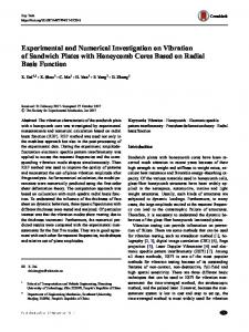
This result indicates that, at best, the maximum power extractable is bounded at 16/27 or 59.3% of the upstream available power. The Betz limit is based on arguments of linear momentum theory; however, Betz’s analysis does not account for angular momentum. Hermann Glauert used the angular momentum relationship and derived a new limit [7, 8, 9]. He found that the maximum extractable power was severely impacted by tip speed ratio as it approached zero, and that the maximum extractable power approached the Betz limit as tip speed ratio approached infinity. The derivation [10] is lengthier than the Betz limit derivation, but both derivation results are summarized in Figure 3.
7
Turbine Performance Parameters and Dimensionless Coefficients Hydrokinetic turbines are designed for a mean upstream flow velocity 𝑉𝑢𝑝 and a rotor rotation rate 𝜔. One important output parameter is the shaft power produced by the rotor, 𝑃𝑠 . This will always be less than the available hydraulic power, thus 𝑃𝐻 > 𝑃𝑠 . These two relations are shown in equation (8) 𝑃𝐻 =
𝑃𝑠 = 𝜏𝜔
𝜋 2 3 𝜌𝐷 𝑉 8 𝑡 𝑢𝑝
(8)
where 𝜏 is the torque produced by the rotor, 𝜌 is the fluid density, 𝐷𝑡 is the rotor’s diameter, and 𝑉𝑢𝑝 is the mean upstream open flow velocity. The power coefficient (𝐶𝑃 ) relates the amount of shaft power produced to the available hydraulic power. As previously mentioned, this power coefficient is bounded by limits derived by Betz and Glauert. The thrust coefficient (𝐶𝑇 ) is a dimensionless representation of the axial force on the rotor blades. This should not be confused with the drag coefficient (𝐶𝐷 ), which is the force parallel to the blade’s relative incoming flow. Lift 0.7
Power Coefficient: Cp [-]
0.6 0.5 0.4 0.3 0.2 Betz Limit
0.1
Glauert Limit
0 0
1
2
3
4
5
6
7
8
Tip Speed Ratio: λ [-]
Figure 3. Betz and Glauert Limits as a Function of Tip Speed Ratio 8
9
10
coefficient (𝐶𝐿 ) is perpendicular to the relative incoming flow. These definitions are depicted in equation (9) 𝐶𝑃 =
2𝑇 𝐶𝑇 = 𝜋 2 2 4 𝜌𝐷𝑡 𝑉𝑢𝑝
𝑃𝑆 𝑃𝐻
2𝐿 𝐶𝐿 = 𝜋 2 2 4 𝜌𝐷𝑡 𝑊
2𝐷 𝐶𝐷 = 𝜋 2 2 4 𝜌𝐷𝑡 𝑊
⃑⃑⃑ = 𝑉 ⃑ − 𝑟𝜔 𝑊 ⃑
(9)
⃑⃑⃑ is the where 𝑇 is the thrust force, 𝐿 is the lift force, 𝑊 is the relative oncoming velocity, 𝑊 ⃑ is the absolute oncoming velocity, 𝑟 is the radial relative oncoming velocity vector, 𝑉 position on the rotor, and 𝜔 ⃑ is the rotor’s rotation rate vector. The performance characteristics are a function of tip speed ratio (𝜆), the ratio of rotational tip velocity of a rotor to the oncoming flow velocity. Another important design characteristic is solidity (𝜎), defined as the ratio of chord length (𝑐) to the space between blades (𝑠). 𝜆=
𝑟𝜔 𝑉𝑢𝑝
𝜎=
𝑐 𝑠
𝑠=
2𝜋𝑟 𝑍𝐵
(10)
Here, 𝑍𝐵 is the number of rotor blades. Conventional hydropower characterizes turbines by head (𝐻), a measure of pressure in lengths of fluid, required to operate the unit. To allow for comparison, the head required by the hydrokinetic turbine can be estimated based on the dynamic pressure absorbed by the rotor. If one sets the both relations in equation (8) equal and solve for the velocity lost (𝑉𝑙 ) through the rotor, the head used by the hydrokinetic turbine (𝐻𝑟𝑜𝑡 ) can be calculated as shown equation (11) 2
8𝜏𝜔 𝑉𝑙 = √ 𝜋𝜌𝐷𝑡2 3
𝐻𝑟𝑜𝑡
9
1 8𝜏𝜔 3 = ( ) 2𝑔 𝜋𝜌𝐷𝑡2
(11)
where 𝑔 is the local gravitational constant. This calculation of head allows the use of standard quantities that compare various types of turbomachinery. These quantities are specific speed (𝑁𝑆 ), unit flow or discharge (𝑄11), unit speed (𝑁11 ), and unit power (𝑃11 ). 𝜋 𝑄 = 𝐷𝑡2 𝑉𝑙 4
1
𝑁𝑆 =
ω𝑄 2 3
(𝑔𝐻𝑟𝑜𝑡 )4
𝑄11 =
𝑄 √𝐻𝑟𝑜𝑡 𝐷𝑡2
𝑁11 =
𝑁𝐷𝑡 √𝐻𝑟𝑜𝑡
𝑃11 = 𝐶𝑃 𝑄11
(12)
Here, 𝑄 is the volume flow rate through the rotor and 𝑁 is the rotation rate in RPM. Note that these quantities are dimensional; however, the dimensions are unimportant and by practice are dropped.
Meridional Geometry
Figure 4. Example of A. Meridional View and B. Full View for a Pump-turbine Blade It is most convenient in rotating machinery to describe aspects of the system in a cylindrical coordinate system. During blade design, an 𝑟, 𝑧 projection of the blade called the meridional geometry is typically employed. Figure 4 depicts a comparison of the meridional view and full view of a pump-turbine. The same can be used to create a hydrokinetic turbine blade. Inverse-design Methodology Some design parameters must be assumed a priori to the design process. These input 10
variables are shown in Table 1. First, the tip diameter (𝐷𝑡 ), hub diameter (𝐷ℎ ), and mean diameter (𝐷𝑚 ) are calculated. A rough estimate of the required tip diameter (𝐷𝑡∗ ) is calculated as shown in equation (13). This relationship is derived from the fluid’s power flux through the rotor blade. This equation assumes that there is no hub, therefore the result must be rounded up to account for the area lost by the hub. Once the rounded tip diameter (𝐷𝑡 ) is selected, the hub diameter is predicted. The selected hub and tip diameters are used to calculate the mean diameter. The mean diameter is where the blade angles will be prescribed for the preliminary design. Multiple diameters between the hub and tip can be used if more control of the blade angles is desired.
Table 1. Input design variables selected a priori Input Variable 𝑃 𝐶𝑃 𝑈 𝜔 𝑍𝐵 𝜎 𝑡
𝐷𝑡∗ ≅ √
8𝑃 𝐶𝑃 𝜋𝜌𝑈 3
Description designed mechanical power output [ W ] designed power coefficient [ - ] designed free stream velocity [ m s-1 ] designed rotation rate [ rad s-1 ] designed number of blades [ - ] designed solidity [ - ] designed blade thickness [ m ]
𝐷ℎ ≅ √𝐷𝑡2 −
8𝑃 𝐶𝑃 𝜋𝜌𝑈 3
1 𝐷𝑚 = √ (𝐷𝑡2 − 𝐷ℎ2 ) 2
(13)
Once the mean diameter has been selected, the relative flow angles to the rotating frame of reference of the turbine can then be determined. A simplifying assumption used is that the relative flow angles entering and leaving the turbine are only functions of radial distance. This means that the relative flow angle incident to the leading edge is the same as 11
the deviation of the flow from the trailing edge (𝛽1 = 𝛽2 = 𝛽). This leaves the local tip-speed ratio (𝜉) and relative flow angle to be calculated from equation (14) 𝜉=
1 𝐷 𝜔 2 𝑚
𝑈
𝛽 = tan−1 𝜉
𝛽 ′ = 𝛽 + 24.874𝜉 −0.876
(14)
The relative blade angles can then be evaluated. Since the relative incidence and deviation flow angles are equal, the leading edge and trailing edge relative blade angles are equal as well (𝛽1′ = 𝛽2′ = 𝛽′), thus the relative blade angle is equal to the stagger angle (𝛽 ′ = 𝜓). Cebrián et al. [11] empirically related the relative blade angle to the relative flow angle and the local tip-speed ratio for maximum pressure loading in flat plate cascades as seen in equation (14). Finally, the mean chord length, axial blade length, and wrap angle are determined. The circumferential spacing between blades (𝑠) is calculated as shown in equation (15). The solidity chosen a priori is used to calculate the mean chord length. The axial blade length and wrap angle are determined once the mean chord length is calculated. 𝑠=
𝜋𝐷𝑚 𝑍𝐵
𝑐 = 𝜎𝑠
Δ𝑚 = 𝑐 cos 𝜓
Δ𝜃 =
2𝑐 sin 𝜓 𝐷𝑚
(15)
Literature Review Hydrokinetic turbines are a popular research topic, with engineers investigating multiple configurations. Batten et al. [12, 13, 14] used a blade element methodology (BEM) approach for horizontal axis tidal turbines. They validated their method using a scaled model in a cavitation tunnel, and concluded that their BEM model agreed with their experiments. Mukherji et al. [15] compared BEM with CFD for a horizontal axis hydrokinetic turbine, and determined the effect of solidity, angle of attack, and number of blades on power generation. Myer and Bahaj [16] conducted experiments on a horizontal axis turbine and concluded that 12
the blade twist distribution, centrifugal force at the surface of the blade, lift and drag performance, and rotor yaw angle affect the stall delay of the hydrofoil sections and thus can affect the power output from the rotor. Hwang et al. [17] studied a vertical axis turbine that actively controlled blade attack to maximize power output and improve self-start. They showed that by individually controlling each blade’s attack based on the oncoming flow that there was a 25% improvement in performance compared to pure cycloidal motion for the same operating conditions. The same design principles used for wind turbines, marine propellers, and propeller turbines can be used in hydrokinetic designs. Massouh and Dobrev [18] studied the vortex wake behind a horizontal axis wind turbine in a wind tunnel and compared the results to CFD analysis. Their results showed that the tip vortices are not limited to a cylindrical surface as what is predicted from linear propeller theory and expand radially as they move downstream, thus increasing the diameter of the streamtube that the turbine is located within. Vermeer et al. [19] also studied the wake characteristics behind wind turbines in the near and far wake regions. Alexander et al. [20] have studied axial-flow, flat blade propeller turbines that can be manufactured in underdeveloped countries to provide sustainable power generation for communities. They have shown that simplifying the blade geometry of propeller turbines can still produce significant power and can be easier to manufacture for locations where advanced machining may not be possible. The work of Alexander et al. [20] was validated and compared with an Archimedean screw turbine by Schleicher et al. [21], who have studied different micro-hydro systems [22, 23]. Singh and Nestmann [24] experimentally studied the part-load performance of small axial-flow propeller turbines and found that modifying the exit tip region of their studied propellers consistently showed an increase in flow and output 13
shaft power and thus the hydraulic efficiency of the blades. Hayati et al. [25] investigated the effect of rake angle on marine propeller performance and concluded that increasing the rake angle improved the thrust performance of conventional propellers. Even though these propellers are imposing energy onto the fluid and not absorbing the energy, it is possible that adjusting the rake angle may improve thrust performance in the energy absorbing case. Objectives and Outline of Dissertation Work This dissertation is structured into seven chapters. Chapter 1 provides an introduction to the field of hydropower and hydrokinetics. This chapter starts by motivating the studies conducted in this manuscript. Hydrokinetic turbines and factors pertaining to them such as their types, performance metrics, and design methods are then discussed. A literature review on the state of hydrokinetics and hydropower systems is presented. In Chapter 2, the Reynolds Averaged Navier-Stokes equations are developed for the absolute reference frame as well as a rotating reference frame. The k-ω Shear Stress Transport turbulence model is then discussed. The concept of the finite volume method is introduced, and the computational domain studied in this manuscript is presented along with boundary conditions. Chapter 3 introduces the optimization methodology studied in this dissertation. First, optimization concepts are introduced. Different types of optimization methods and their shortcomings are discussed. The optimization method used in Chapter 4 through Chapter 7 is then introduced. A verification test problem proves that the optimization method is able to find global optimum conditions given a set of three complex output responses. In Chapter 4, the optimization methodology is tuned and characterized. Simulations are conducted for a 2.25 m/s free-stream flow in a nearly infinite medium. The adaptive 14
response surface optimization methodology explores hub diameter, tip diameter, axial blade length, and wrap angle to optimize a propeller-type hydrokinetic turbine for a power generation goal of 500 Watts while exerting less than or equal to 125 lbf of thrust on the blades. Two starting points for the optimization are selected: one near the expected optimum condition and one far from this expected condition. The design space for the adaptive response surface methodology is deviated 5%, 10%, and 15% from the starting conditions. This yields six different optimizations, all of which are trying to obtain the same optimum conditions in the least amount of adaptions to the response surface. Chapter 5 takes what was learned in Chapter 4 to optimize propeller-type hydrokinetic turbines for different operating conditions and design goals. This includes designs for shallow versus deep waters, slow versus fast flow speeds, and small versus large power generation goals. The shallow water designs focus on water channels 10 feet (3 m) in hydraulic diameter with the rotation axis submerged 2.5 feet while the deep water designs will focus on channels 40 feet (12 m) in hydraulic diameter submerged 10 feet. Slow fluid speeds are investigated at 1.5 m/s and fast speeds at 3 m/s. Small power generation goal designs of 0.25 kW and a large generation goals of 2 kW are investigated. The optimized designs are compared and trends among design characteristics will be determined between the different operating and generation conditions. Chapter 6 investigates the use of blade profile curvature. The propeller designs in the previous chapters had zero curvature in the designed profiles. Bezier splines are used to parameterize wrap angle as a function of meanline to add curvature to a blade design. The curvature is controlled at the hub and tip diameters. The optimized design is compared to the starting design for its performance improvement. 15
Chapter 7 uses the optimization method to hydraulically optimize a small pumpturbine design. The performance of the starting and optimize designs are compared as well as their flow fields through the mid-plane of the runner. This chapter illustrates that the optimization method works for different hydraulic turbomachine types. Chapter 8 concludes this manuscript and summarizes the conclusions from the previous chapters.
16
Chapter 2
REYNOLDS AVERAGED NAVIER-STOKES FLOW MODEL
The flow field through and around hydrokinetic turbines directly influences performance parameters such as power and thrust. An appropriate flow field model is necessary to accurately capture these performance characteristics, let alone attempt an optimization of these performance characteristics. In Chapter 1, a 1D inverse design methodology was proposed for propeller-type hydrokinetic turbines. This chapter focuses on deriving the 3D governing equations to analyze these propeller-type designs. Flow Model The Reynolds Averaged Navier-Stokes equation is derived in this section for an absolute frame of reference. This derivation is then extended to a rotating frame of reference with respect to the blade’s rotation speed, thus providing a steady flow model for flow near the rotor. These equations are formulated under the assumption that the flow field is incompressible, allowing fluid density to be considered constant throughout the flow field. Reynolds decomposition is employed, allowing the velocity components in the NavierStokes equation to be broken into time-averaged and fluctuating components as shown in equation (16). The Navier-Stokes equation is Reynolds-averaged, or time-averaged, for statistically stationary turbulence as defined in equation (16). 𝑢(𝑥𝑖 , 𝑡) = 𝑢̅(𝑥𝑖 ) + 𝑢′ (𝑥𝑖 , 𝑡)
1 𝑡+𝑇 ∫ 𝑢(𝑥𝑖 , 𝑡1 )𝑑𝑡1 𝑇→∞ 𝑇 𝑡
𝑢̅𝑖 (𝑥𝑖 , 𝑡) = lim
(16)
Absolute Frame of Reference The flow model starts from conservation of mass and the Navier-Stokes equation 17
(conservation of momentum) for incompressible flow in a continuous medium. Note that body forces have been neglected from the Navier-Stokes equation. 𝜕𝑢𝑖 =0 𝜕𝑥𝑖
𝜕𝑢𝑖 𝜕𝑢𝑖 1 𝜕𝑝 𝜕 2 𝑢𝑖 + 𝑢𝑗 =− +𝜈 𝜕𝑡 𝜕𝑥𝑗 𝜌 𝜕𝑥𝑖 𝜕𝑥𝑗 𝜕𝑥𝑗
(17)
Reynolds decomposition is applied to these equations by substituting the definition from equation (16) into equation (17). This results in equation (18). 𝜕𝑢̅𝑖 𝜕𝑢′𝑖 + =0 𝜕𝑥𝑖 𝜕𝑥𝑖 𝜕(𝑢̅𝑖 + 𝑢𝑖′ ) 𝜕𝑢̅𝑖 𝜕𝑢′𝑖 𝜕𝑢̅𝑖 𝜕𝑢′𝑖 + 𝑢̅𝑗 + 𝑢̅𝑗 + 𝑢′𝑗 + 𝑢′𝑗 𝜕𝑡 𝜕𝑥𝑗 𝜕𝑥𝑗 𝜕𝑥𝑗 𝜕𝑥𝑗
(18)
1 𝜕(𝑝̅ + 𝑝′) 𝜕 2 (𝑢̅𝑖 + 𝑢𝑖′ ) =− +𝜈 𝜌 𝜕𝑥𝑖 𝜕𝑥𝑗 𝜕𝑥𝑗 Once the equations are Reynolds decomposed, these equations are time averaged. It is ̅ 𝑖 = 0 and 𝑢̿𝑖 = 𝑢̅𝑖 . important to note that 𝑢′ 𝜕𝑢̅𝑖 =0 𝜕𝑥𝑖 ̅̅̅̅̅̅̅ 𝜕𝑢̅𝑖 𝜕(𝑢̅𝑗 𝑢̅𝑖 ) 𝜕(𝑢′ 1 𝜕𝑝̅ 𝜕 2 𝑢̅𝑖 𝑗 𝑢′𝑖 ) + + =− +𝜈 𝜕𝑡 𝜕𝑥𝑗 𝜕𝑥𝑗 𝜌 𝜕𝑥𝑖 𝜕𝑥𝑗 𝜕𝑥𝑗
(19)
The resulting equation looks strikingly similar to the Navier-Stokes equations at the beginning of the derivation; however, a new term has appeared involving ̅̅̅̅̅̅ 𝑢𝑗′ 𝑢𝑖′ . There is no prescription for this time-averaged fluctuation transfer, thus the average flow quantities cannot be calculated. This is what has fundamentally driven turbulence modeling for the past few decades: prescribing a relationship for ̅̅̅̅̅̅ 𝑢𝑗′ 𝑢𝑖′ .
18
Rotating Frame of Reference Solving these equations in the absolute frame of reference is difficult in turbomachinery. The flow field around the rotor is highly unsteady in this inertial reference frame. It is easier to solve these equations in a relative reference frame to the rotor’s rotational speed, transforming the unsteady inertial frame into a steady non-inertial frame. This is accomplished by including terms in the transport equations for centrifugal and Coriolis forces. Conservation of mass and momentum takes the form of equation (20). 𝜕𝑤𝑖 =0 𝜕𝑥𝑖 𝜕𝑤𝑖 𝜕𝑤𝑖 1 𝜕𝑝 𝜕 2 𝑤𝑖 + 𝑤𝑗 =− − 2𝜖𝑖𝑘𝑙 Ω𝑘 𝑤𝑙 − 𝜖𝑖𝑘𝑙 𝜖𝑙𝑠𝑡 Ω𝑘 Ω𝑠 𝑥𝑡 + 𝜈 𝜕𝑡 𝜕𝑥𝑗 𝜌 𝜕𝑥𝑖 𝜕𝑥𝑗 𝜕𝑥𝑗
(20)
Here, 𝑤 is the relative velocity field to the rotating reference frame, 𝜖 is the permutation symbol, and Ω is the angular speed of the reference frame. A similar process as the absolute reference frame Reynolds-averaged Navier-Stokes derivation, leading to the resulting governing equations shown below. 𝜕𝑤 ̅𝑖 =0 𝜕𝑥𝑖 ̅̅̅̅̅̅̅̅ ̅𝑗 𝑤 ̅ 𝑖 ) 𝜕(𝑤′ 𝜕𝑤 ̅ 𝑖 𝜕(𝑤 𝑗 𝑤′𝑖 ) + + 𝜕𝑡 𝜕𝑥𝑗 𝜕𝑥𝑗
(21)
1 𝜕𝑝̅ 𝜕 2𝑤 ̅𝑖 =− − 2𝜖𝑖𝑘𝑙 Ω𝑘 𝑤 ̅ 𝑙 − 𝜖𝑖𝑘𝑙 𝜖𝑙𝑠𝑡 Ω𝑘 Ω𝑠 𝑥𝑡 + 𝜈 𝜌 𝜕𝑥𝑖 𝜕𝑥𝑗 𝜕𝑥𝑗 This formulation also has the time-averaged fluctuation transfer term ̅̅̅̅̅̅̅̅ 𝑤′𝑗 𝑤′𝑖 similar to the formulation in the absolute reference frame.
19
Turbulence Modeling The time averaged fluctuation transfer term that appears in the Reynolds-averaged ′ ′ ̅̅̅̅̅̅ Navier-Stokes equation, −𝑢 𝑗 𝑢𝑖 , is commonly referred to as the specific Reynolds stress
tensor denoted by 𝜏𝑖𝑗 . This is a symmetric tensor containing six unknown quantities leaving the flow governing equations as an open system of equations. Turbulence modeling aims to derive relations for these six components of the specific Reynolds stress tensor, thus closing the system of equations. One common approach to turbulence modeling is using the Boussinesq eddyviscosity approximation to compute the specific Reynolds stress tensor and the mean strainrate tensor. Here, it is assumed that there is a linear relationship between stress and strain in the flow field. This is accomplished by introducing the turbulent kinetic energy and kinematic eddy viscosity quantities, allowing the specific Reynolds stresses to be defined as in equation (22). 𝑘=
1 ′ ′ ̅̅̅̅̅̅ 𝑢𝑢 2 𝑖 𝑖
2 𝜕𝑢𝑖 𝜕𝑢𝑗 ′ ′ ̅̅̅̅̅̅ 𝜏𝑖𝑗 = −𝑢 + ) 𝑗 𝑢𝑖 = 𝑘𝛿𝑖𝑗 − 𝜈𝑡 ( 3 𝜕𝑥𝑗 𝜕𝑥𝑖
(22)
Here, 𝑘 represents turbulent kinetic energy, 𝛿𝑖𝑗 is the Kronecker delta, and 𝜈𝑡 is the kinematic eddy-viscosity. Kinematic eddy-viscosity is defined differently depending on the turbulence model employed. One such turbulence model that is based on the Boussinesq eddy-viscosity approximation is Menter’s k-ω Shear Stress Transport (SST) [26, 27] two-equation eddyviscosity model. This model offers improved prediction of adverse pressure gradients in the near wall region as compared to the standard k-ω and k-ε models by incorporating Bradshaw’s observation that turbulent shear stress is proportional to the turbulent kinetic 20
energy in the wake region of the boundary layer [27]. The equations for kinematic eddy viscosity, turbulent kinetic energy, and specific dissipation rate are shown in equation (23). 𝜈𝑇 =
𝛼1 𝑘 max(𝛼1 𝜔, 𝑆𝐹2 )
𝜕𝑘 𝜕𝑘 𝜕𝑈𝑖 𝜕 𝜕𝑘 + 𝑈𝑗 = 𝜏𝑖𝑗 − 𝛽 ∗ 𝑘𝜔 + [(𝜈 + 𝜎𝑘 𝜈𝑇 ) ] 𝜕𝑡 𝜕𝑥𝑗 𝜕𝑥𝑗 𝜕𝑥𝑗 𝜕𝑥𝑗 𝜕𝜔 𝜕𝜔 𝜕 𝜕𝜔 + 𝑈𝑗 = 𝛼𝑆 2 − 𝛽𝜔2 + [(𝜈 + 𝜎𝜔 𝜈𝑇 ) ] 𝜕𝑡 𝜕𝑥𝑗 𝜕𝑥𝑗 𝜕𝑥𝑗 1 𝜕𝑘 𝜕𝜔 + 2(1 − 𝐹1 )𝜎𝜔2 𝜔 𝜕𝑥𝑖 𝜕𝑥𝑖
(23)
Here, 𝜈𝑇 is the turbulent viscosity, 𝜈 is the kinematic viscosity, 𝑘 is the turbulent kinetic energy, 𝜔 is the specific dissipation rate, 𝛼1 is a closure coefficient, 𝑈 is the velocity, and 𝑆 is the mean rate-of-strain tensor. For the sake of brevity, the blending functions 𝐹1 and 𝐹2 are not shown but the implemented model uses the original implementation of the k-ω SST turbulence model. Numerical Method Finite Volume CFD Introduction There are many computational approaches to solve the governing equations in fluid dynamics. All methods convert the governing partial differential equations and boundary conditions into a system of discrete algebraic equations commonly referred to as the discretization stage. Examples of discretization methods include finite difference, finite element, finite volume, and spectral methods. Once discretized, numerical methods are implemented to obtain a solution to the system of algebraic equations. Two popular methods for discretizing these governing equations are the finite volume and finite difference methods. The finite difference method discretizes the governing 21
equations in the weak form of the partial differential equations. This method is easy to code and is usually the first glimpse students get at the world of computational fluid dynamics. The finite difference method of discretization is difficult when complex geometries are investigated. The finite volume method has a significant advantage over the finite difference method when complex geometries are investigated since it uses control volumes instead of grid intersection points. The finite volume method solves the governing equations in the strong form, and is a conservative method as long as the surface integrals applied at boundaries are the same as the control volumes sharing that boundary. A disadvantage of the finite volume method is that higher order differencing schemes than second order are difficult in three dimensions. Most modern commercial solver packages use the finite volume method to solve governing equations in CFD. The backbone of the finite volume method is control volume integration with Gauss’ divergence theorem. This allows the first-order partial derivative of a generic flow variable 𝜙 in the x-direction as depicted in equation (24). 𝑁
𝜕𝜙 1 𝜕𝜙 1 1 = ∭ 𝑑∀= ∬ 𝜙𝑑𝐴𝑥 ≈ ∑ 𝜙𝑖 𝐴𝑖𝑥 𝜕𝑥 Δ∀ 𝜕𝑥 Δ∀ Δ∀
(24)
𝑖=1
Here, ∀ is the discretized volume, 𝐴𝑖𝑥 is the x-direction projection of the discretized volume’s 𝑖th face, and 𝑁 is the number of faces on the discretized volume. Implemented Methods The computations performed in this dissertation used the steady RANS equations with the k-ω SST turbulence model. Pressure-velocity coupling was accomplished using the SIMPLE method. Gradient schemes were calculated with using second order Gaussian integration with a second order linear interpolation scheme (central differencing). Surface 22
normal gradients were calculated with an explicit non-orthogonal correction scheme. Lapacians were calculated using Gaussian integration, with the linear interpolation and corrected surface normal gradient schemes, providing a conservative, unbounded second order approximation. The divergence between face flux and momentum used Gaussian integration with a bounded, second order linear-upwind scheme. The divergence between face flux and turbulence parameters used Gaussian integration with a bounded, second order limited-linear TVD scheme using the Sweby limiter. All flow variables were solved with a linear, iterative, geometric-algebraic multi-grid (GAMG) method. A Gauss-Seidel smoother was used for all solved flow variables with three post sweep (as the mesh is refined in the GAMG solver) and thirty sweeps at the finest mesh level. In addition, the pressure correction solver used one pre sweep as the mesh is coarsened by the GAMG solver. The flow variables were also under-relaxed by 0.7 for all flow variables except for pressure which was under-relaxed by 0.3. Boundary conditions Figure 5 labels the computational domains and boundary conditions for the RANS equations. The entire computational domain is comprised of two subdomains: the outer subdomain termed the river domain and an inner cylindrical subdomain coined the turbine domain. The turbine domain is located inside the river domain as depicted in Figure 5. Each of these subdomains are solved in different reference frames. The river domain is solved in the inertial absolute reference frame while the turbine domain is solved in the non-inertial relative reference frame with respect to the turbine’s rotational speed. For unstructured tetrahedral mesh simulations, the connection between these two domains is conformal; however for structured hexahedral meshes this domain interface is 23
24
Figure 5. Boundary Conditions for the RANS Simulations
non-conformal and a grid interpolation methodology is employed between these two domains. This method, called the Generalized Grid Interface (GGI), couples two nonconformal mesh interfaces into a single domain at the matrix level of the solver by using a set of weight factors to balance the fluxes at the GGI interface [28]. More details about the GGI method are given in the Numerical Method section. The river domain is modeled as a cylindania (half-cylinder). The curved portion of the domain is coined as the river bed and modeled as a no-slip, hydraulically smooth wall. The flat rectangular surface of the cylindania is termed the free surface; however, the surface is not deformable as the free surface in channel flow would be. It is modeled as a fixed, slip wall to mimic the zero shear effect normally present at the free surface of channel flows. The semi-circular face upstream of the turbine is the inlet for the computational domain. The mean velocity (𝑉), turbulent intensity (𝐼), a dissipation length scale (𝑙), and a zero gradient condition for pressure are prescribed here as defined in equation (25). 𝜌𝑉𝐷𝐻 −1⁄8 𝐼 = 0.16 ( ) 𝜇
4𝐴 𝑙 = 0.07𝐷𝐻 = 0.07 ( ) 𝑃𝑤𝑒𝑡
(25)
Here, 𝐷𝐻 is the hydraulic diameter of the inlet, 𝐴 is the area of the inlet, 𝑃𝑤𝑒𝑡 is the wetted perimeter of the inlet, and 𝜇 is the dynamic viscosity. The semi-circular face downstream of the turbine is the outlet. A gauge pressure and zero gradient conditions for velocity and turbulence parameters are set here. In the turbine domain, the blades, hub, leading and trailing cones are no-slip, hydraulically smooth walls. The blades and the hub boundaries are no-slip conditions relative to the rotating reference frame while the leading and trailing cones are no-slip wall in the absolute reference frame or counter rotating walls to the rotating reference frame. 25
Chapter 3
OPTIMIZATION METHODOLOGY
Introduction to Optimization Optimization strategies are vital to the design process. The simplest approach to optimization is to change one of the design variables at a time while holding other design variables constant. This method is highly inefficient and rarely arrives near an optimized design [29]. It is better to approach optimization from a more systematic perspective. This usually entails determining any objective functions, or goals, for the optimization, whether the aim is to minimize or maximize the objective function, any constraints the objective functions must obey, and the bounds on the investigated design space. The objective functions can be linear or non-linear, implicit or explicit functions. Design variables can be continuous or discrete. The choice of optimization technique will ultimately depend on these factors. Optimization algorithms can be divided into two basic groups: local or global [30]. Local optimization methods use gradients to search for local optimum conditions. These methods generally operate in two steps. In the first step, the algorithm determines the output of the objective function around the starting design point. It then estimates the gradients and determines the best direction to move the design variables. In the second step, the design variables are changed to move in the direction determined in step one until no further progress can be made. Examples of local optimization include Newton’s method, variable metric methods, Sequential Unconstrained Minimization Techniques (SUMT), and direct or constrained methods [30]. These methods excel when there are more than
26
approximately 50 design variables; however, they are only capable of finding local extrema and are dependent on the initial design variables. Many optimization problems have multiple extrema, making it difficult to arrive at the true global minima or maxima using local optimization techniques. One way to circumvent this problem is to use multiple starting points for the local optimization method; however, using a global optimization method may be better suited for this task. Global optimization methods have a better chance of finding the true global optimum. Global optimization algorithms are typically used when the number of design variables is less than 50. Computationally speaking, global optimization algorithms are more expensive compared to local optimization algorithms because the number of objective function evaluations increases rapidly with the number of design variables. A response surface optimization methodology is a form of a function approximation optimization that uses an experimental design combined with a regression model to approximate the behavior of a system. This optimization method was first pioneered in the 1950s by Box and Wilson [31]. The optimization methodology has gained popularity in recent years and has been applied to turbomachinery design problems. Jang et al. [32] applied this method to optimization of a single stage axial compressor and Kim et al. [33] used this methodology on a centrifugal compressor. Li et al. [34], Rubechini et al. [35], and Cravero and Macelloni [36] optimized multistage turbines with a response surface methodology. The Optimization Algorithm The employed optimization flow chart is depicted in Figure 6. The first step in the design optimization scheme is to define the goals of the optimization. These design goals could be to increase torque, increase the designed tip-speed ratio, reduce thrust, and minimize 27
Figure 6. Adaptive Response Surface Optimization Flow Chart tip diameter. Once the goals of the optimization are set, the geometric parameters for the system must be selected. The next step is to define the limits on the design space to be studied. This can be difficult to do on the first design iteration because the global minima or maxima may not actually be in that range. Therefore, for the first design iteration it is suggested that the design space be as large as possible. If at the end of the first design iteration the design goals are met on the edge of the design space for any variable, the design space should be adjusted further in that direction in an attempt to bring the maxima or minima into the design space. An appropriate experimental design is then selected such as a central composite design, optimal space-filling design, or any of their variants. In this dissertation, a central 28
composite design was used. The simulations are then solved and post-processed for performance characteristics relevant to the optimization goals. These results are regressed using a non-parametric regression, which is a meta-modeling technique capable of representing highly non-linear outputs relative to inputs. Each regression is then screened through and an optimal result is estimated. Here, the optimized result can be further tested if the solution is structurally sound. This process is further repeated until the parameterized geometric model has converged on an optimal solution within a given tolerance between successive design iterations. Verification Test Problem This optimization methodology was tested for robustness on three functions: a parabolic function, Rastrigin’s function, and a function with a large, flat valley in the vicinity of its global minimum. These functions are depicted in equation (26)Figure . 𝑓1 (𝑥1 , 𝑥2 ) = 𝑥12 + 𝑥22 𝑓2 (𝑥1 , 𝑥2 ) = 20 + 𝑥12 + 𝑥22 − 10[cos(2𝜋𝑥1 ) + cos(2𝜋𝑥2 )] 2
𝑓3 (𝑥1 , 𝑥2 ) = 100((𝑥2 + 1) − (𝑥1 + 1)2 ) + (1 − (𝑥1 + 1))
(26) 2
All three functions have global minimums at 𝑓𝑖 (0,0) = 0. The optimization algorithm was used to find the global minimum for all three equations at the same time. The Rastrigin function provides an interesting challenge for many optimization algorithms as it has many local minimums within the design space. This can prove especially challenging for gradient based methods. The valley function also adds difficulty to the optimization problem because of the large region where the derivative is nearly zero. The first step from Figure 6 is to start from a preliminary design solution. In this case, the starting point for this verification study was (𝑥1 , 𝑥2 ) = (7, −7). Relatively speaking, this 29
was far away from the global minimum. This was chosen to test the merit of the optimization method even if a poor initial guess at the solution is made. The next step is to define the optimization goals. The goal of this optimization is to find the global minimum solution for all three functions, while evaluating the output to all three functions simultaneously. This further adds complexity to the optimization to try and find the global optimum conditions. Both 𝑥1 and 𝑥2 were selected as the influential parameters to be studied. The design space investigated for these equations ranged from -10 to 10 for both 𝑥1 and 𝑥2 . A central composite design consisting of nine experiments was used, with a starting deviation of 1.4 between experiments was used. This deviation was refined once it had relatively converged on the global minimum. This refinement was done six times to a final deviation of 7 × 10⁻⁶ . More discussion about deviation and its definition can be found in Chapter 4. Solving the experiments done by evaluating each function for the experimental design points. This is not easy when the evaluation is a computer simulation that requires hours to days to compute the output. Since the output is a function in this verification problem, the output is known after a simple function evaluation. A non-parametric regression is applied to the experiments, and if other experimental batches were previously performed they are included in the regression as well. New optimum conditions are then found by screening the regression. If this were a turbine optimization problem, it may now be useful to check the newly predicted optimum design with a structural FEA solver to ensure a valid physical solution. This process is repeated until the predicted optimum result has converged on an optimum solution with successive optimization iteration. The optimization methodology was capable of finding the global minimum within an
30
Figure 7. A. Parabolic Function B. Rastrigin's Function C. Valley Function
Figure 8. Convergence of A. 𝑥1 , B. 𝑥2 , C. Normalized 𝑥1 , and D. Normalized 𝑥2 as a Function of Experiment Number 31
accuracy of ±1 × 10⁻⁵ . Fifty-seven batches of experiments were conducted, with each batch consisting of nine experiments for a total of 513 experiments. A more precise prediction of the global minimum can be obtained with more experimental batches; however, the result is clear than the optimization methodology was capable of honing in on the global minimum even given the complexity of the output functions.
32
Chapter 4
APPLICATION OF THE OPTIMIZATION METHODOLOGY TO HYDROKINETIC TURBINES
Motivation The optimization methodology presented in the previous chapter will be used to determine more hydraulically optimum propeller-type hydrokinetic turbines. The goal of this chapter is to explore the adaptive response surface methodology and learn how to tune it to find optimum designs efficiently. An efficient optimization strategy will find the global optimum result while minimizing the number of simulations needed to find this optimum. The simulations needed to populate the response surface are determined by a central composite design of experiments. This experimental design guarantees a second order accurate regression of the output results. This chapter aims to identify how far apart should these design points be in order to both arrive at the optimum result as fast as possible, but still have an acceptable accuracy in identifying the optimum result. An example of a central composite design for to independent variables is depicted in Figure 9. If the deviation between experiments is high, a larger portion of the response surface is explored; however, it may also be too far apart and not capturing important trends in local phenomena between experiment design points. This can be rectified by simply choosing a smaller deviation between design points; however, a smaller portion of the response surface is explored and the number of experiments required arrive at the optimum will be substantially larger. If the design is already near the optimum design, it makes sense to have a small deviation in the experimental design. If it is unknown how close the design is to the optimum design, a larger deviation between experiments would seem appropriate. In this chapter, the 33
2
1.5
1
𝑥1 = 𝑥̅1 − 𝛿𝑥̅1
𝑥1 = 𝑥̅1 + 𝛿𝑥̅1
0.5
0 -2
-1.5
-1
-0.5
0
0.5
1
1.5
2
-0.5
-1
-1.5
-2
Figure 9. Example of a Central Composite Design for Two Independent Variables deviation between experiment design points will be explored for a design predicted to be nearly optimum and a design that is confidently far away from optimum conditions. The deviation for each experimental batch was parameterized as a mean value, plus or minus a percent of that mean value as depicted in Figure 9. Optimization Goals and Starting Designs The turbine rotor geometries in this study were optimized for a 2.25 m/s free stream velocity and a 150 RPM rotation rate. These designs were placed in a domain large enough that the blockage ratio was on the order of 1%. This was considered low enough to qualify as an infinite medium. The hub and tip diameters (𝐷ℎ and 𝐷𝑡 ), the axial blade height (Δ𝑚), and blade wrap angle (Δ𝜃) were investigated as the independent variables. The goal of the 34
optimization was to minimize the tip diameter and thrust on the turbine blades, while seeking a target power output of 500 Watts. A maximum of nine experimental batches will be performed. A nearly optimum and far from optimum design was used as the starting point for this investigation. In previous publications [22, 37], a preliminary design for a propeller-type hydrokinetic turbine was thoroughly numerically characterized. This design is expected to be nearly optimum and was used as the nearly optimum starting point for this study. Using the same design methodology, a far from optimum design was derived. This far optimum
Figure 10. A. and B. Far from Optimum and B. and C. Nearly Optimum Starting Designs 35
design was derived for 50 Watts at 1.5 m/s. The initial designs are pictured in Figure 10.
Table 2. Starting Design Parameters for the Optimization Study Near Optimum Design Far from Optimum Design 5.000 in 6.000 in 𝐷ℎ 21.000 in 13.750 in 𝐷𝑡 3.906 in 2.737 in Δ𝑚 94.86° 92.92° Δ𝜃
For both the nearly optimum and far from optimum designs, the deviation in the design space (𝛿) was investigated. Deviations of 5%, 10%, and 15% were investigated yielding six different optimizations for this study. The thought is that for the nearly optimum case, the 5% deviation in experimental design points will better predict the optimum result than the larger deviations. In the far from optimum case, the 15% deviation will yield a more optimum result and arrive there faster than the 5% deviation. Results and Discussions Refined CFD Spatial Convergence Spatial convergence was verified for the refined CFD domain using the Richardson extrapolation based Grid Convergence Index (GCI) method [38, 39, 40, 41]. This method provides an estimate of the error band on solution quantities due to discretization error. Simulations were conducted at the turbine’s design conditions on three successively refined meshes. These meshes contained 𝑁1 = 1,188,542 cells, 𝑁2 = 5,929,864 cells, and 𝑁3 = 14,607,868 cells. All simulation conditions were held constant for each mesh. A summary of this study is depicted in TABLE 3. The refinement ratio between meshes 𝑁2 and 𝑁1 as well as between meshes 𝑁3 and 𝑁2 are defined by 𝑟21 and 𝑟32 , respectfully. The solution quantities for torque and thrust are represented by 𝜙1 , 𝜙2 , and 𝜙3 for each respective mesh, 36
and 𝑝 is the observed order of convergence between the studied meshes. Based on the results of this convergence study and weighing computational costs, the 𝑁2 mesh was chosen to characterize the design. With the rate of convergence known, the extrapolated 21 value for the solution quantities (𝜙𝑒𝑥𝑡 ), the relative error (𝑒𝑎21 ), the extrapolated relative 21 21 error (𝑒𝑒𝑥𝑡 ), and the Grid Convergence Index for the 𝑁2 mesh (𝐺𝐶𝐼𝑓𝑖𝑛𝑒 ) were calculated.
The results show that there is a 2-3% error band on the calculated quantities of torque and thrust due to discretization.
TABLE 3. Sample calculations of discretization error 𝑁1 , 𝑁2 , 𝑁3 𝑟21 𝑟32 𝜙1 𝜙2 𝜙3 𝑝 21 𝜙𝑒𝑥𝑡 𝑒𝑎21 21 𝑒𝑒𝑥𝑡 21 𝐺𝐶𝐼𝑓𝑖𝑛𝑒
𝜙 = Torque [Nm] 1188542, 5929864, 14607868 1.709 1.351 34.5242 35.3426 35.2616 1.25 33.6621 2.4% 2.6% 3.1%
𝜙 = Thrust [N] 1188542, 5929864, 14607868 1.709 1.351 644.4971 636.9606 636.3088 1.02 654.8748 1.2% 1.6% 2.0%
Inlet and Outlet Verification and Wake Effect Results The location of the inlet and outlet boundary conditions was investigated to understand the numerical solution’s dependence on their placement. The outlet conditions were placed 10, 20, 30, and 40 turbine tip diameters downstream of the blade leading edges for a constant inlet length. The inlet boundary was placed 10 and 20 tip diameters upstream on the blade leading edges for a constant outlet length. 37
Norm. Axial Velocity at Rotation Centerline (Vz/Vup) [-]
10 Diameters
20 Diameters
30 Diameters
40 Diameters
1 0.875 0.75 0.625 0.5 0.375 0.25 0.125 0 -0.125 0
5
10 15 20 25 30 Normalized Outlet Length (Loutlet/Dt) [-]
35
40
Figure 11. Normalized Axial Velocity at the Rotation Axis versus Normalized Outlet Length Depicted in Figure 11 are plots of normalized axial velocity at the rotation axis versus normalized outlet length. The velocity was normalized to the inlet velocity and the outlet length was normalized to the tip diameter. The result indicates that for the studied outlet lengths, the location of the outlet boundary has no noticeable difference in the axial velocity field. Torque and thrust differed by at most 0.1% between these simulations compared to the 40 diameter outlet result. The wake from the rotor travels a significant distance downstream of the rotor. Its effect is so strong that even after 40 tip diameters the axial velocity at the rotation axis centerline has only redeveloped to 90.6% of the upstream inlet boundary velocity. It is not possible to discern if the axial velocity is asymptotically approaching the inlet velocity or a 38
10 Diameters
20 Diameters
Normalized Axial Velocity at Rotation Centerline (Vz/Vup) [-]
1.2 1 0.8 0.6 0.4 0.2 0 0
5 10 15 Normalized Inlet Length (Linlet/Dt) [-]
20
Figure 12. Normalized Axial Velocity at the Rotation Axis versus Normalized Inlet Length slightly smaller velocity due to energy extracted from the rotor. If the lost velocity is calculated from equation (11) and an area weighted average from the unaffected free-stream velocity and the lost velocity is performed, it is estimated the fully developed velocity will be 2.24 m/s. Plotted in Figure 12 is normalized axial velocity with respect to the inlet velocity versus normalized inlet length with respect to tip diameter. It is seen that the axial velocity along the rotation axis remains unaffected for inlets 10 and 20 tip diameters upstream of the blade leading edges. The inlet boundary would have to be located very far upstream in order for that constant, uniform flow velocity prescribed at this boundary to full develop. Then one would see a slight difference in the plotted axial velocity. 39
Optimization Results The optimization algorithm was iterated over nine simulations batches for both the near optimum start and far from optimum start. The input parametric design variables for this study are plotted as a function of experimental batch number in Figure 13 for the near optimum start and Figure 14 for the far from optimum start. Each experimental batch consisted of 27 simulations and were formulated based on a central composite design around the previous batch’s optimum result prediction. This yields a total of 243 rapid CFD simulations per investigated experimental design point deviation and starting points, for a grand total of 1,458 simulations for the entire study. The results depicted in Figure 13 and Figure 14 indicate that a converged solution in the sense that the input parametric variables did not change with subsequent experimental batch, was not strictly reached. One reason strict convergence was not reached was the lack of constraints applied to the input parametric design variables in the first few experimental design batches. The original goal of the optimization algorithm was to seek a design that produced exactly 500 Watts and to choose the design which accomplished this goal that produced the least amount of thrust. No constraint was placed on the tip diameter for these designs, nor was there a constraint on the efficiency of the design. This was an oversight that was corrected in the middle of the optimization algorithm. Constraints on the allowable limits of torque production and blade power coefficient (efficiency) were effective as of the fifth experimental batch. Goals to maximize the power coefficient and to minimize the rotor diameter were also in effect as of the fifth experimental batch. The effects of these added constraints and goals can clearly be seen in Figure 13B. The tip diameter after the fourth experimental batch drastically decreased in the near 40
optimum start simulations. The 10% and 15% deviations depict the tip diameter decreasing after the new goals and constraints were added to the optimization problem, and then jump back up near the starting tip diameter. This was probably a natural compensation by the optimization algorithm since it lacked simulation results for the smaller tip diameters, and the response surface predicted the optimization goals may possibly be met given the data that was available at that point in the optimization process. If given the opportunity to conduct more experimental batches, the input parametric variables would eventually converge on a
41
42
Figure 13. Convergence of A. Hub Diameter, B. Axial Blade Length, C. Tip Diameter, and D. Wrap Angle for the Near Optimum Design
43
Figure 14. Convergence of A. Hub Diameter, B. Axial Blade Length, C. Tip Diameter, and D. Wrap Angle for the Far from Optimum Design
reasonable optimal result given the new goals and constraints added to the problem. The drastic change in tip diameter was not seen in the far from optimal starting point because the starting tip diameter was already very small, and the optimization algorithm had not yet predicted the correct minimal tip diameter need for the 500 Watt output goal. Figure 13A and Figure 14A depict the trend in hub diameter versus the number of experimental batches. In both figures a decreasing trend in the hub diameter is seen. This makes sense because in a purely ideal and theoretical situation, a smaller or even non-existent hub allows more area to be impacted by the flow field onto the blades, thus increasing the recovered power from the flow field. In reality, a hub is required to transmit the rotational energy and provide structural support to hold the blades in place. The hub diameter should be set a priori to the optimization process to ensure a physical solution, and to avoid over complication of the optimization at hand. The optimization trend in axial blade length (Δ𝑚) is shown in Figure 13B and Figure 14B. Both plots show an increase in axial blade length with successive experimental batch. This same trend will be seen in Chapter when the input parametric design variables were limited to the axial blade length and wrap angle. This increasing trend is most likely due the goal set for thrust. In will be discussed how as axial blade length increases, thrust will decrease for a constant wrap angle. However, the torque produced by the rotor will decrease as well. If the wrap angle is increased with the axial blade length, a similar torque can be achieved at a lower thrust. This also explains the increasing trend for wrap angle depicted in Figure 13D and Figure 14D. This will be discussed further in Chapter 5. The performance results for the final optimized designs is depicted in TABLE 4. First, the optimum combination of input parametric design variables was 44
selected based on the non-parametric regression response surface estimation of performance characteristics. Once selected, the rapid CFD simulations were conducted to verify the response surface prediction. Further verification was conducted using the refined CFD mesh. This was done for all six optimization cases. As expected, the regression model agrees well with the rapid CFD simulations. The refined CFD results suggest both the rapid CFD and regression model under predict the torque and thrust consistently. The difference between the rapid and refined CFD is threefold. First, the hub geometry is slightly different between the rapid and refined CFD simulations due to meshing limitations with the refined CFD mesh. The hub is modeled as a cylinder in the refined CFD simulations, while the geometry is streamlined in the rapid CFD simulations. Secondly, the discretization is finer overall for the refined CFD simulations as opposed to the rapid CFD simulations. Thirdly, the hexahedral cells used in the refined CFD simulations are known to produce clear results because it is easier to align the cell faces with the flow direction, which minimizes the error in calculating the momentum flux components between cells. These differences are also seen in the computation of pressure and viscous reactive forces acting on the rotor. For example, the rapid CFD simulations for the near optimum start and 15% deviation case predicted a moment of 31.965 N-m due to pressure forces and a loss of 0.999593 N-m to viscous forces. The viscous moment loss was 3.1% of the pressure moment. In the refined CFD case, it predicted 35.16875 N-m due to pressure forces and a loss of 2.1577388 N-m, yielding 6.1% of the pressure loading. In both cases the average 𝑦 + values on the rotor were approximately 50, which rules out wall function error. The viscous losses are small compared to the pressure moment.
45
Far
Near
TABLE 4. Optimization Performance Result Comparison 𝛿 [-] 15% 10% 5% 15% 10% 5%
Regression Prediction Thrust Torque 𝐶𝑃 [N] [N-m] [-] 470.96 31.54 0.40 444.23 31.25 0.40 382.48 31.70 0.41 478.94 32.58 0.41 489.13 31.50 0.39 294.14 16.40 0.37
Rapid CFD Thrust Torque [N] [N-m] 471.27 30.97 457.59 31.31 415.28 29.72 467.89 30.71 480.19 30.68 301.30 15.87
𝐶𝑃 [-] 0.39 0.39 0.37 0.39 0.38 0.34
Refined CFD Thrust Torque 𝐶𝑃 [N] [N-m] [-] 608.45 33.01 0.42 586.17 36.21 0.46 561.26 33.16 0.42 603.49 32.29 0.41 640.87 33.87 0.42 398.54 17.19 0.36
Flow Field Results Pictured in Figure 15 through Figure 19 are flow field results for the rapid CFD simulations for the near optimum start design for a 15% deviation in design space. Figure 20 through Figure 24 show the same design, but for the refined CFD simulations. The flow conditions are a free-stream velocity of 2.25 m/s and a 150 RPM rotation rate. The refined CFD simulations modeled the hub as a cylinder instead of the streamlined shape used in the rapid CFD simulations. This was unfortunately due to meshing limitations when compiling the structured hexahedral mesh; however, there are similarities in the flow fields. Figure 15 and Figure 20 show contour plots of the magnitude of velocity along a plane that slices the domain in half stream-wise. The plots appear similar to each other with the exception being the leading and trailing ends of the hub. A low, nearly zero velocity region exists near the leading end of the hub; however, upon closer inspection the contour colors match once the flow is near the leading edge of the rotor blades. This is due to the blunt leading face in the refined CFD simulations as opposed to the streamlined leading cone of the rapid CFD simulations. A larger nearly zero velocity region is also seen behind the 46
hub in the refined CFD simulations versus the rapid CFD simulations. The velocity contours in the rapid CFD simulations suggest that the flow may have a large radial component near
47
48
Figure 15. Velocity Magnitude for the Rapid CFD Case
49
Figure 16. Axial Velocity for the Rapid CFD Case
50
Figure 17. Static Pressure for the Rapid CFD Case
51
Figure 18. Vorticity Magnitude for the Rapid CFD Case (log scale)
52
Figure 19. Vortex Core Isosurface of 150 RPM for the Rapid CFD Case
53
Figure 20. Velocity Magnitude for the Refined CFD Case
54
Figure 21. Axial Velocity for the Refined CFD Case
55
Figure 22. Static Pressure for the Refined CFD Case
56
Figure 23. Vorticity Magnitude for the Refined CFD Case (log scale)
57
Figure 24. Vortex Core Isosurface of 150 RPM for the Refined CFD Case
the trailing hub region as compared to the refined CFD simulations which are more axial in direction. This again is due to the hub geometry difference between simulations. Another noticeable difference is in near the tip of the blades. The refined CFD simulation suggests stronger tip vortices than predicted by the rapid CFD simulations that carry on further downstream on the turbine blades. This is suggested by both the red contours and the light blue contours just inside the tip. A final common difference that is characteristic throughout these flow field figures is the smoothness of the refined CFD contours as opposed to the more jagged contours in the rapid CFD simulations. This clearly shows the advantages in accuracy obtainable using hexahedral cells compared to the tetrahedral cells used in the rapid CFD simulations. The same things can be said about the axial flow fields depicted in Figure 16 and Figure 21 as the velocity magnitude fields. These two figures when compared to their velocity magnitude counterparts, show that the velocity field is dominated by the axial flow direction. It is also seen (though very faint, slightly light blue) that backflow exist in the refined CFD flow field near the leading edge of the hub and behind the trailing end of the hub. Figure 17 and Figure 22 show the static pressure field for the rapid and refined CFD cases, respectively. It is seen that because of the blunt leading edge of the hub, there exists a larger pressure spike than what is observed in the rapid CFD case. The refined CFD simulation again seems to better suggest the tip vortex structure present in the flow field. The contours are also smoother in the refined CFD case than then the rapid CFD case; however, the far field pressure contour downstream of the blades appears more jagged (but still smooth) compared to the velocity contours previously presented. The pressure contours 58
upstream appear smooth. The pressure contours in the rapid CFD case are surprisingly smooth upstream of the turbine; however, downstream the far field pressure contour is more jagged than the refined CFD simulation. The pressure on the suction side of the blade (the face of the blade oriented downstream) is lower and more pronounced in the refined CFD case versus the rapid CFD simulation. This clearly suggests why the pressure moment was depicted to be greater in the refined CFD case than in the rapid CFD case. The vorticity magnitude is depicted in Figure 18 and Figure 23 and contours are plotted on a log scale to show the drastic difference in vorticty magnitude present in the flow field. This vast difference ranges from nearly zero vorticity to nearly 3,000 rad/s. A vortex is formed at the leading edge of the blunt hub in the refined CFD case that is not present in the streamlined leading cone of the hub in the rapid CFD simulations. Near portions of mesh interfaces, discontinuities in the vorticity contours are seen. This is an artifact of the post processing visualization package, and not of the computation itself. In Figure 19 and Figure 24, the same vorticity field is plotted with the addition of an isosurface of vorticity equal to the rotation rate of the rotor (150 RPM or 15.707 rad/s). The isosurface smoother in the refined CFD case than in the rapid CFD case. In both figures, the dominate tip vorticy is shown as well as the recirculation region behind the hub of both simulations. A hub vortex is more pronounced in the refined CFD simulations, but is only hinted at in the rapid CFD simulations. The vortex region due the blunt leading edge of the hub in the refined simulations is smoothly captured. Conclusions This chapter presented a characterization of the adaptive response surface optimization methodology discussed in Chapter 3. It characterized how the optimization 59
performed with a near to optimum starting point and a far from optimum starting point. For each starting design, the deviation between design points in the central composite design was investigated for 15%, 10%, and 5% about the mean design point. This yielded six different optimization studies explored in this chapter. Each experimental batch consisted of 27 simulations, and a total of 9 experimental batches were investigate for an optimum design. A total of 243 rapid CFD simulations were performed for each optimization study for a grand total of 1,458 rapid CFD simulations. Spatial convergence was quantified for the refined CFD simulations using the GCI method. A 5,929,864 cell mesh was chosen for the calculations, providing a GCI of 3.1% for torque and 2.0% on thrust. This was a compromise between computational resources and spatial independence for the computations. The location of inlet and outlet boundaries were investigated for their impact on the flow solution. It was found that placing the inlet 10 diameters upstream and the outlet 10 diameters downstream would has no noticeable effect on both performance characteristics or axial velocity profile at the rotation axis. It was also seen that the wake never fully redevelops even after 40 tip diameters downstream. It was also predicted that when it does redevelop, it probably will not redevelop to the inlet velocity but a slightly smaller velocity. The optimization method did not strictly converge on an optimum result for all studies. The reason was that more optimization goals and constraints were needed on the input and output optimization parameters. The results from the regression model, rapid CFD simulations, and refined CFD simulations were compared. The regression modeled the rapid CFD simulations well. The refined CFD simulations indicated that thrust and torque were consistently under predicted in the by the rapid CFD simulations. Both higher moment due 60
to the pressure field and greater viscous moment losses were seen between the rapid and refined CFD simulations. The flow field was compared for one of the six optimization investigations between the refined CFD result and rapid CFD result for the predicted optimum design. The hub geometry was different between the rapid and refined simulations due to the complexity of the refined structured hexahedral cell mesh. This affected the flow field near the leading and trailing portions of the hub. Similar results were seen elsewhere in the flow field between rapid and refined simulations. The refined simulations produced smoother contours of the flow field than was seen in the rapid simulations due to the different computational cell types used in the simulations. The results obtained in this chapter will be used in subsequent chapters to support their investigations.
61
Chapter 5
HYDROKINETIC TURBINE DESIGN OPTIMIZATION AND CHARACTERIZATION FOR VARIOUS OPERATING CONDITIONS
Motivation This chapter explores optimization of eight different propeller-type hydrokinetic turbines using the adaptive response surface optimization methodology presented in Chapter 3 and investigated in Chapter 4. In Chapter 1, an inverse design methodology for propeller-type hydrokinetic turbines was introduced. A non-intuitive portion of the inverse design methodology is prescribing a designed power coefficient and solidity. The goal of this study is to derive relations to better prescribe solidity at the mean diameter and power coefficient. Three different factors were used to determine the eight design scenarios. The first factor was channel size. Propeller-type hydrokinetic turbines are applicable in shallow channels as well a large, deep channels. The shallow channels in this investigation had a hydraulic diameter of 10 feet, allowing a total depth of 5 fth. The rotational axis for these units were located 2.5 feet from the channel surface. On the opposite end of the spectrum, the deep channels were 40 feet in diameter allowing a total depth of 20 feet. The rotation axis for these units was located 10 feet from the channel surface. The second factor was fluid speed. A slow fluid speed of 1.5 m/s and a fast fluid speed of 3 m/s were selected for this study. The final factor was the amount of power desired for extraction. A small goal of 250 W and large goal of 2 kW were used in this study. Optimization Goals and Starting Geometries The inverse design methodology was used to create eight different starting designs 62
bearing the three design factors of channel size, fluid speed, and power requirement in mind. A summary of the chosen starting designs is depicted in Table 5. The headings for the designs have been abbreviated in the form channel size – fluid speed – power requirement. Therefore, the deep channel with fast fluid speed and large power generation is “d-f-l.”
Table 5. Starting Designs for the Design Optimization and Characterization Study d-f-l d-f-s d-s-l d-s-s s-f-l s-f-s s-s-l 2000 250 2000 250 2000 250 750 𝑃 [W] 𝐶𝑃 [-] 0.45 0.45 0.45 0.45 0.45 0.45 0.45 -1 3 3 1.5 1.5 3 3 1.5 𝑉 [m s ] 147 355 27 74 147 355 43 Ω [RPM] 0.83 0.83 0.83 0.83 0.83 0.83 0.83 𝜎𝑚 [-] 𝑍𝐵
s-s-s 250 0.45 1.5 74 0.83
𝐷𝑡
[-] [in] [in]
3 3 3 3 3 3 3 3 0.5 0.5 0.5 0.5 0.5 0.5 0.5 0.5 26.250 10.875 72.500 26.250 26.250 10.875 44.625 26.250
𝐷ℎ
[in]
6.000
𝑡
𝐷𝑚 [in] Δ𝜃 [deg] Δ𝑚 [in]
6.000
6.000
6.000
6.000
6.000
6.000
6.000
18.070 6.414 51.089 18.070 18.070 6.4135 31.268 18.070 94.296 93.557 94.498 94.332 94.296 93.557 94.361 94.332 5.057 1.912 14.030 5.040 5.057 1.912 8.698 5.040
The same designed solidity and power coefficient was chosen for all starting designs. The prescription of these values worked for all design cases except for the shallow channel, slow fluid, and large power requirement. If 2000 kW was targeted in this case, the turbine would not fit submerged in this channel. The input parameters for the optimization method was wrap angle and axial blade length. The hub diameter was set to 6 inches, enough to house a small generator, gear box, and other necessary components of the hydrokinetic system. The tip diameter was also fixed 63
to the starting design values. These diameters are set based on the flux of energy passing through the rotor’s swept area, therefore it seems to be reasonable to set these a priori to the optimization. Also, from Chapter 4, the predicted optimum diameters were generally close to the selected starting design. The deviation in design points in each experimental batch was fixed to 20% based on what was learned from the results of Chapter 4. The two input design variables meant that the number of design points per experimental batch was reduced from 27 to 9. The goal for this optimization was to maximize the power production of the rotor, while choosing the design that will produce the least amount of thrust. Results and Discussions Pictured in Figure 25 is a contour plot of velocity magnitude along a plane that slices the channel in half stream-wise for the deep channel, fast fluid speed, and large power requirement design. The tip vortices can be seen in the velocity field, producing a maximum velocity approximately 70% higher than the free-stream velocity. The contour lines of velocity a relatively smooth for the unstructured tetrahedral mesh, with the most predominantly jagged contours falling in the lowest velocity region of the wake. This low velocity region occurs at the nose of the trailing cone portion, where the flow finally separates from the nacelle body. It is also seen that the velocity magnitude is much higher near the hub region of the blade than towards the tip region. This may indicate that the predicted optimum design is more efficient capturing flow near the blade tip than the hub. The corresponding static pressure contour to this rapid CFD slow field is shown in Figure 26. The static pressure contours are also relatively smooth in this figure, with the exception being in the wake region around the tip diameters. The low pressure regions at the tip of the blade are indicative of the tip vortices that are shed from the propeller. The flow 64
separation point at the trailing portion of the nacelle is also indicated by the low pressure region in that area. It is also seen that a jump in the static pressure field is observed for the top blade in this picture (more about this when Figure 28 is discussed).
65
66
Figure 25. Velocity Magnitude for the Deep Channel, Fast Fluid, Large Power, Rapid CFD Case
67
Figure 26. Static Pressure Contour for the Deep Channel, Fast Fluid, Large Power, Rapid CFD Case
68
Figure 27. Vorticity Magnitude Contour for the Deep Channel, Fast Fluid, Large Power, Rapid CFD Case (log scale)
69
A.
Figure 28. Blade Static Pressure Contour for the Deep Channel, Fast Fluid, Large Power, Rapid CFD Case
B.
70
Figure 29. Velocity Magnitude for the Deep Channel, Fast Fluid, Large Power, Refined CFD Case
71
Figure 30. Static Pressure for the Deep Channel, Fast Fluid, Large Power, Refined CFD Case
72
Figure 31. Vorticity Magnitude for the Deep Channel, Fast Fluid, Large Power, Refined CFD Case
73
B.
Figure 32. Blade Static Pressure for the Deep Channel, Fast Fluid, Large Power, Refined CFD Case A. Pressure Side B. Suction Side
A.
Figure 27 plots vorticity magnitude on this stream-wise plane. The tip vortices can be clearly seen in this figure and they begin to dissipate as flow moves downstream. Another predominate vorticy is seen emerging from the hub. The hub vortices and tip vortices do not merge until further downstream of the unit. Strong vorticity regions along the suction side of the blade can be seen, suggesting flow separation. The blade static pressure loading for the rapid CFD simulations is depicted in Figure 28. The pressure contours show that the blade design is most optimum near the designed mean diameter. The pressure side contours are nearly optimal because the contours extend radially from the hub. Near the tip, the contours suddenly collapse toward the leading edge of the blade. This is because of the tip vortex that originates from the leading edge of the blades, and the leakage of flow around the blade tips of the propeller design. The results refined CFD results for the deep channel, fast fluid, large power requirement design is depicted in Figure 29 through Figure 32. Figure 29 is a contour plot of velocity magnitude similar to Figure 25. The velocity contours are much smoother than the rapid CFD simulations. There is also a larger lower velocity region behind the nacelle due to the simplified hub geometry. The geometry difference has also affected the flow field at the leading portion of the hub. The velocity magnitude at the blade tips is also lower than what is depicted in the rapid CFD simulation. The static pressure field depicted in Figure 30 is also similar to the rapid CFD simulation. The static pressure contours are slightly smoother than what was shown in Figure 26. There is a larger high pressure region at the leading and trailing portions of the hub due to the geometry simplifications. The low pressure in the tip vorticity region is not as low as was see in the rapid CFD case. 74
The vorticity magnitude contour is also similar in Figure 31 to the rapid CFD result; however a noticeable difference in vorticity can be seen between the tip vortex and what was shed from the hub vortex. The refined CFD results indicate there is a larger separation between these two vortex regions. Near the trailing end of the hub, the plot indicates flow separation earlier than what was shown in the rapid CFD simulation, though this is most likely due to the geometry difference between the simulations. This geometry difference also explains the larger vorticity region near the leading end of the hub. The blade static pressure loading for the refined CFD case is depicted in Figure 32. The differences between the rapid and refined CFD results are not as noticeable; however, there is minor differences. On the pressure side, there is a greater static pressure loading on the leading edge of the blade in the refined CFD simulation. The pressure contours near the hub differ the most, especially near the leading edge. Difference between solutions is a more noticeable on the suction side of the blade. The refined CFD simulation indicates a higher pressure on the suction side. The contours on the suction side are also much smoother than the rapid CFD simulations. The contours differ greatly near the trailing edge of the blade. The performance results of the optimization study can be seen in Table 6. The regression predictions predicted the rapid CFD results well, with the largest difference being 1.56% in thrust and 3.32% in power coefficient. The refined CFD results both confirm and deny some of the rapid CFD predictions. In the deep channel, slow fluid speed, and small power requirement case power coefficient was predicted to be the same for both the rapid and refined simulations. The thrust was larger in the refined CFD simulations by 22%. In other cases such as the shallow channel, slow fluid speed, and large power requirement, the refined simulations suggest that the rapid simulations are completely wrong, with the rapid 75
simulations over predicting thrust by 195% and power coefficient by 216%. This illustrates the danger of this optimization method and the importance to perform a refined CFD simulation with a spatially studied mesh to confirm the performance predicted from the rapid simulations. Further investigation showed that the rapid CFD simulation were predicting the optimum wrap and axial length correctly even when the performance differed drastically between rapid and refined simulations. This was verified by investigating designs around the predicted optimum conditions. The reason that the rapid and refined simulations occasionally differ drastically is probably two fold. First, the discretization of the unstructured tetrahedral meshes may not have been adequate enough to resolve the performance characteristics. Generally, tetrahedral meshes require more cells than hexahedral meshes to get the same spatial resolution. This limitation can be overcome with mesh adaption, where tetrahedral cell are selected for refinement based on the local gradient of a calculated value; however, it defeats the purpose for a rapid estimation of performance results. Secondly, tetrahedral cells suffer in accuracy compared to hexahedral cells because most tetrahedral faces cannot be aligned with the flow direction. This means that there is a round-off error when calculating fluxes between cells, and this error grows with the amount of cells. Therefore, it may be beneficial to use a coarse hexahedral mesh to perform the rapid simulations rather than rely on a tetrahedral mesh.
76
Table 6. Optimization Performance Result Comparison for the Design Optimization and Characterization Study Regression Rapid CFD Refined CFD Prediction Thrust Thrust Thrust 𝐶𝑃 𝐶𝑃 𝐶𝑃 Case [N] [-] [N] [-] [N] [-] Deep-Fast-Large 1355.81 0.39 1356.85 0.39 1736.42 0.42 Deep-Fast-Small 166.03 0.28 166.61 0.28 218.52 0.12 Deep-Slow-Large 3085.22 0.43 3037.70 0.43 Deep-Slow-Small 322.52 0.41 320.70 0.41 413.12 0.41 Shallow-Fast-Large 1415.17 0.45 1407.12 0.44 1910.82 0.50 Shallow-Fast-Small 163.21 0.32 162.57 0.31 225.59 0.15 Shallow-Slow-Large 1770.58 0.61 1759.90 0.60 597.00 0.19 Shallow-Slow-Small 393.48 0.45 393.46 0.45 532.64 0.52
Table 7 lists other turbomachinery related performance metrics that were defined earlier in Chapter 1. These performance metrics are regularly used to compare design expected, with the highest approximately a quarter of a meter. The volumetric flow rate (𝑄) ranges from as low as 0.13 m3/s to as high as 3.97 m3/s. The designed specific speed (𝑁𝑠 ) is similar among designs, averaging around 8. The specific diameter (𝐷𝑠 ) is also similar among designs, and is around 0.8 to 0.9. The unit discharge (𝑄11) ranges from 3.58 to 4.51, unit speed (𝑁11 ) ranges from 170 to 222, and unit power (𝑃11 ) from 1.03 to 2.43.
Table 7. Other Turbomachinery Performance Metrics Case 𝐻𝑟𝑜𝑡 𝑄 𝑁𝑠 3 [m] [m /s] [-] Deep-Fast-Large 0.24 0.99 7.95 Deep-Fast-Small 0.19 0.13 8.10 Deep-Slow-Large 0.07 3.97 7.86 Deep-Slow-Small 0.06 0.50 7.85 Shallow-Fast-Large 0.27 0.99 7.49 Shallow-Fast-Small 0.21 0.13 7.67 Shallow-Slow-Large 0.08 1.49 6.48 Shallow-Slow-Small 0.07 0.50 7.49 77
𝐷𝑠 [-] 0.83 0.92 0.83 0.84 0.85 0.93 0.88 0.85
𝑄11 [-] 4.51 3.72 4.58 4.45 4.34 3.58 4.05 4.32
𝑁11 [-] 198 222 194 197 190 214 170 190
𝑃11 [-] 1.76 1.03 1.97 1.81 1.90 1.10 2.43 1.92
Figure 33. Cordier Diagram from Balje [43] One comparison using these performance metrics from Table 7 is using the Cordier diagram original shown by Balje [42] and reproduced in Figure 33. This is a plot of specific speed versus specific diameter. This plots consists of turbomachines that were deemed good designs, and when plotted together the different turbomachinery classifications grouped together and form the trend shown. The propeller-type hydrokinetic turbines are axial machines and fall at the higher end of the Cordier diagram. The specific diameter lies slightly below the predicted trend line in the Cordier diagram, but is still agrees well with this classic diagram.
78
1000 Pelton Turbine
100
Francis Turbine
Head [m]
Kaplan Turbine Archimedes Screw Turbine
10
Propeller Hydrokinetic 100W 1kW
1
10kW 100kW 1000kW
0.1
10 MW 100 MW
0.01 0.05
1000 MW
0.5
5
50
500
Flow Rate [m3/s] Figure 34. Comparison of Propeller Hydrokinetic Turbines with Other Hydraulic Turbines Pictured in Figure 34 is a plot differentiating the applicable ranges of different hydro turbine designs. The investigated propeller hydrokinetic designs are plotted as black dots, and the applicable ranges of different hydro turbines are outlined in red, green, blue, and yellow. The diagonal black lines are lines of constant power. The propeller hydrokinetic turbine’s useful range occurs at much lower head values than the Pelton, Francis, Kaplan, or Archimedes screw designs. This is expected since the head from hydrokinetic devices comes solely from dynamic pressure. The flow rates for the propeller hydrokinetic turbine is approximately the same as the Archimedes screw design investigated by the author [21]. It also overlaps with the Pelton, Francis, and Kaplan designs between 0.5 m3/s and 5.0 m3/s.
79
Conclusions This chapter presented design optimization of eight propeller hydrokinetic turbines. The eight designs were investigated at extreme limits of the possible design applicability. The initial designs were created using the preliminary inverse design method shown in Chapter 1. Designs were investigated for deep and shallow water applications, slow and fast fluid speeds, and large and small designed power requirements. The optimization methodology introduced in Chapter 3 was used to optimize these eight designs to maximize power coefficient while choosing the design that produces the least amount of thrust for that power coefficient. Based on the results from the investigation in Chapter 4, both axial blade length and wrap angle were investigated as optimization variables while hub and tip diameters were set a priori. A central composite design of experiments consisting of nine simulations was used to determine what simulations would be conducted per experimental batch. Flow field results for the deep channel, fast fluid speed, and large designed power output were compared between rapid and refined CFD solutions. The rapid CFD simulation flow field results agreed well with the refined CFD results. The refined CFD results produced smoother contours in the flow field than the rapid CFD solutions. The optimized performance results were further processed for comparison with other turbomachinery designs. The calculated head of the rotors ranged from 0.06 meters to 0.27 meters. The volumetric flow rate through the rotor ranged from 0.13 m3/s to 3.97 m3/s. The specific speed for all designs averaged to approximately 8, while specific diameter ranged from approximately 0.8 to 0.9. These results were compared with the Cordier diagram originally presented by Balje 80
[42]. This plot shows the trend the specific speed and specific diameter for good turbomachinery designs. The optimized design characteristics agreed well with this plot. The optimized performance results were then compared to other hydro turbine designs, and was verified to operate at significantly lower heads. The units also operated at low flow rates, but the flow rates partially overlapped with some Pelton, Francis, and Kaplan designs.
81
Chapter 6
BLADE PROFILE CURVATURE EFFECT
Motivation In many axial fluid machinery design methods [43, 42], a curvature radius for the blade profile’s meanline is prescribed. The blade designs investigated thus far had no curvature associated with the meanline (See Chapter 1: Inverse-design Methodology). Adding curvature to the blade design may improve the hydraulic efficiency. An example of adding curvature to blade profiles is depicted in Figure 35.
Figure 35. Comparison of Flat and Curved Blade Profiles In addition to adding curvature to the blade design, a diffuser has been added to the hydrokinetic system. The diffuser negates the underlying assumption in the Betz limit that the rotor is operating in an infinite medium, thus it is possible to exceed this theoretical limit with its addition. The diffuser in an open channel flow increases the velocity flowing through it unlike its application in a closed, duct-like system. In duct-like systems, a diffuser will increase static pressure and decrease velocity; however, in open channel flow this is not the case because flow is allowed to pass both through and around the diffuser. The diffuser will shed vortices from its outlet face from the flow passing around the diffuser. These vortices 82
create a low pressure region behind the diffuser and accelerates the flow through it. Optimization Goals and Starting Geometries The turbine rotor geometry in this study were optimized for a 1.5 m/s free-stream velocity and a 115 RPM rotation rate. These designs were placed in a domain large enough that the blockage ratio was on the order of 1%. This was considered low enough to qualify as an infinite medium. For this optimization study, the wrap angle (Δ𝜃) and axial blade length (Δ𝑚), were constant throughout the investigation; however, the wrap angle as a function of meanline was varied with a quadratic Bézier spline (B-spline) representation. A B-spline representation of a curve ensures that the line and its derivatives are smooth, which makes it ideal to represent the physical geometry of the blade. The quadratic B-spline consists of three points 𝑃0 , 𝑃1 , and 𝑃2 . Since the wrap angle is fixed for this study, only the Cartesian components of point 𝑃1 are varied in this study. This B-spline representation of wrap angle as a function of meanline was defined at both the hub and tip diameters. This yields two B-spline points varied for this study for a total of four optimization input variables.
Figure 36. Example of Curvature Parameterization with B-Spline 83
The diffuser shape was constant throughout this study. The shape was selected based on conference proceedings by Riglin et al. [44]. The starting geometry for this optimization is depicted in Figure 37 and the defining constant geometrical parameters in Table 8. The two B-spline points, 𝑃1,ℎ𝑢𝑏 and 𝑃1,𝑡𝑖𝑝 , are each defined by a meanline (represented by 𝑥) position and wrap angle (represented by 𝑦), yielding a total of four input parameters for the investigation, 𝑥1,ℎ𝑢𝑏 , 𝑥1,𝑡𝑖𝑝 , 𝑦1,ℎ𝑢𝑏 , and 𝑦1,𝑡𝑖𝑝 .
Figure 37. Starting Geometry for the Blade Curvature Optimization Investigation
Table 8. Constant Geometric Parameters for the Blade Curvature Study Variable Value Description Variable Value Description 26.875 in Tip Diameter 27.500 in Diff. Inlet Dia. 𝐷𝑡 𝐷𝑖𝑛 6.000 in Hub Diameter 31.500 in Diff. Outlet Dia. 𝐷ℎ 𝐷𝑜𝑢𝑡 90.000° Wrap Angle 9.750 in Axial Diff. Length 𝐿𝑑𝑖𝑓𝑓 Δ𝜃 6.000 in Axial Blade Length 3 Blade Number Δ𝑚 𝑍𝐵 The goal of the optimization was to maximize the torque generated by the rotor, and thus maximizing the power coefficient. A central composite design consisting of 25 simulations with a deviation of 5% about the mean was used for this study.
84
Results and Discussions Unit with Diffuser The optimization algorithm was iterated over six simulation batches. The input parametric design variables for this study are plotted as a function of experimental batch number in Figure 38. Each experimental batch consisted of 25 simulations and were formulated based on a central composite design around the previous batch’s optimum result prediction. This yields a total of 150 rapid CFD simulations for the entire study. A spatial convergence study was not performed for the refined CFD simulation; however, the mesh used for the refined simulation was similar to the mesh studied in Chapter 4. It will be assumed that approximately the same discretization error band estimation applies to the mesh used in the refined simulation. The plots in Figure 38 show a strict convergence of the input optimization variables was not reached after six experimental batches; however, decreasing the deviation in the central composite design from 5% to a smaller value will result in a stricter converged result. Figure 38A and B depict the 𝑥 and 𝑦 coordinates of the B-spline control point at the hub profile, while Figure 38C and D are the 𝑥 and 𝑦 coordinates of the tip. Figure 38B shows the best convergence out of the four plots, while the other plots are more oscillatory. Flow field results for the rapid and refined CFD solutions are shown in Figure 39 through Figure 47. These results, as in previous chapters, are for a streamwise plane that passes through the middle of the computational channel. Figure 39 shows the velocity magnitude for the rapid CFD result. The contours are jagged just as they have been seen in previous chapters. The low velocity region at the trailing end of the hub is present as was seen in the previous results without a diffuser. The depicted wake of the turbine-diffuser 85
86
Figure 38. Input Parameter Convergence for the Blade Curvature Optimization Study
system appears to be slightly larger in diameter compared to the unshrouded simulations. The presence of tip vorticies cannot be differentiated in this figure. Pictured in Figure 40 is the static pressure field for the rapid CFD simulation. The pressure contours are relatively smooth for the rapid CFD solutions investigated previously. The stagnation points at the leading end of the hub and diffuser are clear seen has high pressure regions. A low pressure region occurs inside the diffuser region behind the suction side of the blades. The low pressure region gradually condenses as it move to the trailing end of the hub, and merges with the low pressure region behind the hub. Figure 41 shows the vorticity magnitude. The vorticity field drastically expands in the presence of a diffuser, further illustrating the larger wake seen in the velocity field. Flow separation from the trailing porition of the nacelle is suggested by the 600 rad/s vorticity region. Bands of vorticity are seen in the region directly behind the blades that alternate from approximately 6 rad /s to 0.3 rad /s. The diameter of this vorticity region shrinks as the flow moves downstream, and this vorticity region merges with the vorticity from the rear nacelle. The vorticity from the rear nacelle and blade region eventually dissipate to mix with the vorticity shed from the diffuser. This conglomeration of vorticity then slowly begins to dissipate as flow moves downstream. The pressure loading on the blades is illustrated in Figure 42. The pressure contours are nearly radial on both the pressure and suction sides of the blades. This is indicative of a well loaded blade. The highest static pressure is at the leading edge of the blades near the tip of the blades, and the lowest pressure in on the blade trailing edge also near the tip. The refined CFD results are shown in Figure 43 through Figure 46. Figure 43 is the velocity magnitude. The velocity field is similar to the rapid solution depicted in Figure 39; 87
88
Figure 39. Velocity Magnitude for the Rapid CFD Case
89
Figure 40. Static Pressure Field for the Rapid CFD Case
90
Figure 41. Vorticity Magnitude for the Rapid CFD Case
91
A.
Figure 42. Static Pressure Loading on the Blades A. Pressure Side B. Suction Side
B.
however there are some noticeable differences in the wake field. The low velocity region behind the nacelle extends further downstream in the refined simulation. There is also two symmetric low velocity regions in the wake. Figure 44 depicts the static pressure. A large difference in the static pressure field is observed. The pressure field in the refined CFD simulation is generally higher than what was predicted in the rapid simulation. The same general contour shapes are seen in both figures. The vorticity field is depicted in Figure 45. There is a problem with the vorticity contours in this figure because of the grid interfaces used to connect the turbine, diffuser, and channel meshes together. Vorticity is not continuous across these mesh interfaces. However, the same general trends in vorticity are seen in Figure 45 as in Figure 41. A vorticity region emanates from the diffuser, and repeating vorticity regions are seen behind the blades. Flow separation occurs at the trailing end of the nacelle in the same location predicted in the rapid CFD solution. Figure 46 illustrates the static pressure loading on the pressure and suction sides of the blades. The contours appear nearly the same as the rapid solution, and Figure 47 further confirms this by plotting a contour plot of the absolute value of static pressure difference on the blades. The two solutions generally agree on the static pressure loading, with the most noticeable differences being on the pressure side, near the leading edge and tip diameter. A slight difference is also observed on the suction side near the trailing edge and hub diameter.
92
93
Figure 43. Velocity Magnitude for the Blade Curvature Refined CFD Case
94
Figure 44. Static Pressure Contour for the Blade Curvature Refined CFD Case
95
Figure 45. Vorticity Magnitude for the Blade Curvature Refined CFD Case (log scale)
96
B.
Figure 46. Static Pressure Blade Loading for the Blade Curvature Refined CFD Case A. Pressure Side B. Suction Side
A.
97
B.
Figure 47. Blade Pressure Loading Difference between the Rapid and Refined CFD Cases A. Pressure Side B. Suction Side
A.
Normalized Axial Velocity at Rotation Axis (Vz/Vup) [-]
1.125 1 0.875 0.75 0.625 0.5 0.375
0.25 0.125 0 -0.125 0
5
10
15 20 25 30 35 40 45 50 Normalized Outlet Length (Loutlet/Dout) [-]
55
60
Figure 48. Normalized Axial Velocity versus Normalized Outlet Length for a Diffuser Augmented Unit
Pictured in Figure 48 is a plot of normalized axial velocity with respect to a normalized distance from the blade leading edges to the outlet or a diffuser augmented unit. The axial velocity is normalized to the inlet flow condition and the outlet length is normalized with respect to the diffuser outlet diameter. The results indicate that even after 60 diffuser outlet diameters downstream, the axial velocity at the rotation axis as not fully developed to nearly free stream speeds; however it has developed to approximately 97.5% of the free stream velocity. The wake should fully develop within 100 diameters, and may reach this state around 70 or 80 diameters downstream. It can also be noted that the wake is much greater in strength compared to diffuser-less units. The wake travels further downstream 98
before redeveloping in the diffuser augmented case; however, normalizing with the diffuser outlet diameter rather than the turbine tip diameter brings the normalization back to approximately the same normalized length. The optimized blade curvature profiles are shown in Figure 49. The solution suggest that adding curvature to the blade between the leading edge and the 40% meanline position improves the hydraulic blade performance at the hub. At the tip, a slight curvature in the blade is observed. This slight curvature suggests that having no curvature at the blade tip profile is hydraulically optimum.
99
100
Figure 49. Optimized Blade Curvature at A. the Hub Profile and B. the Tip Profile
The performance results from the optimized design are depicted in Table 9.The regression prediction and rapid simulation results agree well with a 0.5% difference in thrust and a 0.9% difference in torque. The refined simulation suggests that the rapid simulation in under predicting thrust and torque. The difference between the rapid and refined results are 10.3% for thrust and 10.4% for torque. Adding curvature to the blade profiles significantly improved torque performance, increasing torque from 28 N-m to nearly 36 N-m, a 28.6% improvement.
Table 9. Optimization Result Comparison for the Blade Curvature Study with Diffuser Regression Prediction Rapid CFD Refined CFD Thrust Torque Thrust Torque Thrust Torque [N] [N-m] [N] [N-m] [N] [N-m] 346.71 32.45 344.97 32.16 384.54 35.88
Unit without Diffuser Curvature optimization was briefly explored without a diffuser in a nearly infinite medium. The optimized design for the nearly optimum design with 10% deviation from Chapter 4 was chosen as the starting point for the optimization. The same operating conditions were used (2.25 m/s at 150 RPM). The blade was parameterized the same way the design with the diffuser investigated earlier in this chapter. Only one round of optimization was performed; however, a drastic improvement in performance was observed. Depicted in Table 10 is the result summary for this optimization. The regression perfectly matches the rapid CFD result because the optimum point was chosen to be one of the simulations conducted in the experimental design. The refined CFD suggests that the rapid CFD is under predicting performance characteristics. Even with only one round of 101
optimization, the power coefficient was improved by 6.5% from 0.46 to 0.49. If further optimization iterations are performed, the power coefficient can be further improved.
Table 10. Optimization Result Comparison for the Blade Curvature Study without Diffuser Regression Prediction Rapid CFD Refined CFD Thrust Torque Thrust Torque Thrust Torque [N] [N-m] [N] [N-m] [N] [N-m] 508.57 35.12 508.57 35.12 610.30 39.02
Conclusions This chapter investigated adding curvature to blade profiles to improve efficiency. Blade curvature prescribed in many axial turbine design methods, usually as a constant curvature. The blade curvature was prescribed at the hub and tip diameter profiles using a quadratic Bézier spline parameterization for wrap angle as a function of meanline. For both blade profiles, the first and last B-spline points were held constant, while the middle control points were allowed to vary. This yielded four optimization variables. This chapter also included results with a diffuser to augment the flow field. The diffuser was selected based on the results from Riglin et al. [44]. The diffuser’s presence in the flow field voids the infinite medium assumption used in the Betz limit derivation, thus making it possible to exceed the 59.3% theoretical limit to power coefficient. The optimization was performed for a 1.5 m/s flow speed and a 115 RPM rotation rate. The central composite design of experiments was used to determine what simulations to run for each experimental batch. Each experimental batch consisted of 25 simulations for four optimization variables, with a 5% deviation in parameters. A total of six experimental batches were performed for a total of 125 rapid CFD simulations. The optimization relatively 102
converged after the six batches; however, further refinement can be achieved by decreasing the experiment deviation and performing more experimental batches. The rapid and refined flow field results were compared and found to generally agree. The most noticeable difference between flow field results was in the wake field. The low velocity region behind the nacelle extends further downstream in the refined simulation compared to the rapid result, as well as two symmetric low velocity regions in the wake. The static pressure in the flow field was observed to be higher in the refined simulation. Vorticity was discontinuous across mesh interfaces in the refined simulation, but depicted the same general vorticity field as the rapid simulation. The blade pressure loadings were nearly identical, with the largest differences in static pressure occurring on the pressure side near the tip diameter leading edge, and on the suction side near the hub diameter trailing edge. The blade curvature results suggested adding curvature near the leading edge at the hub diameter improved blade performance. The slight curvature predicted at the tip diameter suggests that adding blade curvature has little to no effect. The regression and rapid simulation results matched within 0.5% for thrust and 0.9% for torque. The refined simulation shows that the rapid simulation under predicted thrust by 10.3% and torque by 10.4%. Overall, adding curvature to the blade profiles increased torque from 28 N-m to 36 N-m yielding a 28.6% improvement. This increased the power coefficient form 0.55 to 0.70. The blade curvature optimization was also performed on a design without a diffuser. After one optimization iteration, the power coefficient was improved by 6.5% from 0.46 to 0.49. Further improvement is possible with successive optimization iteration.
103
Chapter 7
PUMP-TURBINE RUNNER OPTIMIZATION
Pictured in Figure 50 is an example of how this closed-loop pumped-storage scheme may look like. An elevated water storage tower is used as the scheme’s upper reservoir while the lower reservoir is comprised of a cement pool. The feet of the water tower are anchored to the bottom of the pool, and a cement equipment room is placed at the center of this pool, directly under the water tower’s penstock. The pumpturbine is located within this equipment room. This design allows for proper placement of the runner to Figure 50. Overview of the Proposed Pumped-storage Scheme avoid cavitation in the expected operating conditions. Designing the pump-turbine starts with determining the head, flow rate, power consumption, and efficiency for the unit in the pump direction. A micro-hydro system could utilize an elevated water storage tank as the upper reservoir. If the tower is approximately ten stories tall, the design head should be approximately 33 m. Flow rate is estimated based on the volume of water to be stored and the time required to fill the upper reservoir. A flow rate of 0.2 m3/s could deliver 750,000 gallons of water over a 4 hour period during off-peak production hours. An achievable hydraulic efficiency for the pump would be around 92%, similar to larger units in existence. Using these three design parameters, the pump would require 65.725 kW input power to the shaft. 104
The selected design parameters are then used to predict some basic geometric parameters for a preliminary design. The U.S. Bureau of Reclamation studied existing pumpturbine designs and characterized basic design features as a function of pump specific speed [45]. Estimating a rotation rate of 1200 RPM, the pump’s specific speed ( 𝜂𝑠𝑝 , where 𝑁 is the rotation rate in RPM, 𝑄 is the flow rate, and 𝐻 is the head) is determined to be 39, resulting in an impeller diameter of 411.2 mm, eye diameter of 243.3 mm, and impeller discharge height of 39.6 mm. 𝜂𝑠𝑝
𝑁𝑄 0.5 = 0.75 𝐻
𝛽 = sin−1
𝐶𝑚 = 𝐾𝐶𝑚 √2𝑔𝐻
𝑍𝑠𝑏 𝜋𝐷𝑏 − 𝑄 ⁄𝐶𝑚
(27)
Next the meridional absolute velocity coefficients are determined using the relationship with specific speed as originally proposed by Stepanoff and adapted by Round [46]. These coefficients for the inflow and outflow are 0.14 and 0.17, respectively. The meridional absolute velocities themselves (𝐶𝑚 , where 𝐾𝐶𝑚 is an empirical coefficient) are determined through equation (27) to be 3.47 m/s and 4.20 m/s, respectively. The relative blade angles to the flow can be determined through equation (27), where 𝑍 is the number of blades, 𝑠 is the thickness of each blade, 𝐷 is the diameter at the inlet or outlet, and 𝑏 is the length between the hub and shroud at the location of interest [47]. At the trailing edge of the blade in pump operation, the diameters are assumed to be the same at the hub and shroud. If six blades have a thickness of 25 mm each, the blade angle is 15.3° relative to the tangential. At the hub and shroud of the inflow, the relative blade angles are 76.5° and 34.8°, respectively. A linear variation in relative blade angle is usually assumed in a preliminary design between the leading edge and trailing edge. The preliminary design based on these parameters is depicted in Figure 51. 105
Figure 51. Preliminary Hydraulic Design of the Pump-turbine Runner
Pictured in Figure 52B is an overview of the computational domain mesh. The domain is composed of two regions: the runner and draft tube regions. The runner region is modeled by a single blade passage with rotational periodic boundary conditions. Figure 52A
Figure 52. A. Blade Mesh B. Overview of the Domain Mesh 106
depicts the surface mesh on the turbine blades. Special attention was paid to resolve the boundary layers adequately for the implemented turbulence model. Results and Discussions Displayed in Figure 53 are results from a mesh discretization study in turbine operation. The runner was simulated at a volumetric flow rate of 0.2 m3/s, 1200 RPM, and a 6 degree flow angle relative to the circumferential direction. The number of cells was varied from approximately 0.1 to 9 million. Figure 53A depicts results for output mechanical power while Figure 53B depicts the turbine’s calculated head differential. The results show that a nine million cell mesh reaches the asymptotic range for mesh independence for both power and head. There is a 0.51% relative error for power and 0.66% relative error for head between the nine million cell mesh and the previous coarser mesh (~ 6 million). The preliminary runner design was characterized for its expected operating range in both pump and turbine operation. Volumetric flow rate and flow angle were varied with a constant 1200 RPM rotation rate (rotation direction changes based on pump and turbine operation). These performance results are presented later in this chapter alongside its optimized performance characteristics.
Figure 53. Discretization Study Plots for A. Power and B. Head in Turbine Operation 107
Figure 54. A. Plan and B. Meridional View of the Runner with Optimization Variables
The runner design was optimized at its designed best efficiency point in pump operation (𝑄 = 0.2 m3/s, 𝐻 = 33 m, 6° flow angle). The goal was to maximize the runner’s hydraulic efficiency at this operating condition. An adaptive response surface methodology was employed for the optimization. The geometric parameters used in the optimization are listed in Table 11 and depicted in Figure 54. The design space investigated in the optimization is shown in Table 12. A central composite design of experiments with an embedded fractional factorial experiment of resolution V consisting of 27 simulations was used to populate the response surface. Plotted in Figure 55 are various performance characteristics of both the preliminary and optimized runner geometries. The performance characteristics are displayed in unit quantities for comparison with other hydraulic turbomachinery designs. These definitions are depicted in equation (28). Table 11. Geometric Optimization Parameters Variable Description Gate Height Δ𝐵 Blade Wrap Angle at the Hub Δ𝜃𝐻𝑢𝑏 Δ𝜃𝑆ℎ𝑟𝑜𝑢𝑑 Blade Wrap Angle at the Shroud Leading Edge Lean Angle 𝜃𝐿𝐸 Trailing Edge Lean Angle 𝜃𝑇𝐸
Table 12. Design Space Investigated in the Optimization Variable Low Value High Value 59.277 mm 72.450 mm Δ𝐵 68.832° 84.128° Δ𝜃𝐻𝑢𝑏 31.349° 38.315° Δ𝜃𝑆ℎ𝑟𝑜𝑢𝑑 31.671° 38.709° 𝜃𝐿𝐸 81.000° 99.000° 𝜃𝑇𝐸 108
Figure 55. Result Comparison between the Preliminary and Optimized Design
109
𝑁11 =
𝑁𝐷𝑟𝑒𝑓 √𝐻
𝑄11 =
𝑄
𝜂𝐻 =
2 √𝐻𝐷𝑟𝑒𝑓
𝜏𝜔 𝜌𝑔𝐻𝑄
(28)
Here, 𝑁 is the roation rate in RPM, 𝐷𝑟𝑒𝑓 is the turbine’s reference diameter of 411.2 mm, 𝐻is the head produced or required by the runner, 𝑄 is the runner’s discharge or volumetric flow rate, 𝜏 is the input or output torque to or from the runner, 𝜔 is the runner’s rotation rate in rad/s, 𝜌 is the desity of water taken to be 997 kg/m3, and 𝑔 is the local gravitational constant taken as 9.81 m/s2. Figure 55A-C represent quantities in pump operation while Figure 55D-F are for turbine operation. Figure 55A represent the trend in unit power consumption versus unit flow. The slight shift upwards is indicative of less power consumption for the same operating head and flow conditions. A similar trend is seen in Figure 55B for unit flow versus unit speed. The runner’s hydraulic efficiency is plotted as a function of unit flow in Figure 55C, and a clear improvement is seen. The runner’s pump hydraulic efficiency at its best efficiency point was improved by 1.06% from 96.3% to 97.4%. In turbine operation, the runner’s hydraulic efficiency was slightly adversely affected. Figure 55D plots the runner’s hydraulic efficiency as a function of unit speed. At the low and high ends of the runner’s unit speed, efficiency was slightly adversely affected in the optimized design; however, the efficiency was slightly improved in the runner’s mid-range designed operating conditions. The hydraulic efficiency at its best efficiency point in turbine operation fell by 0.70% from 95.8% to 95.1%. In Figure 55E and F, the downward shift in values is due to an increase in the required head to operate the runner at the same swirl angle. This increase in required head is partially why the runner was on average less hydraulically efficient than the preliminary design. If the entire system’s volumetric (𝜂𝑉 ) and mechanical (𝜂𝑀 ) efficiency are estimated 110
to be 97% and 95%, respectively, the total efficiency in pump (𝜂𝑇,𝑝 ) and turbine (𝜂𝑇,𝑡 ) operation as well as the round-trip (𝜂𝑇 ) efficiency of this system is estimated by equation (29). These total efficiencies are 89.8% for pump operation, 87.6% in turbine operation, and 78.7% round-trip. 𝜂𝑇,𝑝 = 𝜂𝑉 𝜂𝑀 𝜂𝐻,𝑝
𝜂𝑇 = 𝜂𝑇,𝑝 𝜂𝑇,𝑡
𝜂𝑇,𝑡 = 𝜂𝑉 𝜂𝑀 𝜂𝐻,𝑡
(29)
Pictured in Figure 56 and Figure 57 are contour plots of static pressure, axial, radial, and circumferential velocities in the stationary frame of reference on an orthogonal plane that passes through the mid-span at the radial discharge end of the runner. Figure 56 are plots in the pump direction while Figure 57 are for the turbine direction. The subplots labeled A, C, E, and G in both figures represent the preliminary design and B, D, F, and H the optimized design. Comparing Figure 56A and B, the static pressure field is very similar; however, a difference in the field at the leading and trailing edges of the blades can be noticed. In Figure 56C and D, and increase in positive radial velocity is depicted between the preliminary and optimized design. A slight increase can also be seen in the circumferential velocity between Figure 56E and F. A noticeable difference in axial velocity between Figure 56G and H is seen. A change in the static pressure field in the turbine direction is seen in Figure 57A and B. The static pressure is lower in the trailing edge region for the optimized design. The radial velocity depicted in Figure 57C and D is also lower in this region on the blade’s suction side. There is also an increase in circumferential velocity between the preliminary and optimized designs in Figure 57E and F. There is also a significant difference in the axial velocity in Figure 57G and H. The axial velocity is more positive near the leading edge of the blades, and more negative at the trailing edge. The noticeable changes in the flow field in turbine 111
Figure 56. Pressure and Velocity Components at the Runner’s Mid-span for the Preliminary Design (A, C, E, and G) and for the Optimized Design (B, D, F, and H) in Pump Operation 112
Figure 57. Pressure and Velocity Components at the Runner’s Mid-span for the Preliminary Design (A, C, E, and G) and for the Optimized Design (B, D, F, and H) in Turbine Operation 113
operation are mainly due to the change in wrap angle of the blades between the preliminary and optimized designs. The increase in wrap angle was beneficial in pump operation, but adversely affected the flow field in turbine operation. Conclusions The presented work lays the foundation for an exciting extension to current energy storage practices. The inclusion of more renewable energy sources into power grids is inevitable, and small energy storage solutions will play an increasing role in this endeavor. Small, modular pumped-storage solutions are an excellent complement to these renewable energy sources and can provide benefits besides energy storage such as wastewater treatment, allowing these systems to be an attractive infrastructure investment. A preliminary runner design was developed based on existing literature [45, 46, 47]. A mesh discretization study was performed, and found that convergence was reached around a nine million cell mesh. The runner’s performance was characterized in both the pump and turbine directions for its designed operating conditions for both the preliminary design and an optimized design. Response surface optimization can be successfully applied in the hydraulic design of pump-turbine runners. The presented work managed to improve pump hydraulic efficiency by 1.06% at its best efficiency point. In future optimization studies, both the hydraulic design in pump and turbine directions should be considered during the optimization to ensure a more optimum solution is found in both pump and turbine operation. This work only considered the designed best efficiency point in pump direction during the optimization routine, and turbine hydraulic efficiency was slightly affected by 0.70% at its best efficiency point. The
114
round-trip total efficiency of the system is estimated to be 78.7%, which is comparable to current large-scale pumped storage schemes. The flow field of the runner blades had some noticeable differences between the optimized and preliminary designs in both pump and turbine directions. An increase in static pressure at the leading edge, and general increases in velocity were observed between the preliminary and optimized designs in pump operation. A decrease in static pressure and radial velocity, and increase in circumferential velocity were observed at the trailing edge in turbine operation. There was also an increase in positive axial velocity at the leading edge in turbine operation. In future studies, it will be beneficial to include more components in the hydraulic design such as guide vanes or a spiral case to better characterize the system. A structural and cavitation analysis would also help to further characterize the system. More design variables such as blade thickness distribution could also be accounted for in the optimization process. The aeration and wastewater treatment functionality must also be investigated further.
115
Chapter 8
CONCLUDING REMARKS
This dissertation investigated an optimization methodology tailored for optimizing propeller-type hydrokinetic turbines and other hydraulic turbomachinery. In Chapter 1, the potential for hydrokinetic turbines and basic terminology and concepts was introduced. Different types and components of hydrokinetic turbine systems were introduced. The Betz limit was derived, and Glauert model introduced. The Betz limit derivation, based on linear momentum conservation, predicted that a turbine in an infinite medium is limited to capturing 59.3% of the flow field kinetic energy. The Glauert model further introduced angular momentum, and found that as the tip-speed ratio approached zero the limit to the absorbable power from the flow field approached zero. Also as tip-speed ratio approaches infinity, the harvestable energy limit approaches the Betz limit. Performance parameters were introduced such as the power and thrust coefficients. Tip-speed ration and solidity were defined. The relationship between velocity and head, a measure of pressure in lengths of fluid, was derived to compare hydrokinetic performance to other conventional hydraulic turbomachinery. Meridional geometry definition was described. An inverse design methodology was presented to design propeller-type hydrokinetic turbines. A literature review on the field of hydrokinetics and other related hydropower aspects was discussed, and the outline for the dissertation presented. Chapter 2 presented the modeling techniques performed in this manuscript. The Reynolds-Averaged Navier-Stokes equations were derived in the absolute reference frame. The RANS equations were then introduced for a rotating reference frame, allowing flow field 116
definitions to be described in a non-inertial frame instead of an inertial one. The concept of turbulence modeling was explained, and the closure problem associated with turbulence modeling was presented. The k-ω Shear Stress Transport model was explained. The finite volume method for solving linearized partial differential equations in their strong form was introduced. The numerical method used throughout the thesis was presented in detail. The computational domain was presented along with the different types of domain discretization used. The boundary conditions for the computational domain were specified. The optimization methodology used in the dissertation was discussed in Chapter 3. The concept of numerical optimization was introduced. The difficulties of different optimization techniques were discussed. The response surface optimization technique was introduced, and its previous applications in literature as related to turbomachinery discussed. The flow chart for the hydrokinetic optimization was introduced and the steps discussed in detail. A verification test performed using the adaptive response surface methodology on a set of complex functions. The optimization method was able to find the global minimum after 513 evaluations of the functions were performed, and was not trapped at any local minimum. Chapter 5 further explored the adaptive response surface methodology by tuning it with respect to propeller-type hydrokinetic turbines. The turbine rotor geometries in this study were optimized for a 2.25 m/s free stream velocity and a 150 RPM rotation rate. These designs were placed in a domain large enough that the blockage ratio was on the order of 1%. This was considered low enough to qualify as an infinite medium. The hub and tip diameters, the axial blade height, and blade wrap angle were investigated as the independent
117
variables. The goal of the optimization was to minimize the tip diameter and thrust on the turbine blades, while seeking a target power output of 500 Watts. Two starting designs were investigated for the optimization. The first design was a nearly optimum design as predicted by the inverse design methodology. The other starting geometry was designed for drastically different operating conditions and was considered far from optimum. For both the nearly optimum and far from optimum designs, the deviation in the design space was investigated. Deviations of 5%, 10%, and 15% were investigated yielding six different optimizations for this study. A spatial convergence study was performed to estimate the error band on the refined simulation results due to discretization. The selected mesh to perform the refined calculations had an estimated 3.1% error on torque and 2.0% error on thrust. The rapid simulations were conducted for all six optimization studies for nine experimental batches. Each experimental batch consisted of 27 simulations and were formulated based on a central composite design around the previous batch’s optimum result prediction. This yielded a total of 243 rapid CFD simulations per optimization, for a grand total of 1,458 simulations for the entire study. The optimization method did not strictly converge on an optimum result for all studies. The reason was that more optimization goals and constraints were needed on the input and output optimization parameters. The results from the regression model, rapid CFD simulations, and refined CFD simulations were compared. The regression modeled the rapid CFD simulations well. The refined CFD simulations indicated that thrust and torque were consistently under predicted in the by the rapid CFD simulations. Both higher moment due to the pressure field and greater viscous moment losses were seen between the rapid and refined CFD simulations. 118
The flow field was compared for one of the six optimization investigations between the refined CFD result and rapid CFD result for the predicted optimum design. The hub geometry was different between the rapid and refined simulations due to the complexity of the refined structured hexahedral cell mesh. This affected the flow field near the leading and trailing portions of the hub. Similar results were seen elsewhere in the flow field between rapid and refined simulations. The refined simulations produced smoother contours of the flow field than was seen in the rapid simulations due to the different computational cell types used in the simulations. The optimization methodology was then tested on designs for eight different scenarios in Chapter 5. The eight designs were investigated at extreme limits of the possible design applicability. The starting designs for the optimization were created using the preliminary inverse design methodology. Designs were investigated for deep and shallow water applications, slow and fast fluid speeds, and large and small designed power requirements. The goal of the optimization was to maximize power coefficient and have the lowest possible thrust. Axial blade length and wrap angle were investigated as optimization variables. A central composite design of experiments consisting of nine simulations was used to determine what simulations would be conducted per experimental batch. The flow field was compared between the rapid and refined simulations for one of the eight optimizations. The flow fields were similar, and most major differences between solutions was due to the simplified hub geometry in the refined simulations. Performance parameter were calculated for the desings to compare then with other turbomachinery. The specific speed for all designs averaged to approximately 8, while specific diameter ranged 119
from approximately 0.8 to 0.9. These results were compared with the Cordier diagram and agreed well with the trend for good turbomachinery designs. The optimized performance results were then compared to other hydro turbine designs, and was verified to operate at lower flow rates and heads; however, the upper range of flow rates overlapped with lower range of many conventional hydro turbines. Chapter 6 investigated adding curvature to blade profiles for a diffuser-augmented hydrokinetic turbine. The diffuser studied was made based on the results of Riglin et al. [44]. The blade curvature was prescribed at the hub and tip diameter profiles using a quadratic Bézier spline parameterization for wrap angle as a function of meanline. For both blade profiles, the first and last B-spline points were held constant, while the middle control points were allowed to vary. The optimization was performed for a 1.5 m/s flow speed and a 115 RPM rotation rate. A central composite design of experiments consisting of 25 simulations for four optimization variables, with a 5% deviation in parameters was used. A total of six experimental batches were performed for a total of 125 rapid CFD simulations. The optimization converged after the six batches. The results showed adding curvature near the leading edge at the hub diameter improved blade performance and slight to no curvature at the tip diameter was optimum. The blade curvature drastically improved power coefficient from 0.55 to 0.70. The optimization method was used for the hydraulic design of a modular pumpturbine in Chapter 7. A preliminary runner design was developed based on existing literature. Mesh independence was verified for a nine million cell mesh, and the performance was characterized for pump and turbine directions before and after optimizaiton. 120
The optimization method managed to improve pump hydraulic efficiency by 1.06% at its best efficiency point. Turbine hydraulic efficiency was slightly affected by 0.70% at its best efficiency point between preliminary and optimized designs. The round-trip total efficiency of the system was estimated to be 78.7%. The flow field of the runner blades had some noticeable differences between the optimized and preliminary designs in both pump and turbine directions. An increase in static pressure at the leading edge, and general increases in velocity were observed between the preliminary and optimized designs in pump operation. A decrease in static pressure and radial velocity, and increase in circumferential velocity were observed at the trailing edge in turbine operation. There was also an increase in positive axial velocity at the leading edge in turbine operation.
121
BIBLIOGRAPHY
[1] J. J. Conti, J. A. Bearmon, S. A. Napolitano, A. M. Schaal and J. T. Turnure, "Annual Energy Outlook 2013 with Projections to 2040," U.S. Energy Information Administration, Washington, DC, 2013. [2] A. C. Benke and C. E. Cushing, Rivers of North America, Burlington: Academic Press, 2005. [3] T. Ravens, K. Cunningham and G. Scott, "Assessment and Mapping of the Riverine Hydrokinetic Resource in the Continental United States," Electric Power Research Institute, Palo Alto, CA, 2012. [4] D. Jenkins, Renewable Energy Systems: The Earthscan Expert Guide to Renewable Energy Technologies for Home and Business, Florence: Taylor and Francis, 2013. [5] U.S. Marine Corps, "Guide to Employing Renewable Energy and Energy Efficient Technologies," Marine Corps Warfighting Laboratory, Quantico, 2012. [6] A. Betz, Introduction to the Theory of Flow Machines, New York: Pergamon Press, 1966. [7] H. Glauert, "A general theory for the autogyro," Technical Report ARC R & M 786, ARC, 1926. [8] H. Glauert, The elements of aerofoil and airscrew theory, Cambridge, England: Cambridge University Press, 1947. [9] H. Glauert, "Airplane Propellers," in Aerodynamic theory, Berlin, Springer Berlin Heidelberg, 1935, pp. 169-360. [10] J. F. Manwell, J. G. McCowan and A. L. Rogers, Wind Energy Explained: Theory, Design and Application, Chichester, U.K.: John Wiley & Sons, Inc., 2009. [11] D. Cebrián, J. Ortega-Casanova and R. Fernandez-Feria, "Lift and drag characteristics of a cascade of flat plates in a configuration of interest for a tidal current energy converter: Numerical simulations analysis," Journal of Renewable and Sustainable Energy, vol. 5, pp. 1-19, 2013.
122
[12] W. M. J. Batten, A. S. Bahaj, A. F. Molland and J. R. Chaplin, "Experimentally validated numerical method for the hydrodynamic design of horizontal axis tidal turbines," Ocean Engineering, vol. 34, pp. 1013-1020, 2007. [13] W. M. Batten, A. S. Bahaj, A. F. Molland and J. R. Chaplin, "Hydrodynamics of marine current turbines," Renewable Energy, vol. 31, pp. 249-256, 2006. [14] W. M. Batten, A. S. Bahaj, A. Molland and J. R. Chaplin, "The prediction of the hydrodynamic performance of marine current turbines," Renewable Energy, vol. 33, pp. 1085-1096, 2008. [15] S. S. Mukherji, N. Kolekar, A. Banerjee and R. Mishra, "Numerical investigation and evaluation of optimum hydrodynamic performance of a horizontal axis hydrokinetic turbine," Journal of Renewable and Sustainable Energy, vol. 3, pp. 1-18, 2011. [16] L. Myers and A. S. Bahaj, "Power output performance characteristics of a horizontal axis marine current turbine," Renewable Energy, vol. 31, pp. 197-208, 2006. [17] I. S. Hwang, Y. H. Lee and S. J. Kim, "Optimization of cycloidal water turbine and the performance improvement by individual blade control," Applied Energy, vol. 86, pp. 1532-1540, 2009. [18] F. Massouh and I. Dobrev, "Exploration of the vortex wake behind of wind turbine rotor," Journal of Physics: Conference Series, vol. 75, pp. 1-9, 2007. [19] L. J. Vermeer, J. N. Sørensen and A. Crespo, "Wind turbine wake aerodynamics," Progress in Aerospace Sciences, vol. 39, pp. 467-510, 2003. [20] K. V. Alexander, E. P. Giddens and A. M. Fuller, "Axial-flow turbines for low head microhydro systems," Renewable Energy, vol. 34, pp. 35-47, 2009. [21] W. Schleicher, H. Ma, J. Riglin, Z. Kraybill, W. Wei, R. Klein and A. Oztekin, "Characteristics of a micro-hydro turbine," Journal of Renewable and Sustainable Energy, vol. 6, pp. 1-14, 2014. [22] W. C. Schleicher, J. D. Riglin, Z. A. Kraybill and A. Oztekin, "Design and simulation of a micro hydrokinetic turbine," in 1st Marine Energy Technology Symposium, Washington, D.C., 2013. [23] J. D. Riglin, W. C. Schleicher, Z. Kraybill, R. C. Klein and A. Oztekin, "Computational Fluid Dynamics and Structural Finite Element Analysis of a
123
Micro Hydro Turbine," in ASME 2013 International Mechanical Engineering Congress and Exposition, San Diego, 2013. [24] P. Singh and F. Nestmann, "Exit blade geometry and part-load performance of small axial flow propeller turbines: An experimental investigation," Experimental Thermal and Fluid Science, vol. 34, pp. 798-811, 2010. [25] A. N. Hayati, S. M. Hashemi and M. Shams, "A study on the effect of the rake angle on the performance of marine propellers," Journal of Mechanical Engineering Science, vol. 226, pp. 940-955, 2012. [26] F. R. Menter, "Zonal Two Equation k-ω Turbulence Models for Aerodynamic Flows," AIAA Paper 93-2906. [27] F. R. Menter, "Two-Equation Eddy-Viscosity Turbulence Models for Engineering Applications," AIAA Journal, vol. 32, no. 8, pp. 1598-1605, 1994. [28] M. Beaudoin and J. Hrvoje, "Development of a Generalized Grid Interface for Turbomachinery simulations with OpenFOAM," in Open Source CFD International Conference, Berlin, Germany, 2008. [29] J. Ledolter and R. V. Hogg, Applied Statistics for Engineers and Physical Scientists, Upper Saddle River: Pearson Prentice Hall, 2010. [30] G. Venter, "Review of Optimization Techniques," in Encyclopedia of Aerospace Engineering, John Wiley & Sons, Ltd., 2010, pp. 1-12. [31] G. E. P. Box and K. B. Wilson, "On the experimental attainment of optimum conditions," Journal of the Royal Statistical Society, Series B (methodological), vol. 13, pp. 1-45, 1951. [32] C. M. Jang and Y. M. Kim, "Optimization of a stator blade using responce surface method in a single-stage transonic axial compressor," in Proc. IMechE Part A: J. Power and Energy, 2005. [33] S. Kim, J. Park, K. Ahn and J. Baek, "Numerical investigation and validation of the optimization of a centrafugal compressor using a responce surface method," in Proc. IMechE Part A: J. Power and Energy, 2010. [34] Y. Li, L. Li, T. Zhao and J. Li, "Aerodynamic optimisation of a low-pressure multistage turbine using the responce-surface method," Journal of Mechanical Science and Technology, vol. 27, no. 8, pp. 2537-2546, 2013.
124
[35] F. Rubechini, A. Schneider, A. Arnone, S. Cecchi and F. Malavasi, "A redesign strategy to improve the efficiency of a 17-stage steam turbine," ASME Journal of Turbomachinery, vol. 134, no. 3, 2012. [36] C. Cravero and P. Macelloni, "Design optimization of a multistage axial turbine using a responce surface based strategy," in 2nd International Conference on Engineering Optimization, Lisbon, Portugal, 2010. [37] W. Schleicher, J. Riglin and A. Oztekin, "Numerical Characterization of a Preliminary Portable Micro-hydrokinetic Turbine Rotor Design," Renewable Energy, 2014. [38] I. Celik, C. J. Chen, P. J. Roache and G. Scheurer, "Symposium on Quantification of Uncertainty in Computational Fluid Dynamics," in FED-ASME, New York, 1993. [39] P. J. Roache, "A method for uniform reporting of grid refinement studies," in Proceedings of the 11th AIAA Computational Fluid Dynamics Conference, Orlando, 1993. [40] P. J. Roache, "Perspective: a method for uniform reporting of grid refinement studies," ASME Journal of Fluids Engineering, vol. 116, no. 3, pp. 405-413, 1994. [41] P. J. Roache, "Quantification of Uncertainty in Computational Fluid Dynamics," Annual Review of Fluid Mechanics, vol. 29, pp. 123-160, 1997. [42] O. E. Balje, Turbomachines: A Guide to Design, Selection, and Theory, New York: John Wiley & Sons, 1981. [43] T. Wright, Fluid Machinery: Performance, Analysis, and Design, Boca Raton, Florida: CRC Press, 1999. [44] J. Riglin, W. C. Schleicher and A. Oztekin, "Diffuser Optimization for a Microhydrokinetic Turbine," in Proceedings of the 2014 International Mechanical Engineering Congress & Exposition, Montreal, Canada, 2014. [45] R. S. Stelzer and R. N. Walters, "Estimating Reversible Pump-Turbine Characteristics," National Technical Information Service, Springfield, Virginia, 1979. [46] G. F. Round, Incompressible Flow Turbomachines: Design, Selection, Applications, and Theory, Gulf Professional Publishing: Oxford, 2004.
125
[47] S. Kaewnai and S. Wongwises, "Improvement of the Runner Design of Fancis Turbine using Computational Fluid Dynamics," American Journal of Engineering and Applied Sciences, vol. 4, no. 4, pp. 540-547, 2011. [48] J. Ledolter and R. V. Hogg, Applied Statistics for Engineers and Physical Scientists, Upper Saddle River, New Jersey: Pearson Prentice Hall, 2010. [49] F. R. Menter, "Zonal Two Equation k-ω Turbulence Models for Aerodynamic Flows," AIAA Paper 93-2906. [50] F. R. Menter, "Two-Equation Eddy-Viscosity Turbulence Models for Engineering Applications," AIAA Journal, vol. 32, no. 8, pp. 1598-1605, 1994.
126
VITA
William Christopher Schleicher was born on Thursday, July 21, 1988 at Magee-Womens Hospital in Pittsburgh, Pennsylvania, The United States of America. His father is Donald Paul Schleicher and mother Carolyn Ann Schleicher (maiden name Long). Chris grew up in Hempfield Township, just outside of Greensburg, Pennsylvania and attended Hempfield Area Senior High School where his love for math and science blossomed. He was active in the school’s swim team as a backstroker and a trumpet section leader in the marching band. He graduated from high school in June of 2007. Upon graduating high school, Chris enrolled at York College of Pennsylvania in August of 2007, studying for his Bachelor of Science in Mechanical Engineering degree. There he was active with his college’s swim team and was captain his senior year. While at York College Chris participated in the school’s co-op studies program, and gained work experience at Voith Hydro in York, Pennsylvania. Here he was immersed in the hydropower industry and sparked his interest in computational fluid mechanics. Chris graduated in August 2011 with a 3.62 grade point average. Chris then enrolled at Lehigh University in Bethlehem, Pennsylvania in August 2011 under a full-time fellowship. There, he met his advisor Dr. Alparslan Oztekin and worked on developing a portable, hydrokinetic turbine with e-Harvest under and Office of Naval Research Small Business Innovative Research grant. He was awarded a Master of Science in Mechanical Engineering degree in December 2012 with a 3.54 Grade Point Average. In June 2013, Chris was awarded a Fellowship with the Hydro Research Foundation to study a modular pumped-storage system. Chris successfully defended this 127
dissertation and graduated with the degree Doctor of Philosophy in Mechanical Engineering in January 2015. He moves on as a postdoctoral researcher at Lehigh University.
128