Numerical Investigation of Boundary-Layer Evolution and Nocturnal ...

Environmental Fluid Mechanics 1: 171–208, 2001. © 2001 Kluwer Academic Publishers. Printed in the Netherlands.

171

Numerical Investigation of Boundary-Layer Evolution and Nocturnal Low-Level Jets: Local versus Non-Local PBL Schemes KESU ZHANGa, HUITING MAOa , KEVIN CIVEROLOb, STEPHEN BERMANc, JIA-YEONG KUb , S. TRIVIKRAMA RAOa,b,∗ , BRUCE DODDRIDGEd, C. RUSSELL PHILBRICKe and RICHARD CLARKf a University at Albany, Department of Earth and Atmospheric Sciences, Albany, NY, U.S.A. b New York State Department of Environmental Conservation, Albany, NY, U.S.A. c College at Oneonta, Earth Sciences Department, Oneonta, NY, U.S.A. d University of Maryland, Department of Meteorology, College Park, MD, U.S.A. e Pennsylvania State University, Department of Electrical Engineering, University Park, PA, U.S.A. f Millersville University, Department of Earth Sciences, Millersville, PA, U.S.A.

Received 10 November 2000; accepted in revised form 23 February 2001 Abstract. Numerical simulations of the evolution of the planetary boundary layer (PBL) and nocturnal low-level jets (LLJ) have been carried out using MM5 (version 3.3) with four-dimensional data assimilation (FDDA) for a high pollution episode in the northeastern United States during July 15–20, 1999. In this paper, we assess the impact of different parameterizations on the PBL evolution with two schemes: the Blackadar PBL, a hybrid local (stable regime) and non-local (convective regime) mixing scheme; and the Gayno–Seaman PBL, a turbulent kinetic energy (TKE)-based eddy diffusion scheme. No FDDA was applied within the PBL to evaluate the ability of the two schemes to reproduce the PBL structure and its temporal variation. The restriction of the application of FDDA to the atmosphere above the PBL or the lowest 8 model levels, whichever is higher, has significantly improved the predicted strength and timing of the LLJ during the night. A systematic analysis of the PBL evolution has been performed for the primary meteorological fields (temperature, specific humidity, horizontal winds) and for the derived parameters such as the PBL height, virtual potential temperature, relative humidity, and cloud cover fraction. There are substantial differences between the PBL structures and evolutions simulated by these two different schemes. The model results were compared with independent observations (that were not used in FDDA) measured by aircraft, RASS and wind profiler, lidar, and tethered balloon platforms during the summer of 1999 as part of the NorthEast Oxidant and Particle Study (NE-OPS). The observations tend to support the non-local mixing mechanism better than the layer-to-layer eddy diffusion in the convective PBL. Key words: Blackadar PBL, Gayno–Seaman PBL, low-level jets, meteorological modeling, MM5, planetary boundary layer

1. Introduction Planetary boundary layer (PBL) structure and its evolution play a vital role in the physical and chemical processes occurring in the atmosphere, including cloud∗ Corresponding author, E-mail: [email protected]

172

K. ZHANG ET AL.

radiation interactions, nocturnal transport, and vertical mixing. Such processes directly affect the formation, transport, and removal of ozone (O3 ), fine particulate matter (PM2.5 ), and their precursors in the atmosphere. During the daytime, the PBL is generally well-mixed, and vertical profiles of pollutants and other scalar quantities are fairly uniform throughout the mixed layer. At nighttime, the nearsurface and residual layers become decoupled, and the pollutants trapped aloft in the residual layer are transported to long distances via low-level jets (LLJs); this can greatly affect ground-level pollutant concentrations downwind of the source region on the following day. Hence, a more thorough understanding of the PBL evolution and its underlying dynamics is the first step to a more accurate formulation of a PBL scheme. This, in turn, should lead to improved numerical modeling and a better understanding of the key boundary layer processes that affect the distribution of pollutant concentrations. Since the twice-a-day soundings are not sufficient to provide useful information for studying the PBL evolution over the diurnal cycle, remote sensing measurements such as Doppler wind profilers, radio acoustic sounding system (RASS) temperature profilers, and lidar have increasingly been used for PBL detection (for example, see [1] and references therein). These nearly continuous measurements will greatly help improve our understanding of the PBL structure and its temporal evolution, and ability to evaluate numerical models. However, such resourceintensive measurements cannot provide the wide spatial coverage that a sounding network does. To investigate the dynamical features and identify the real physical processes in the PBL, grid-based numerical models become necessary; such models are able to integrate the isolated observations into a dynamically-consistent framework via four-dimensional data assimilation (FDDA) techniques. Over the past decade, mesoscale atmospheric models have been used to provide ‘surrogate data’ for mesoscale analysis on time scales of less than one day. Despite success in the simulation of synoptic processes, dynamical models are far less capable of simulating sub-grid scale features, such as cloud-precipitation processes and PBL evolution, because too many semi-empirical parameterizations are involved. The object of this study is to test and compare two existing PBL schemes with FDDA capability in the Fifth-Generation Penn State/NCAR Mesoscale Model Version 3.3 (MM5V3; available from the NCAR Mesoscale and Microscale Meteorology Division website: http://www.mmm.ucar.edu/mm5/mm5-home.html), which is being used in air quality modeling studies. A recent paper [2] evaluated these two PBL schemes based on numerical simulations of the mid-July 1991 period for the Lake Michigan Ozone Study (LMOS). However, their results may not be conclusive because the effects of the modified FDDA were not fully investigated for the Blackadar PBL. Alapaty et al. [3] tested two local and two non-local PBL schemes with a one-dimensional model. They found that the main differences occurred in the surface layer and near the top of the mixed layer. A more comprehensive evaluation of the different PBL schemes requires the combined simulation of PBL processes and associated mesoscale circulations in three-dimensional models.

BOUNDARY-LAYER EVOLUTION AND NOCTURNAL LOW-LEVEL JETS

173

This paper describes parallel simulations using MM5V3, with local and nonlocal PBL schemes, both with and without modified FDDA. The objects of these simulations are to evaluate a ‘state-of-the-science’ meteorological model in terms of our knowledge of the boundary layer dynamical processes; to generate the necessary inputs for a corresponding air quality model simulation for this episode (Ku et al., [4]); and to investigate how the uncertainties in the meteorological modeling results affect the predicted pollutant concentrations. Comparisons between model outputs and independent observations taken for an O3 and PM2.5 episode during July 15–20, 1999 have been performed to identify the PBL scheme that more closely describes the ‘real’ mixing processes in the PBL. The meteorological model and the two PBL schemes are described in Sections 2 and 3, respectively. The independent observations used to help evaluate the modeling system are reported in Section 4. The synoptic features of the July 1999 episode are briefly discussed in Section 5. The PBL evolution and comparison with observations are discussed in Section 6, while comparisons between observations and predictions of LLJs are presented in Section 7. Finally, a general statistical evaluation of model performance is given in Section 8. 2. The Meteorological Model (MM5V3) The model used for the current PBL study is the non-hydrostatic, primitive equation, mesoscale model developed by PSU/NCAR, known as MM5 [5, 6]. The betarelease of MM5 version 3.3 (MM5V3), containing additional options for physics, enables the numerical modeling community to use it for various research and application purposes. The model includes a soil module, seven PBL schemes, and eight microphysics schemes, with different degrees of complexity. In the original simulations, FDDA was applied to the free atmosphere (above the diagnosed PBL height) for a 5-day simulation covering July 15–20, 1999. When a dynamical model is used as a driver for photochemical models such as MODELS3 [7], FDDA is necessary for correctly reproducing the synoptic forcing above the PBL over longer time scales (>3–5 days). Applications of FDDA to MM5 are common in many air quality studies [2, 8–12]. However, it is inappropriate to apply FDDA in the PBL because insufficient observations may obscure the diurnal evolution and PBL structure. Therefore, we have limited FDDA to above the PBL in order to assess the ability of the two PBL modules, namely the Blackadar scheme (BLPBL; [13]) and Gayno–Seaman scheme (GSPBL; [14]), in reproducing the PBL, by focusing only on the model’s physical processes. Since these PBL schemes can be used by MM5V3 to generate the necessary meteorological fields needed for a subsequent air quality simulation, it is important to identify the strengths and weaknesses of the two PBL schemes. The model configuration is a triply-nested domain having horizontal grid resolutions of 108/36/12 km, respectively, for all experiments (Figure 1). Also shown in Figure 1 are the approximate locations of two vertical cross-sections that will be

174

K. ZHANG ET AL.

Table I. The vertical structure used in the MM5V3 simulations. The non-dimensional pressure (σ ) levels, approximate pressure (mb), approximate height (m AGL), approximate layer thickness (m), and ratio of adjacent layer thickness is shown. Model level

σ level

Pressure (mb)

Approximate mid-layer height (m AGL)

Layer thickness, dz (m)

Ratio of dza

25 24 23 22 21 20 19 18 17 16 15 14 13 12 11 10 9 8 7 6 5 4 3 2 1

0.9987 0.9937 0.985 0.97 0.9475 0.9175 0.88 0.8375 0.7925 0.7475 0.70 0.65 0.60 0.55 0.50 0.45 0.40 0.35 0.30 0.25 0.20 0.15 0.10 0.05 0.0125

1019 1014 1006 992 972 944 910 871 829 788 744 698 652 606 560 514 468 422 376 330 284 238 192 146 112

10 48 116 233 411 654 965 1331 1732 2151 2613 3124 3664 4236 4845 5497 6199 6960 7793 8715 9749 10932 12348 14154 15931

20 39 67 117 178 243 312 365 402 419 462 511 540 572 609 652 702 761 833 922 1034 1183 1416 1806 1777

1.93 1.75 1.74 1.52 1.36 1.28 1.17 1.10 1.04 1.10 1.11 1.06 1.06 1.07 1.08 1.08 1.09 1.10 1.11 1.12 1.14 1.20 1.28 0.98 N/A

a The ratio of adjacent layer thickness is kept between 1–2 to avoid numerical reflection.

discussed later in this paper: a west-to-east cross-section through the 12-km domain (near 40◦ N; ‘W-E’) and a cross-section through Philadelphia, PA and southern NJ (‘NJ’). In the vertical, 25 terrain-following surfaces are designated by the nondimensional pressure levels (σ ) listed in Table I. Also shown in Table I are the pressure, mid-layer height, layer thickness (dz), and the ratio of adjacent layers, which varies between 1 and 2 to avoid sudden changes and possible numerical reflection. This resolution may not be sufficient to resolve sharp changes in the surface layer or near the top of the mixing layer or shallow inversion layer, and may

BOUNDARY-LAYER EVOLUTION AND NOCTURNAL LOW-LEVEL JETS

175

Figure 1. The triply-nested MM5V3 modeling domain with the 108 km (D01), 36 km (D02), and 12 km (D03) horizontal grid structure. The line denoted ‘NJ’ is the New Jersey cross-section, and the line denoted ‘W–E’ is the west-to-east cross-section through the 12-km domain (near 40◦ N), both through Philadelphia, PA.

not adequately resolve LLJs. With increasing computer power, it may be possible to increase the vertical resolution throughout the PBL to 100 m or less in the future. The model parameters and physics options used in the 12 km domain, summarized in Table II, strongly influence the physical processes and evolution of the PBL, and the FDDA processes. The two original experiments are identical except for the use of two different PBL schemes. All other physics modules, namely, the long- and shortwave radiation, cloud fraction diagnosis, simple ice microphysics, ground temperature energy balance equation, surface layer parameterization, deep cumulus parameterization, and shallow convection scheme, are common to both sets of the original simulations. In the original simulations, the effects of FDDA on the lower atmosphere are most pronounced at night after the collapse of the PBL, while during the afternoon the diagnosed PBL height is usually 1–2 km above ground level and no FDDA has been applied within it. However, at nighttime when the PBL collapses, MM5V3 sets the PBL height to the lowest model layer, and the effects of FDDA can be felt near the surface. If one is to successfully simulate the diurnal evolution of the PBL and nocturnal transport via LLJs, which can have core wind speeds on the order of 10–15 m s−1 around 300-800 m above ground level (AGL), the synopticscale nudging effects must be removed to focus only on the model dynamics for LLJ formation. To reduce the nighttime effects of the FDDA, we also performed two sets of modified simulations in which we attempted to investigate the LLJ formation through dynamical processes alone in the model. For the modified LLJ experiments, FDDA was further restricted to above the height of the PBL (mainly

176

K. ZHANG ET AL.

Table II. Model parameters and settings used in the MM5V3 12 km grid domain. Parameters

MM5V3 (BLPBL)

MM5V3 (GSPBL)

12 km domain (Nx , Ny , Nz ) Dynamics in the vertical Upper boundary Lateral boundary condition from the 36 km domain Short- and longwave radiation? PBL scheme PBL height

(166,148,25)

(166,148,25)

Non-hydrostatic

Non-hydrostatic

Radiative condition 2-way nesting

Radiative condition 2-way nesting

Yes

Yes

Blackadar θv -profile (PBL where NE = 0.2 × PE for CPBL) Non-local mixing (symmetric)

Gayno–Seaman TKE-profile (PBL where TKE = 0.1 m2 s−2 ) K-theory (local eddy diffusion) Kv = f(l,N,S,h,TKE)

Slab energy balance equation

Slab energy balance equation

Monin–Obukhov theory No

Monin–Obukhov theory No

Vertical mixing in the CPBL Ground temperature (Tg ) Surface fluxes over 13 land categories Cumulus precipitation? Grid-resolvable precipitation Shallow convection? Upper air 3D-FDDA? 2D surface FDDA? FDDA in PBL?

similarity

similarity

Warm rain and simple ice scheme Yes

Warm rain and simple ice scheme Yes

Yes

Yes

Yes No

Yes No

during the daytime) or the lowest 8 model levels (about 1.3 km, mainly during nighttime hours), whichever is higher. 3. Local and Non-Local PBL Schemes in MM5V3: Blackadar PBL versus Gayno–Seaman PBL While there are seven different PBL formulations in MM5V3, only the Hong-Pan (‘MRF’) [15, 16], BLPBL, and GSPBL schemes have FDDA capability. In this

BOUNDARY-LAYER EVOLUTION AND NOCTURNAL LOW-LEVEL JETS

177

analysis, we focus only on the latter two PBL schemes, because they have an identical formulation for the surface fluxes. The formulation of the BLPBL can be found in Blackadar [13], Zhang and Anthes [17], and Grell et al. [6], while the GSPBL and its application in meteorological models are described in Gayno et al. [14] and Shafran et al. [2]. Since the overall characteristics of these two PBL schemes have already been documented [2], this analysis focuses on identifying the scheme that best reproduces the mixing heights and vertical exchange processes. The PBL height determined by different schemes can vary widely even when diagnosed from the same temperature and wind fields, let alone from different meteorological sources. In MM5V3, the PBL is classified into four stability cases: (1) stable, (2) wind shear-driven turbulence, (3) forced convection, and (4) unstable free convection. These stability classes are based on the following parameters: the bulk Richardson number of the surface layer, and |h/L|, where h is the PBL height and L is the Monin–Obukhov length. The first two cases are in the stable regime, while the latter two cases are in the convective regime. The Blackadar scheme distinguishes the stable and unstable PBL regimes according to the bulk Richardson number of the surface layer (Risfc ) only. For the two stable cases (Risfc > 0), the PBL height is artificially set to the lowest model layer [17]. The two unstable cases (Risfc < 0), forced and free convection, are distinguished by the parameter |h/L|; for the forced convection case |h/L| < 1.5, and |h/L| > 1.5 for the free convection case. For the forced convection case, the BLPBL sets the PBL height to the level where the virtual potential temperature (θv ) exceeds θv in the surface layer. For the free convective PBL, the BLPBL computes the buoyant energy within the whole PBL, then defines the mixing layer height as the level above which the negative energy reaches 20% of the total positive energy (i.e., allows for ‘over-shooting’). This non-local method is based upon the integrated thermal structure of the θv profile. For the stable and forced convective regimes, vertical mixing in the BLPBL relies on so-called ‘K-theory’. Hence, the BLPBL is a hybrid local and non-local scheme, in which a first-order eddy diffusivity (K), a function of the local Richardson number, is applied to the stable and forced convective cases, while non-local mixing between the surface layer and all the other layers is used for the unstable free convective PBL. In some instances, the PBL regime can change abruptly, leading to a rapid shift between local and non-local vertical exchange. The GSPBL computes K from the local gradients in turbulent kinetic energy (TKE), vertical wind shear and stability, and the Blackadar length scale [2], regardless of stability regime. The TKE is the only second moment predicted by the model. The scheme that includes both first-order and second-order moments can be considered a ‘1.5-order closure’ scheme. During convective periods, the GSPBL defines the PBL height as the level where the TKE drops below a critical threshold of 0.1 m2 s−2 if the maximum TKE is larger than 0.2 m2 s−2 (strong convection); otherwise, when the maximum TKE is less than 0.2 m2 s−2 (weak convection), the PBL height is set to the level where the TKE decreases by 50%

178

K. ZHANG ET AL.

of its maximum value. Although not shown here, there were periods when the maximum TKE exceeded 1.5 m2 s−2 ; thus, during these times, the PBL height was set to the level where the TKE decreased to about 7% (0.1 m2 s−2 ) of the maximum value. Finally, in the case of very weak turbulence (TKE < 0.04 m2 s−2 ), such as at night, the PBL height is set to the lowest full model layer. 4. Observations For the evaluation of model performance, we compared the hourly model predictions from July 15–20 with all hourly surface observations, using the NCAR Data Support Section dataset d470.0, available from the following web address: http://dss.ucar.edu/datasets/ds470.0/. This dataset consists of airport, sounding, National Weather Service, U.S. Navy, U.S. Air Force, and shipboard data. We included all available data located within the 12 km model domain – 396 stations reported temperature and winds, while 284 stations reported humidity. To evaluate the MM5V3 simulations in terms of the PBL structure and its temporal evolution, we used several sets of remote sensing and in-situ observations. During the summer of 1999, the participants in the NE-OPS project Philbrick [18] collected a suite of meteorological and chemical data at the surface and aloft at a site located at the Baxter Water Treatment Plant in Philadelphia, PA, hereafter referred to as the ‘Baxter site’. In addition to the primary surface site, aircraft transects and spirals were performed in the surrounding region, including Northeast Philadelphia Airport (PNE) and Tipton Airport, Ft. Meade, MD (FME). The spirals were generally from near the surface to about 2.7 km AGL, with an approximate ascent rate of 100 m min−1 . For model evaluation purposes, we included the following sets of observations in our analysis for the period of July 15–20, 1999: (a) Remotely-sensed lidar profiles of temperature and water vapor at the Baxter site, measured by the Pennsylvania State University. (b) Aircraft spirals (diameter ∼5 km) of T and relative humidity (RH) over PNE and FME, measured by the University of Maryland. (c) Doppler wind and RASS temperature profiler measurements from Ft. Meade (operated by Maryland Department of the Environment), the Baxter site (operated by Pacific Northwest National Laboratory), and Stow, MA (operated by Massachusetts Department of Environmental Protection). (d) Tethered balloon-based observations of T, RH, and winds to ∼300 m, measured by the Millersville University.

5. Synoptic Features of the July 1999 Episode Many physical processes impact the PBL structure and evolution, which, in turn, affect our ability to predict pollutant concentrations. These include synoptic-scale

BOUNDARY-LAYER EVOLUTION AND NOCTURNAL LOW-LEVEL JETS

179

flows, cloud-radiation interactions, land-sea interactions, surface layer processes, and vertical exchange within the PBL. The diurnal variation of the PBL is mainly a result of its response to the thermal and frictional forcing from below. The day-today variation of the diurnal cycle, on the other hand, reflects the synoptic forcing from above through variations in cloud-radiation and other dynamical processes. Clearly, then, it is important to characterize the synoptic features. In this section, we briefly present the synoptic features for the period of interest, a mid-July 1999 O3 and PM2.5 episode. 5.1. OBSERVED FEATURES OF THE JULY 15–19, 1999 EPISODE During the period of July 15–19, 1999 the eastern United States was under the influence of a high-pressure system over land. High temperatures, strong shortwave radiation, and westerly flow dominated the mid-Atlantic and northeastern U.S. region; these conditions are favorable for the transport of pollutants from the Midwest to the East as well as the in-situ formation of ozone and other pollutants. The Appalachian lee trough [19] persisted for three days (July 16–19). This is a typical pressure pattern for high ozone episodes and for the occurrence of LLJs in the northeastern U.S. Along the Atlantic seaboard, the lee trough brought southwesterly flow from the mid-Atlantic region to the northeastern U.S. Large north-south pressure gradients above 37◦ N helped support westerly low-level flow from the Midwest to the Northeast. This pattern persisted until a cold front passed through the eastern U.S. on July 19. 5.2. GENERAL FEATURES IN THE ORIGINAL MM 5 V 3 SIMULATIONS : TEMPERATURE AND WIND FIELDS

Any differences between the BLPBL- and GSPBL-predicted surface wind and temperature fields are mostly due to the surface forcing resulting from the FDDA, rather than simply from the different physical formulations of the two PBL schemes. Figures 2a and 2b depict the simulated temperature fields at a height of 411 m AGL, at 1800 UTC on July 17 from the BLPBL and GSPBL schemes, respectively. We chose 411 m (fifth level above the surface) because data at this level are more representative of the mixing processes in the PBL than are the surface values. Unless specified, all heights will be reported as AGL in the subsequent sections. The BLPBL scheme predicted a high temperature region (above 28 ◦ C) along the Atlantic seaboard, extending from northern VA to ME, while the GSPBL scheme only predicted a few isolated spots above 28 ◦ C. In the northwestern parts of the 12 km domain, the temperature differences are generally less than about 1 ◦ C. In the southwestern regions of the domain, the BLPBL predictions exceeded the GSPBL predictions by about 2 ◦ C. The two sets of model predictions also tended to deviate along the Atlantic coast (such as Long Island Sound) and around the Great Lakes;

180

K. ZHANG ET AL.

Figure 2. The simulated temperature fields at 1800 UTC, or winds at 1800 UTC on July 17, at about 411 m AGL: (a) BLPBL temperature fields; (b) GSPBL temperature fields; (c) BLPBL wind fields; and (d) GSPBL wind fields.

strong gradients near the surface (not shown) in these regions are responsible for driving the sea and lake breeze circulations. Figures 2c and 2d show the wind fields at the 411 m height, at 1800 UTC on July 17 as simulated by the BLPBL and GSPBL schemes, respectively. The near-stagnation region, identified by the 2 m s−1 isotach, is larger in the BLPBL simulation than in the GSPBL simulation. The GSPBL scheme generated slightly larger wind speeds in the northern and western areas of the 12 km domain. As with the temperature fields, the wind fields also tended to differ between the two simulations along the coastal and lake regions, with larger wind speed gradients predicted by the BLPBL. Also, in the mid-Atlantic region near Philadelphia or over the Long Island Sound, the wind direction is more southerly in the BLPBL simulation. These differences in wind direction will certainly affect pollutant transport along the Atlantic coast. 5.3. CLOUD COVER FRACTION Since the predicted ground temperature and PBL height in a dynamical model, as well as photochemical kinetic rates in a chemical model, depend upon the short-

BOUNDARY-LAYER EVOLUTION AND NOCTURNAL LOW-LEVEL JETS

181

Figure 3. Simulated cloud cover fraction by the two PBL schemes at 1800 UTC on July 17: (a) BLPBL, mid-level clouds; (b) GSPBL, mid-level clouds; (c) BLPBL, low clouds; and (d) GSPBL, low clouds.

wave radiation reaching the ground, an accurate estimation of cloud cover is essential to the thermal and photochemical processes occurring within the PBL. MM5V3 assumes a highly parameterized relationship between cloud cover and RH: the percentage of cloud cover is proportional to the difference between the ambient RH and a critical value RHc , where RHc is 60% for high clouds, and 75% for midlevel and low clouds. Walcek [20] compared six different formulations for cloud cover and suggested a new empirical formulation based on the Air Force Global Weather Central 3D analysis of cloud cover; according to his analysis, a clearcut RHc may not be justified. Models which assume this highly parameterized relationship tend to underestimate cloud coverage at RH < RHc , especially in the mid-troposphere (850–600 mb), where the largest cloud amounts have been observed even at relative humidities below 60–80% [20]. The model also tends to overestimate the cloud cover at RH > 90%, a condition which generally occurs in the PBL. Additionally, the MM5V3 cannot distinguish different types of clouds, nor can it model the small-scale variability within the clouds. The middle and low cloud fractions at 1800 UTC on July 17, simulated by the BLPBL and GSPBL, are shown in Figures 3a–d. The BLPBL generated large areas having mid-level clouds (800–450 mb; see Figure 3a), while the GSPBL

182

K. ZHANG ET AL.

generated mid-level clouds only in isolated locations (see Figure 3b). This may be due to differences in the vertical mixing of water vapor. If a moist layer reaches 800 mb, it will significantly increase mid-level clouds, as the mid-level cloud cover is determined by the maximum RH between 800–450 mb. Figure 3a, then, suggests that the BLPBL scheme mixes water vapor over a much deeper layer than does the GSPBL (as illustrated in Figures 4c and 4d). Figures 3c and 3d show that both PBL schemes generated a large amount of low clouds. Overestimation of low clouds may lead to an inaccurate estimation of surface temperatures and PBL parameters. A rigorous comparison between the observed and predicted cloud cover, while valuable in its own right, is beyond the scope of this paper. First of all, there are no measurements of the vertical structure of the observed clouds available to us during the time of this analysis; hence, one would need to make gross assumptions about how to combine the predicted high, mid-level, and low cloud cover for comparison to an observed column amount from a satellite image. Also, as previously stated, clouds are highly parameterized in MM5, with a tendency to underpredict cloud cover in the mid-troposphere and overpredict cloud cover in the PBL. Further model development on cloud-radiation physics is, therefore, greatly needed in the future. 6. PBL Structure and Evolution Even though the BLPBL and GSPBL predicted very similar results in terms of sea level pressure, near-surface temperatures, and winds, significant differences were found in the diagnostic fields – including PBL height – during July 15–20, 1999. All of the differences in the simulated PBL structure and evolution are attributable to the differences in vertical mixing mechanisms between the BLPBL and GSPBL, since the model settings are otherwise identical. 6.1. VERTICAL STRUCTURE AND PBL HEIGHT Figures 4a, 4c, 4e, and 4g (left panels in Figure 4) display, respectively, θv , specific humidity (qv ), RH and vertical circulation fields along the New Jersey cross-section (see Figure 1), with the land-ocean interface about halfway along the cross-section, at 1800 UTC on July 17, predicted by the BLPBL scheme. The same fields are shown for the GSPBL scheme in Figures 4b, 4d, 4f, and 4h (right panels in Figure 4). Significant differences are evident in the PBL thermal structure; the BLPBL predicted much higher and well-mixed θv and qv fields over land reaching about 800 MB, or 50–100 mb higher than that predicted by the GSPBL. The BLPBL predicts an RH of 100% at 800 mb, while the GSPBL-predicted maximum RH is only about 60–80% at 800 mb. This explains the significant differences in the diagnosed mid-level cloud cover shown in Figures 3a and 3b. The non-local vertical mixing mechanism in the BLPBL seems to be more efficient in generating a deeper and well-mixed moist layer in the lower atmosphere than the GSPBL. Both schemes,

BOUNDARY-LAYER EVOLUTION AND NOCTURNAL LOW-LEVEL JETS

183

Figure 4. Predicted fields along the New Jersey cross-section at 2000 UTC on July 17: (a) BLPBL, virtual potential temperature (θv ); (b) GSPBL, θv ; (c) BLPBL, specific humidity (qv ); (d) GSPBL, qv ; (e) BLPBL, relative humidity (RH); (f) GSPBL, RH; (g) BLPBL, winds (with θv overlapped); and (h) GSPBL, winds (with θv overlapped). The lines under each panel are about 100 km.

184

K. ZHANG ET AL.

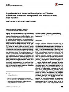
Figure 5. Simulated PBL heights along the west-to-east cross-section shown in Figure 1, at 1400 UTC (top panel) and 1800 UTC (bottom panel) on July 17.

however, predicted transitions from a deep mixing layer over land to a shallow layer over the Atlantic Ocean. However, the BLPBL generated a stronger sea breeze circulation than the GSPBL, as shown in Figures 4g and 4h, respectively. The larger sea breeze circulation predicted by the BLPBL is due to the more efficient vertical transport of heat flux over land, which creates a larger land-sea contrast above the surface. Figure 5 shows the PBL heights predicted by the two PBL schemes at 1400 UTC (top panel) and 1800 UTC (bottom panel) along the west-to-east cross-section through the 12-km domain, shown in Figure 1. It is clear that the PBL height diagnosed by the GSPBL scheme is systematically lower than that of the BLPBL scheme both during the morning and afternoon hours. The differences over land are about 300–500 m at 1400 UTC, and greater than 1000 m at 1800 UTC, east of about 81◦ W. The overall difference in PBL heights between the two models is about 50%. Also with the BLPBL scheme, the stability regime can change dramatically, as noted in the PBL collapse near 85.5◦ W, 78.8◦ W, and 75.2◦ W. This artificial collapse will be discussed in a later section. The reason for the substantially lower PBL height diagnosed by the GSPBL is that the predicted turbulence (TKE) cannot support a higher mixing layer. It is clear, then, that we need to determine whether convection or diffusion is better able to generate a more ‘realistic’ mixed layer.

BOUNDARY-LAYER EVOLUTION AND NOCTURNAL LOW-LEVEL JETS

185

Figure 6. Aircraft spiral measurements of (a) Tv ; (b) θv ; (c) RH; and (d) qv over PNE around 2000 UTC on July 17, and the corresponding BLPBL and GSPBL simulations.

Figures 6a–d show the profiles of virtual temperature (Tv ), θv , RH, and qv obtained from an aircraft spiral, and from MM5V3 at the grid cell that encompasses PNE around 2000 UTC on July 17. Several shallow inversions occurred between 1.7–2.2 km. A simple way to estimate the PBL height from the observations is to draw a vertical line from θv in the surface layer and find the intersection in the mixed-layer. The aircraft observations suggest that the mixed-layer height ranged from about 1.7 to 2 km. Although not shown here, profiles of O3 also suggest that the height of the PBL is near 2 km, but the estimates of PBL height will be slightly different when using profiles of different scalars. On the other hand, the modeldiagnosed PBL heights are 2.2 km by the BLPBL, and 1.1 km by the GSPBL. It is also obvious that even though the GSPBL predicted slightly higher temperature

186

K. ZHANG ET AL.

Figure 7. PBL heights predicted in the two original model simulations, compared with aircraft observations for 11 spirals over PNE and FME from July 17–19, 1999. The 1:1 line (dotted) is also shown. The error in observed PBL estimates, due to uncertainties in the height estimates and profiles of different scalars, is about 100–200 m. If a spiral nearly coincided with the top of an hour, only one PBL height is shown; otherwise, the range from one hour to the next is shown. The data points labeled ‘1’ (BLPBL) and ‘2’ (GSPBL) correspond to the model predictions shown in Figure 6.

fields at the surface, the GSPBL predicted lower T and θv (∼2 ◦ C) throughout the rest of the mixed-layer. In fact, although not shown here, a 1–2 ◦ C bias was observed at 2000 UTC along most of west-to-east cross-section, from about 86◦ W to the coastline (74◦ W). At the same time, the BLPBL overpredicted qv and RH above the well-mixed layer (>1.7 km). A significant feature in the observations is the sharp gradient in qv and RH at the top of mixed layer, but the model does not have sufficient vertical resolution (∼400 m) to resolve this feature near 1.7 km (see Table I). While Figures 6a–d compare the predicted and observed profiles at one time, Figure 7 compares the estimated PBL heights during 11 aircraft spirals from July 17–19 over PNE and FME. In Figure 7, when a spiral nearly corresponds to the top of an hour, the model-predicted PBL is shown; when a spiral occurred during an hour, the range in model-predicted PBL height is shown. In all cases, the observed PBL height has an uncertainty of about ±100–200 m, since the height of the spiral is estimated from the ambient pressure and assumes a standard atmosphere, and because profiles of different scalar quantities can suggest slightly different PBL heights. Except for five of the nighttime profiles (where the BLPBL scheme sets the PBL height to the lowest model level), the BLPBL may overestimate the PBL

BOUNDARY-LAYER EVOLUTION AND NOCTURNAL LOW-LEVEL JETS

187

Figure 8. Aircraft spiral, tethered balloon, and RASS profiler measurements of Tv around 2000 UTC on July 17.

height, while in general the GSPBL scheme tends to predict lower PBL heights. Given so few profiles during this period, this should be viewed as only a tentative assessment of the model’s ability to reproduce the observed PBL heights. Uncertainties exist not only in model simulations, but also among the different measurements. Figure 8 displays a typical Tv profile on July 17, suggesting that 1–2 ◦ C differences between the aircraft, tethered balloon, and RASS profiles are possible. As summarized by Angevine et al. [21], Tv measured by RASS is only accurate to about 0.5 ◦ C. Also, when the authors compared RASS to tower-based measurements, they found the mean bias and standard deviation of the biases to be about 1 ◦ C. These measurement uncertainties need to be taken into consideration when comparing model predictions with observations, as in Figures 6a–d and 7. 6.2. PBL EVOLUTION Figure 9 shows the time series of model-predicted PBL heights at the Baxter site from July 15–20. The GSPBL diagnosed the maximum PBL height to be about 1200 m during the first four days, about 800 m lower than that predicted by the BLPBL. In addition to the 30–40% difference in the PBL height, Figure 9 shows that the GSPBL predicted a slower growth rate for the mixing layer and a PBL collapse time about 1–2 h later than the BLPBL. This is due to the generation and

188

K. ZHANG ET AL.

Figure 9. Time series of simulated PBL height by the BLPBL and GSPBL schemes at the Baxter site, from July 15–20. All 5-day time series and time-height cross-sections start at 1200 UTC on July 15 and end at 1100 UTC on July 20.

dissipation of TKE, and the fact that vertical mixing by layer-to-layer diffusion is slower than direct non-local mixing by convection. The thermal stability regimes of the PBL can change rapidly in the BLPBL, which determine when direct mixing takes place. Berman et al. [22] showed that the maximum mixing height at New Brunswick, NJ during the July 13–15, 1995 episode ranged from about 1400– 2200 m, using meteorological fields from a similar MM5 simulation (with the BLPBL) scheme and from two sets of independent observations – sonde-based Tv , and profiler-based refractive index structure parameter (Cn2 ) measurements. The authors determined that the BLPBL was able to simulate both the morning growth rate and the height of the PBL quite well during this episode. Using a different set of independent observations for model comparison, and considering a different synoptic situation (mid-July 1999), our results also suggest that the mixing processes of the BLPBL are able to simulate the behavior of the convective PBL rather well. On the timescales of vertical mixing processes ( 0). In the original BLPBL scheme, the stable regimes were classified according to surface parameters alone. There are certainly times when a stable surface layer is indicative of a stable PBL as a whole. However, this classification may not reflect the potential of the PBL as a whole to support convection. Surface stability alone is not sufficient to characterize the potential for convection over the entire PBL, such as when there is positive convective energy above a stable surface layer. With this modification, the PBL heights over land are more reasonably diagnosed, and the sudden collapse of the PBL in isolated areas is eliminated. The second modification, mentioned previously, is the exclusion of FDDA from the lower atmosphere. In this modification, FDDA is only applied to the atmosphere above the diagnosed PBL height or the lowest 8 model layers (∼1.3 km), whichever is higher, since the jet core occurs near 400–700 m and the effects of the jet extend to about 1 km. Hence, the lower atmosphere is always free from nudging, both during the daytime and nighttime. This approach is similar to the work by Shafran et al. [2], who limited FDDA to above 1.5 km, leading to the improved simulation of the low-level wind fields, and possibly limiting the daytime development of the PBL. With the above modifications to MM5V3, the new experiments, denoted as the MBLPBL and MGSPBL simulations, were carried out for same period. Figures 13d and 13e show the wind speeds, and Figures 14d and 14e show the wind directions simulated by the MBLPBL and MGSPBL, respectively. Note that in the modified simulations, the maximum wind speeds in the vicinity of the jet during the nights of July 16–18 increased to about 10 m s−1 . The improvement in the

194

K. ZHANG ET AL.

strength of the LLJs is substantial; while the original MM5V3 predicted jet core maxima which are about 50% as high as the observations, the modified MM5V3 is able to predict jet core maxima that are about 75–90% of the observed wind speeds. The modified PBL simulations, therefore, have better simulated the LLJ strength, especially on July 16. Although the modifications led to higher wind speeds, the model was still not able to reproduce the sharp vertical gradients near 400 m since the vertical resolution was kept the same, and because of the weak nocturnal turbulence. The BLPBL and MBLPBL simulations both predicted winds speeds higher than observed extending to the surface, while the MGSPBL scheme predicted large wind speeds (>6 m s−1 ) only above about 100 m. The most significant improvement occurs in the timing of the LLJs. Because the modified simulations are free from FDDA below 1.3 km, the low-level wind fields are controlled by the intrinsic dynamics. The simulated LLJs now reach their maxima at 0600, 0300 and 0600 UTC in the MBLPBL experiment, and at 0700, 0100 and 0800 UTC in the MGSPBL experiment on July 16–18, respectively. These timings of occurrence of the maximum LLJs are closer to the observations than the 0000 UTC predicted by the original experiments (Figures 13b and c). The time-height cross-sections of the modified wind directions are displayed in Figures 14d and 14e, while the time series of the wind direction and speed at 654 m are shown in Figures 15a and 15b. During the daytime hours, southwesterly flows were predicted by both modified simulations, extending to about 1 km; however, westerly flow near the surface on July 17 was not captured well by the modified simulations. During the morning hours, westerly flow dominated the observed wind near 654 m. The wind direction suddenly changed to southwesterly between 1800– 2100 UTC, due to upward mixing of momentum. During the nighttime, the wind direction slowly changed to westerly with increasing wind speeds, reflecting a decoupling of the LLJ and the surface layer. This diurnal pattern occurred on each of the first four days before a cold front arrived on the last day. All simulations were generally able to model the diurnal cycle, but tended to lead observations by a few hours during the daytime as the wind direction changed from westerly to southwesterly. The best agreement between observations and simulations occurs during nighttime hours when the LLJs develop. 7.4. HORIZONTAL SCALE AND VERTICAL STRUCTURE OF THE LLJS The model simulations can be used to examine the horizontal and vertical scales of the LLJs. Figures 16a–d show the simulated wind fields near the jet core height of 950 mb (654 m) at the time of peak wind speeds (0400 UTC) on July 17 (see Figure 12b). With FDDA, both the BLPBL and GSPBL generated similar wind fields; along the northeastern U.S. seaboard, the largest wind speeds (>10 m s−1 ) occurred over Long Island and over the Atlantic Ocean off the coast of CT in both the BLPBL (Figure 16a) and GSPBL (Figure 16b) simulations. The situation is rather different in the MBLPBL (Figure 16c) and MGSPBL (Figure 16d) simula-

BOUNDARY-LAYER EVOLUTION AND NOCTURNAL LOW-LEVEL JETS

195

Figure 12. Hourly wind profiler observations at the Baxter site on (a) July 16; (b) July 17; and (c) July 18.

tions without FDDA. Horizontally, the simulated LLJs are more than 200 km wide. The MBLPBL simulation predicted maximum wind speeds near Boston, MA of 18 m s−1 , while the MGSPBL predicted a large region from NY to MA having wind speeds greater than 18 m s−1 , with a 20 m s−1 center over CT. Since the RASS profiler at Stow, MA did not detect such high wind speeds, it appears that

196

K. ZHANG ET AL.

Figure 13. Time-height cross-sections of wind speed at the Baxter site from July 15–20: (a) wind profiler observations; (b) BLPBL; (c) GSPBL; (d) MBLPBL; and (e) MGSPBL.

Figure 14. Same as Figures 13a–e, except for wind direction.

BOUNDARY-LAYER EVOLUTION AND NOCTURNAL LOW-LEVEL JETS

197

Figure 15. Time series of (a) wind direction and (b) wind speed at the Baxter site from July 15–19, at about 654 m (near the jet core), from the observations and the original and modified simulations.

the modified simulations actually overpredicted the jet intensity at this time. This may be due to the underestimation of nighttime turbulence. The vertical structure of the LLJs along the New Jersey cross-section, simulated in the four experiments, is displayed in Figures 17a-d. The BLPBL (Figure 17a) and GSPBL (Figure 17b) predicted LLJs with wind speed below 10 m s−1 , which are weaker than the RASS observations. The simulated heights of the jet cores are too low, only at about 100–200 m by the GSPBL and 200–300 m by the BLPBL. The BLSPBL (Figure 17c) and GSLPBL (Figure 17d) predicted stronger LLJs on the order of 12–14 m s−1 , which are comparable to RASS observations at the Baxter site. The height of the jet core increases from about 200 m over the ocean to about 300 m over land in the MGSPBL, still too low compared to the 400–600 m level seen in the observations. The centers of the MBLPBL-simulated LLJs are

198

K. ZHANG ET AL.

Figure 16. Simulated wind fields near the height of jet core (654 m) at 0400 UTC on July 17 by (a) BLPBL; (b) GSPBL; (c) MBLPBL; and (d) MGSPBL. Wind speed is shown in 2 m s−1 contour intervals.

located at 400 m over the ocean and about 600 m over land, in better agreement with the observations. All of these model differences and uncertainties will affect air quality simulations in a non-linear fashion. This is important since, as noted before, pollutants trapped aloft in the residual layer are transported over large distances by the LLJs during the night. Differences in wind speed and direction will lead to different PBL ventilation and pollutant transport directions. 8. Statistical Evaluation of the Surface Level and Vertical Structure of PBL 8.1. SURFACE LEVEL To summarize the overall performance of the MM5V3 simulations, we compared the hourly observed and predicted temperature, specific humidity, wind speed, and wind directions at the surface from the July 15–20 period. The statistics include the mean and standard deviation of the differences (defined as ‘model prediction minus observation’), root mean square error (RMSE), index of agreement, systematic error, and unsystematic error [33]. The data were also separated by ‘daytime’ hours (1200–0000 UTC) and ‘nighttime’ hours (0000–1200 UTC).

BOUNDARY-LAYER EVOLUTION AND NOCTURNAL LOW-LEVEL JETS

199

Figure 17. Simulated wind speeds along the New Jersey cross-section at 0400 UTC on July 17: (a) BLPBL; (b) GSPBL; (c) MBLPBL; and (d) MGSPBL. The Atlantic coastline is located near the middle of each panel.

200

K. ZHANG ET AL.

Table III. Basic statistics for the hourly surface temperature observations and MM5V3 predictions during the July 15–20, 1999 period: (a) daytime hours, 1200–0000 UTC, and (b) nighttime hours, 0000–1200 UTC. The statistics shown are the mean difference, standard deviation (σ ) of the difference, root mean square error (RMSE), index of agreement, systematic error, and unsystematic error. Differences are calculated as ‘model prediction minus observation’. Simulation

Mean difference ( ◦ C)

σ of difference ( ◦ C)

RMSE ( ◦ C)

Index of agreement (%)

Systematic Unerror systematic (%) error (%)

1.7 1.7 1.8 1.7

94 94 94 94

10 4 15 3

90 96 85 97

1.7 1.8 1.5 1.6

91 91 92 92

30 31 15 26

70 69 85 74

(a) Daytime, 1200–0000 UTC BLPBL GSPBL MBLPBL MGSPBL

−0.3 0.1 −0.7 −0.3

1.7 1.7 1.6 1.7

(b) Nighttime, 0000–1200 UTC BLPBL GSPBL MBLPBL MGSPBL

0.9 1.0 0.6 0.8

1.5 1.5 1.4 1.4

The temperature statistics are shown in Table III. During the daytime, the BLPBL and modified PBL simulations on average have negative biases, while the GSPBL predicted a slight positive bias. In terms of the spread of the differences between the model and observations, the original and modified simulations had very similar standard deviations and RMSE values. In all cases, the unsystematic errors were substantially higher than the systematic errors. During the nighttime hours, where the effects of FDDA are pronounced, the biases were positive and larger than during the daytime. The systematic errors were also larger at nighttime than during the day. Table IV shows the statistics for the specific humidity. The results are similar to temperature, in that the mean bias, standard deviation, and the RMSE were similar in all of the PBL simulations. The fact that the differences between the original and modified simulations for temperature and humidity are not substantial is not unexpected, since the modified FDDA scheme was used to improve the simulation of the vertical wind field structure (i.e., LLJs). The situation with wind speed and direction is somewhat different (see Table V for wind speed and Table VI for wind direction). During the day, when surface wind speeds are low, there are substantial differences (∼55–60 deg) between the observations and predictions; the removal of FDDA greatly reduces these biases at

201

BOUNDARY-LAYER EVOLUTION AND NOCTURNAL LOW-LEVEL JETS

Table IV. Same as Table III, except for specific humidity. Simulation

Mean difference (g kg−1 )

σ of difference (g kg−1 )

RMSE (g kg−1 )

Index of agreement (%)

Systematic Unerror systematic (%) error (%)

1.6 2.5 1.8 2.4

82 70 81 71

25 65 37 64

75 35 63 36

1.8 1.9 1.9 2.0

80 78 78 76

51 61 59 65

49 39 41 35

(a) Daytime, 1200–0000 UTC BLPBL GSPBL MBLPBL MGSPBL

0.8 2.0 1.0 1.9

1.4 1.5 1.4 1.5

(b) Nighttime, 0000–1200 UTC BLPBL GSPBL MBLPBL MGSPBL

1.2 1.5 1.5 1.6

1.2 1.2 1.2 1.2

Table V. Same as Table III, except for wind speed. Simulation

Mean difference (m s−1 )

σ of difference (m s−1 )

RMSE (m s−1 )

Index of agreement (%)

Systematic Unerror (%) systematic error (%)

4.4 5.1 4.2 4.9

51 42 57 45

55 65 47 61

45 35 53 39

2.9 3.0 2.7 2.9

56 53 63 57

18 23 4 18

82 88 96 82

(a) Daytime, 1200–0000 UTC BLPBL GSPBL MBLPBL MGSPBL

−3.3 −4.1 −2.8 −3.8

3.0 3.1 3.1 3.1

(b) Nighttime, 0000–1200 UTC BLPBL GSPBL MBLPBL MGSPBL

−1.0 −1.3 −0.5 −1.1

2.6 2.7 2.7 2.7

202

K. ZHANG ET AL.

Table VI. Same as Table III, except for wind direction. Negative wind direction biases indicate that on average, the model-predicted wind direction is rotated counterclockwise with respect to the observed wind direction. Simulation

Mean difference (degrees)

σ of difference (degrees)

RMSE (degrees)

Index of agreement (%)

Systematic Unerror (%) systematic error (%)

161 162 159 160

50 50 52 50

12 12 13 13

88 88 87 87

106 105 107 108

73 72 74 73

17 18 19 19

83 82 81 81

(a) Daytime, 1200–0000 UTC BLPBL GSPBL MBLPBL MGSPBL

−59 −57 −59 −58

149 151 148 150

(b) Nighttime, 0000–1200 UTC BLPBL GSPBL MBLPBL MGSPBL

−40 −41 −38 −40

98 97 100 99

night. Also, the unsystematic error at night is much larger than during the daytime. For wind direction, the day–night differences are also larger than the differences across the four simulations. This is not unexpected, since the effects of FDDA are largest at night, and frictional losses at the surface are the same in all simulations. 8.2. UPPER LEVELS It is anticipated that the largest differences simulated by the two PBL schemes should occur in the vertical, since all simulations use common air-land interaction schemes and the same synoptic surface analyses in the FDDA fields. In this section, we attempt to quantify the differences between the observations and simulations by examining the mean and standard deviation of the biases, in the vertical. The observations are hourly-averaged RASS and wind profiles from July 15–19, 1999 from the Baxter site. All observations were averaged within the appropriate model layers (Table I) in order to compare with simulations; the observation levels were not interpolated to match the MM5 levels. The vertical extent is limited by the availability of observations. We did not include data from July 20 because of the passage of a cold front on that day. Bias statistics were generated for daytime (1200–0000 UTC) and nighttime (0000–1200 UTC) hours separately in order to identify the strengths and weaknesses of the schemes for each PBL regime. Although the biases above 1 km are displayed in the following figure, the limited

BOUNDARY-LAYER EVOLUTION AND NOCTURNAL LOW-LEVEL JETS

203

availability of observed data causes the largest biases to occur at this height; hence, we focus on comparisons below 1 km. Figure 18 shows the observed mean profiles of daytime Tv and nighttime wind speed and direction, and the corresponding model biases at the Baxter site. The observations are shown on the left-most column. The respective biases of the BLPBL, GSPBL, MBLPBL, and MGSPBL are shown in columns 2–5, respectively. Note that the Tv observations are characterized as having an average daytime lapse rate of about 7 ◦ C km−1 . The overall errors are small, with temperature biases less than 2 ◦ C, except for the MGSPBL above 1 km. A systematic difference in the daytime bias profile occurs below 1 km: the BLPBL and MBLPBL are slightly positively biased (