The present work provides a numerical method for the simulation of wet-steam flows with polydispersed spectra. The so-called moment method is used to ...
Numerical Method for Wet-Steam Flows with Polydispersed Droplet Spectra Michele Giordano∗ and Paola Cinnella† Universit` a del Salento, Lecce, 73100, Italy The present work provides a numerical method for the simulation of wet-steam flows with polydispersed spectra. The so-called moment method is used to represent the liquid droplet evolution. This approach is based on a partial modeling of the droplet size distribution, through the resolution of transport equations for the lowest-order moments of the droplet spectrum, which allows evaluating the wetness fraction and the mean radius of the droplets. These transport equations are coupled with the Euler equations that govern the motion of the two-phase mixture. Several equations of state are adopted to model the thermodynamic behavior of the vapor phase. The system of the governing equations is solved through an uncoupled procedure: the main equations for the mixture are solved first, then the main flow properties are frozen and used to solve the additional equations. All of the equations are discretized by means of a third-order accurate centered scheme.
I.
Introduction
large number of research areas are concerned with the modelling and simulation of steam flow. Relevant A applications are aircraft flight in humid air conditions, wet-steam flows in turbines and droplet-spray combustion processes. In particular, for low pressure (LP) turbines great attention has to be paid to the condensation phenomena, responsible of blade erosion and losses in turbine efficiency. The wet-steam flow is usually modelled as a gas-droplet multiphase flow in which coexistence between vapor and liquid droplets exists.1 Spontaneous nucleation leads to the formation of liquid droplets from vapor. A key point in the computation of these flows as many other two-phase phenomena is the determination of the shape of the droplet spectrum. For instance, droplet deposition onto steam turbine blades is extremely sensitive to droplet size. Even if there are two-phase cases which do not require the entire droplet distribution, modelling the liquid phase by means of a single, averaged droplet size generally results in incorrect coupling between the liquid and the vapor phases. Different approaches are available in the literature for wet-steam modeling. They mainly divide into those which treat the full spectrum of sizes of liquid droplets, and those which try to model only part of it. The former category further sub-divides into the mixed Eulerian-Lagrangian and the fully Eulerian approaches. At date, probably, the most followed one is the mixed Eulerian-Lagrangian,2–4 where conservation equations for the two-phase mixture are solved in an Eulerian reference frame, while nucleation and droplet growth are computed following fluid particles (Lagrangian approach). A possible reason for the mixed model success lays in the chance of being less prone to numerical errors within a Lagrangian framework, especially for steady flow with no velocity slip. On the other hand the full Eulerian approach3, 5 provides better opportunities for extensions to unsteady flows and to flows with slip. Other models rather try to partly reproduce the droplet size distribution. The moment approach3, 6–8 correctly model exchanges of heat and mass between the phases, but involves less computation than discrete spectrum calculations, since models only the first few moments of size distribution. This is the main reason which leads us to the choice of this approach to simulate the vapor-droplet mixture. One of the most attractive, among the several possible applications, of this approach is represented by the simulation of two-phase flow turbines, generally used for electric power generation from renewable sources such as geothermal and solar sources, and for cogeneration. At this time, the efficiencies of existing two-phase ∗ Post-Doc † Assistant
Researcher, Dipartimento di Ingegneria dell’Innovazione, Via per Monteroni, 73100, Lecce, Italy. Professor, Dipartimento di Ingegneria dell’Innovazione, Via per Monteroni, 73100, Lecce, Italy, AIAA Member.
1 of 16 American Institute of Aeronautics and Astronautics
turbines are poor, since no proper optimization of their shapes is performed. Then, the aim of this work is the realization of a numerical methodology able to simulate those turbines, in order to study in detail different existing types of two-phase turbines and to identify the main loss mechanisms. The new insights provided by the study will allow to propose suitably modified turbine, with increased performances in terms of efficiency and durability. In the following the moment method is described, along with the numerical approach proposed for the solution of the resulting governing equations. Validation results are discussed, and final conclusions are drawn.
II.
The Moment Method
This approach,3, 6–8 as stated in the introduction, is based on the assumption that the full droplet spectrum in not required in most cases. In such cases, the correct coupling between vapor and liquid droplets is achieved just computing the first few moments of the size distribution. A.
Mixture Conservation Equations
Conservation equations for the two-phase mixture take the same form of their single phase counterparts. For inviscid, adiabatic wet-steam flow with no inter-phase slip, the mass continuity , momentum and energy equations for the two-phase mixture in conservation variables are ∂ ρm + ∇ · (ρm u) = 0 , ∂t
(1)
∂ (ρm u) + ∇ · (ρm u u) + ∇p = 0 ∂t
,
(2)
∂ (ρm E) + ∇ · (ρm E u) + ∇ · (pu) = 0 , (3) ∂t where u represents the common velocity field, ρm is the mixture density and E is the mixture total energy per unit mass. Their definitions are 1−y y 1−y 1 = + ≃ ρm ρv ρl ρv 1 E = e + u2 , 2 e = (1 − y) ev + y el
,
(4) (5)
,
(6)
with e equal to the internal energy per unit mass of the mixture. The subscripts m, v and l referred to mixture, vapor and liquid, respectively. The relation between mixture total energy E and total enthalpy H, both per unit mass, is given from H =E+
p ρm
,
(7)
since H
= (1 − y) Hv + y Hl =
= (1 − y) (Ev + p/ρv ) + y (El + p/ρl ) =
= (1 − y) Ev + y El + p ((1 − y)/ρv + y/ρl ) =
= E + p/ρm B.
(8)
.
Droplet Conservation Equations
The droplet size distribution varies continuously in time and space, and is described by the droplet number density function f . Thus, f dr represents the number of droplets per unit mass of mixture in the size range r to (r + dr).
2 of 16 American Institute of Aeronautics and Astronautics
If we introduce a 3D particle phase space (Fig.1) composed of two spatial dimensions, x and y, and a particle size dimension, r, given the control volume dV ′ , the total number of droplets NV contained in dV ′ is Z NV = ρm f dV ′ . (9) Note that dV ′ is defined as the elemental volume in the given frame, and it is equal to dV ′ = dx dy dr.
r
y dS’
x Figure 1. Moment method - control volume in the “particle phase space”.
The trajectories of droplets in phase space are described by the phase velocities, with the usual velocity components plus a droplet growth velocity: ux dx/ dt u′ = dy/ dt = uy , (10) dr/ dt G or referring to u as the usual velocity components:
u G
′
u =
!
.
(11)
Starting from definition (9), an expression for the droplet conservation in Eulerian form is derived. First, we assume no droplet breakup or agglomeration, so that changes in NV are due only to nucleation of new droplets within the control volume and to fluxes through the control surface. Those fluxes include the usual convective fluxes plus an additional droplet growth flux. The droplet conservation equation is thus Z I Z ∂ ρm f dV ′ + ρm f u′ · dS′ = ρm J dV ′ , (12) ∂t where J is the nucleation rate and dS′ the surface control area of dV ′ . The equation, written in differential form, reads as ∂ (ρm f ) + ∇′ · (ρm f u′ ) = ρm J ∂t where ∇′ is given by
∂/∂x ∇′ = ∂/∂y ∂/∂r
,
.
3 of 16 American Institute of Aeronautics and Astronautics
(13)
(14)
Expanding equation (13), and reverting it to the familiar physical space, we obtain ∂ ∂ (ρm f ) + ∇ · (ρm f u) + (ρm f G) = ρm J ∂t ∂r
,
(15)
where r is the particle size dimension and G = dr/ dt is the droplet growth rate. C.
Moment Equations
A relevant benefit coming from the use of the moments of the droplet size distribution is that vapor-liquid heat and mass transfer can be accurately modelled by solving a few moment equations, rather than a larger number related to numerous droplet groups. The jth moment of the droplet size distribution is defined as Z ∞ µj = rj f dr . (16) 0
Low order moments have a physical significance. In particular, µ0 is equal to the total number of droplets per unit mass of mixture and µ3 is proportional to the wetness fraction µ0 = nT µ3 =
3 y 4πρl
,
(17) .
(18)
So in order to determine y, an equation describing the evolution of µj is needed. This is done multiplying Eq. (15) by rj and integrating over all radii. Adopting integration by parts for the last term in the LHS, and noting that rj f vanishes at r = 0 and r = ∞, we have Z ∞ ∂ (ρm µj ) + ∇ · (ρm µj u) = jρm rj−1 Gf dr + ρm J∗ r∗j . (19) ∂t 0 It is assumed that droplets form only at a critical radius r∗ , so that the nucleation rate can be written as Dirac-delta function J = J∗ δ(r − r∗ ) , (20) with J∗ and r∗ defined below. Once µ3 is determined, and so y, it is possible to proceed to the computation of the mixture conservation equations, and, so, no further moment equations need to be solved. D.
Further Details on the Model
Further details are given, mainly regarding the definitions of the critical radius, the nucleation and the droplet growth rates. 1.
Critical Radius
Following the definition from Kelvin-Helmholtz, the critical radius r∗ is given by r∗ =
2σ Ts (p) 2σ ≈ ρl RTv ln S ρl hvl ∆T
,
(21)
with σ the surface tension, Ts (p) the saturation temperature at pressure p, hvl = hv − hl the specific enthalpy of evaporation and ∆T = Ts (p) − Tv the vapour subcooling. S is the supersaturation ratio and is given by S=
p ps (Tv )
,
with ps (Tv ) being the saturation pressure at temperature Tv .
4 of 16 American Institute of Aeronautics and Astronautics
(22)
2.
Nucleation Rate
The rate of nucleation is calculated from classical theory, modified to include non-isothermal effects8, 9 r � � 4πr∗2 σ qc ρv 2σ J∗ = , (23) exp − 1 + θ ρl πm3 3kTv where qc is the condensation coefficient, usually taken equal unity, m the mass of a single molecule and k is Boltzmann’s constant. The nonisothermal correction factor θ is equal to � � hvl 2(γ − 1) hvl θ= − 0.5 . (24) 1 + γ RTv RTv 3.
Droplet Growth Rate
Following a modified form of Gyamarthy’s formula, the growth rate is given by10, 11 G=
kv ∆T (1 − r∗ /r) ρl hvl (r + 1.89(1 − ν)λv /P rv )
,
(25)
with P rv the Prandtl number of the vapour, kv the vapour thermal conductivity and λv the mean free path of a vapour molecule, defined as √ 1.5µv RTv λv = , (26) p where µg is the vapour dynamic viscosity. The parameter ν is given by � � RTs (p) 2 − qc γ + 1 RTs (p) ν= β − 0.5 − hvl 2qc 2(γ − 1) hvl
,
(27)
where β is an empirical parameter, which typically takes values between 0 and 5. E.
Closure of Moment Equations
The closure of the moment equations strictly depends on the representation of the droplet growth rate G. If a linear relation is adopted, as G = a0 + a1 r , (28) the integral in equation (19) is replaced by a linear combination of µj and µj−1 . Here, the droplet growth is approximated by a constant growth rate: G = a0
with
a0 = G(r20 ) ,
(29)
where r20 is the local surface-averaged radius given by r20 = (µ2 /µ0 )1/2
.
(30)
The reason behind this solution sides in the need of a more robust implementation, even if less accurate in the transient. Note that for µ0 , whatever is the choice for G, the integral at the RHS of equation (19) vanishes since j = 0.
III.
Thermodynamic Model
Several equations of state (EOS) are adopted to represent the vapor phase thermodynamic behaviour. In this section they are shown together with the corresponding caloric equations.
5 of 16 American Institute of Aeronautics and Astronautics
A.
Perfect Gas Equation
The standard EOS for perfect polytropic gases is adopted for the vapor as pvv = Rv Tv
,
(31)
ev = cv∞ ,v Tv
,
(32)
and it is coupled with the caloric equation
where cv∞ ,v is the ideal-gas-limit specific heat capacity at constant volume referred to the vapor. B.
Van der Waals Equation
The van der Waals equation for the vapor phase is p=
Rv Tv α − 2 vv − β vv
where α and β are two gas dependent parameters. The caloric equation has to be computed from "
dev = cv∞ ,v dTv + Tv
�
∂p ∂Tv
,
�
vv
(33)
#
− p dvv
,
(34)
and, since we adopt a constant value for cv∞ ,v , we obtain ev = cv∞ ,v Tv − C.
α vv
.
(35)
pvv = Rv Tv (1 + Z) ,
(36)
Z Equation
The Z-factor equation of state
10, 11
is given by
where the factor Z is equal to Z = a Tvb pc
,
(37)
and a = −1.439 · 106 , b = −5.2 , c = 1.08 .
(38)
This time, the caloric equation is computed from "
dhv = cp∞ ,v dTv + vv − Tv
�
∂vv ∂Tv
� #
dp
,
(39)
p
where cp∞ ,v is the ideal-gas-limit specific heat capacity at constant pressure referred to vapor. By adopting a constant value for cp∞ ,v , we obtain hv = cp∞ ,v Tv −
b Rv T v Z a b Rv T b+1 pc = cp∞ ,v Tv − c c
and in term of specific energy ev = cp∞ ,v Tv −
p b Rv T v Z − c ρv
.
6 of 16 American Institute of Aeronautics and Astronautics
,
(40)
(41)
IV.
Implementation and Numerical Details
In this section full details on the implementation and on the numerical approach are given. In particular, the equation used to compute pressure and temperature starting from the mixture specific energy and the modifications adopted to deal with quasi-1D flow are recalled. Then, the implicit treatment of the source terms in the moment transport equations is discussed and the spatial discretization scheme used to approximate the convective terms is described. A.
Pressure and Temperature Computations
In order to compute pressure and temperature from the mixture specific energy coming from the solution of the mixture Euler equations, some algebric manipulations are needed: e = (1 − y) ev + y el =
= ev + y (el − ev ) = � � = ev + y hl − hv − ρpl + ρpv = � � = ev + y ρpv − ρpl − hvl ,
(42)
where ev is given by the caloric equation of state and the evaporation latent heat hvl is a function of the vapor temperature Tv (see Appendix A). Regarding ρl , we used a constant value, but a function of Tv can be used for more accurate calculations. Coupling equation (42) with the thermal and caloric equations of state, it is then possible to directly compute pressure and temperature from the mixture specific energy e. B.
Quasi-1D Flow
In this paper only quasi-1D computations are performed. In this case, the velocity field u reduces to the scalar field u. Due to the area variation, typical of quasi-1D flow, respect to the Euler equations (1-3), a source term has to be introduced on the right-hand side of the equations: ρm u dA − A(x) SA1 dx 2 m u dA , SA = SA2 = (43) − ρA(x) dx ρm u E+p u dA SA3 − A(x) dx where A(x) is the area, dA/dx its variation. Similarly, a source term has also to be introduced on the right-hand side of the transport equations (19): ρm u µo dA − A(x) dx STA1 u µ1 dA − ρm STA2 A(x) dx STA = . (44) = ρ m u µ2 dA STA3 − A(x) dx STA4 − ρm u µ3 dA A(x)
C.
dx
Treatment of the Source Terms
In this section we spent a few words about the treatment of the source terms in the moment transport equations. This set of equation is characterized by considerable stiffness, since each moment has a magnitude much bigger than the moments of lower order, and the moment transport equations contain stiff source terms related to droplet nucleation and growth. While the nucleation rate is always positive, the contribution coming from the growth rate (25) can be either negative or positive in the transient. So, it comes out the need to treat implicitly this term. In this work, a semi-implicit approach is adopted, which means that the growth rate is treated implicitly only when it is negative and stability problems may arise. Referring to a generic differential equation in the variable φ dφ = S(φ) φ dt
,
7 of 16 American Institute of Aeronautics and Astronautics
(45)
where S(φ) represents the non-linear source term, it is discretized as follows ∆φ = S(φn ) φn + S − (φn ) ∆φn ∆t
,
(46)
where
S(φ) − |S(φ)| , (47) 2 and S − is zero if S is positive and is equal to S if S is negative. Then, an implicit scheme is applied when the source term is negative, an explicit scheme is applied otherwise. S − (φ) =
D.
Numerical Details
The governing equations are discretized using a cell-centred finite volume scheme of third-order accuracy, extended to the computation of flows with an arbitrary equation of state.12 The scheme is constructed by correcting the dispersive error term of second-order-accurate Jameson’s scheme.13 The use of a scalar dissipation term simplifies the scheme implementation with highly complex equations of state and greatly reduces computational costs. The governing equations are integrated in time using a four-stage Runge–Kutta scheme. Local time-stepping is used to efficiently drive the solution to the steady state. In previous works, the method has been successfully validated for a variety of single-phase flows of perfect and real gases (see 12, 14, 15 and references cited therein). The main set of the Euler equations for the two-phase mixture (1-3) and the auxiliary set of transport equations (represented by the j th equation (19)) for the droplet distribution spectra are solved by means of an uncoupled procedure: at each time step the properties of the mixture are first computed by solving the main equations with frozen droplet properties; then the auxiliary equation are solved by using the frozen mixture properties. Because of mechanical equilibrium, the pressure field is supposed to be the same for both phases (surface tension is neglected).
V.
Supersonic Nozzle
The proposed model and numerical approach validated for wet-steam flows in a nozzle, for which numerical results and experimental data are available in the literature.3 Then, the effects of the adopted models for the equations of state and for the droplet evolution equations are shown. Let as consider a quasi-1D nozzle, with inlet conditions corresponding to a total pressure p0 = 0.25 bar and total temperature T0 = 358 K. The simulation is performed from the throat to the exit of the nozzle, imposing sonic condition at the inlet. The geometry of the nozzle is given in Appendix B. The computations have been performed by using a uniform grid composed by 400 cells. Figure 2 displays a comparison of the static pressure distribution along the nozzle (normalized with inlet total pressure) with numerical and experimental data taken from Ref. 3. The present solution has been obtained using the Z equation of state, which is the same adopted for the numerical calculations of Ref. 3. Note that in Ref. 3 the governing equations for the fluid mixture and for the moment transport equations are discretized by using the second-order Jameson scheme, and the cp∞ ,v is not constant but a function of Tv . Moreover, the droplet growth rate is not approximated by a constant rate as in the present work, but by a three-term function of the mean droplet radius. In particular, two numerical solutions are reported from the given reference: one related as Literature-Moments where the simulation is performed which an approach very similar to the present (i.e. the moment method); another one related as Literature-Euler where the simulation is made adopting an Eulerian-Eulerian approach for the vapor and the liquid phases. The present results are in quite good agreement with experimental data, and the solution appears to be more accurate than that of Ref. 3 obtained by the moment method, and substantially similar to the more expensive one obtained by the Eulerian approach. Figure 3) shows the distributions of the mean droplet diameter (computed as r10 = µ1 /µ0 ) along the nozzle corresponding to the present calculations and compares it to the numerical results and experimental data of Ref. 3. In this case, we obtain lower values of the droplet diameter compared both to previous numerical results and to experimental data. In particular, the present results underestimate the mean droplet diameter of about 40%, whereas results in Ref. 3 for the moment method provide a value which is 20% closer to the experimental one. The Eulerian computation stands in the middle. A possible reason for this major
8 of 16 American Institute of Aeronautics and Astronautics
underestimation could be found in the more accurate representations of the cp∞ ,v and of the droplet growth rate in,3 but it is still under investigation. In Figures 4 and 6 the solutions for the pressure and the droplet diameter along the nozzle are shown for the different equations of state: all the three EOS results very similar for the obtained results, and this is probably due to the fact that for the given pressure and temperature the vapor behaves as a perfect gas. However, the Z equation is probably the closer to the experimental data, since presents a less premature pressure rise (see Figure 5). Note that in Fig. 4 the solution for a dry steam (i.e. without liquid droplet nucleation) is also reported. This one, compared with the other simulations of wet-steam flow, let us understand the effects of the liquid droplet formation. At about x = 0.1 the pressure presents a rise due to the starting of the nucleation, and then it decreases as expected in a supersonic diffuser. This phenomenon causes an higher level of the static pressure at the exit of the nozzle, respect to the dry steam calculation. If we look at Figure 7, where the temperature-total temperature ratio along the nozzle is shown, again the nucleation of liquid droplets causes a rise in the temperature and then it decreases, even reaching an higher value at the exit of the nozzle respect to the dry steam computation. Four droplet parameters are shown in Figures 8-9: the wetness fraction, the supersaturation ratio, the number of droplets and the nucleation rate, the last two respectively scaled by 1019 and 1021 . Note that as expected the nucleation rate has the maximum just before x = 0.1 causing the rise in pressure and temperature. Then, in Fig. 9 it is possible to appreciate also the dependency of the nucleation rate from the supersaturation ratio. They present the maximum value in the same point since when the supersaturation ratio reaches its maximum the critical radius has its minimum value, and at this time nucleation can begin, i.e. when the droplet radius is greater than the critical radius.
0.55 Present - Z Equation Literature - Experiment Literature - Moments Literature - Euler
0.5
p / p0
0.45
0.4
0.35
0.3
0.25
0
0.1
0.2
0.3
0.4
X Figure 2. Pressure ratio - comparison between the present solution with the Z equation and experimental and numerical data coming from3 for the pressure.
9 of 16 American Institute of Aeronautics and Astronautics
Present - Z Equation Literature - Experiment Literature - Moments Literature - Euler
Droplet Diameter (microns)
0.1
0.08
0.06
0.04
0.02 0
0.1
0.2
0.3
0.4
X Figure 3. Droplet diameter - comparison between the present solution with the Z equation and experimental and numerical data coming from3 for the pressure.
0.55
+ + + 0.5 + + + + 0.45 + +
+
p / p0
+
0.4
+ +
+
+ + +
+
+ +
+
+
+
0.35
+
Present - PG Equation Present - VdW Equation Present - Z Equation Present - Dry Steam
+
0.3
+
+
+
+
+
+
+
+
+ + + +
0.25
0.2
0
0.1
0.2
0.3
0.4
X Figure 4. Pressure ratio - comparison between the solutions from the different equations of state and the dry steam.
10 of 16 American Institute of Aeronautics and Astronautics
0.4 +
+ + +
+ +
+
+
+
+
+
0.39
+
+
+ +
+
+
p / p0
+
+ +
+
0.38
+ +
+
+
+
+ +
+
+
+
+
Present - PG Equation Present - VdW Equation Present - Z Equation
+
0.37 + + +
0.36 0.1
+
+ + + + +
0.12
0.14
0.16
0.18
0.2
X Figure 5. Pressure ratio - zoomed area for the comparison between the different equations of state adopted.
0.1
Droplet Diameter (microns)
+
Present - PG Equation Present - VdW Equation Present - Z Equation
0.08
0.06 +
+
+ + + + + + + + + + + + + + +
+ + + + + + + +
0.04
0.02 +
0
0.1
0.2
0.3
0.4
X Figure 6. Droplet diameter - comparison between the solutions from the different equations of state.
11 of 16 American Institute of Aeronautics and Astronautics
T / T0
0.88 + + + + + + 0.84 + + + + + + + + + + 0.8 + + + + +
+ + + + + + + + + + + + + + + +
+
Present - PG Equation Present - VdW Equation Present - Z Equation Present - Dry Steam
0.76
0.72
0.68 0
0.1
0.2
0.3
0.4
X Figure 7. Temperature ratio - comparison between the solutions from the different equations of state and the dry steam.
0.05
+
Present - PG Equation Present - VdW Equation Present - Z Equation
Wetness Fraction
0.04
0.03
+
0.02
0.01
+
+
+
+
+
+
+
+
+
+
+
+
+
+
+ + +
+ + + + + + + + + +
0+ + + + + + + 0 0.1
0.2
0.3
0.4
X Figure 8. Wetness fraction ratio - comparison between the solutions from the different equations of state.
12 of 16 American Institute of Aeronautics and Astronautics
Droplet Parameters
10 + + + + + 8 + + + + + + + + + 6 + + + + + + + + + 4 + + + + + + + + + 2 +
+
+
0
0
0.1
Supersaturaion Ratio Scaled Number of Droplets Scaled Nucleation Rate
+ + + + + + + + + + + + + + +
0.2
0.3
0.4
X Figure 9. Droplet parameters - supersaturation ratio, number of droplets (scaled by 1019 ) and nucleation rate (scaled by 1021 ).
VI.
Conclusions and Future Work
In this paper, a numerical method for the simulation of polydispersed wet-steam flows is proposed, based on the moment method for the representation of the liquid droplet spectrum. The system of governing equations has been discussed and a numerical method for its approximation has been proposed, with focus on the implicit treatment of the stiff source terms in the moment transport equations. Results for a supersonic nozzle have been provided, with a throughout discussion of the effects of the different equations of state on the accuracy of the simulation. A good agreement has been shown between the present results and experimental data and numerical results available in the literature for what concerns the global flow behavior (pressure and temperature distributions). Results for liquid phase properties are less accurate, most probably due to the simplified model adopted for the droplet growth rate. An analysis of the liquid droplet nucleation mechanism has been furnished, referring also to its effects on the transition from dry to wet steam simulation results. The present work represents a good starting point for the subsequent implementation of the moment method into a 2D code, for the simulation of the presence of liquid droplets in low-pressure turbine.
Appendix A: Steam Properties In this appendix the expressions of the thermodynamic properties as function of the vapor temperature Tv an pressure p are shown. For the saturation pressure ps the formulation coming from IAPWS-IF9716 is �
2C ps = −B + (B 2 − 4AC)0.5
�4
,
(48)
where A = θ 2 + n1 θ + n2
,
B = n3 θ 2 + n4 θ + n5
,
C = n6 θ 2 + n7 θ + n8
13 of 16 American Institute of Aeronautics and Astronautics
,
(49)
and θ = Tv +
n9 Tv − n10
.
(50)
Tv is, again, the vapor temperature expressed in Kelvin (K) and the saturation pressure ps is expressed in MegaPascal (M P a). The coefficients ni are given in the following table i 1 2 3 4 5 6 7 8 9 10
ni 0.11670521452767 · 104 −0.72421316703206 · 106 −0.17073846940092 · 102 0.12020824702470 · 105 −0.32325550322333 · 107 0.14915108613530 · 102 −0.48232657361591 · 104 0.40511340542057 · 106 −0.23855557567849 0.65017534844798 · 103
The saturation temperature is taken equal to16 p n10 + D − (n10 + D)2 − 4(n9 + n10 D) Ts = 2
,
(51)
where D=
2G √ , −F − F 2 − 4EG
E = β 2 +n3 β+n6 ,
F = n1 β 2 +n4 β+n7 ,
G = n2 β 2 +n5 β+n8 , (52)
and β = p(M P a)0.25
.
(53)
The coefficients ni are the same as before. The evaporation latent heat hvl is computed as hvl = c0 + c1 T p + c2 T p2 + c3 T p3
,
(54)
where c0 = 3.8788 106 ,
c1 = −5.9196 106 ,
and Tp =
c2 = 8.8253 106 ,
Tv 647.286 K
c3 = −5.9584 106 ,
.
(55) (56)
While, the surface tension σ is taken equal to σ = d0 (1 − Tq )δ (d1 + d2 Tq ) ,
(57)
where d0 = 0.2358 ,
d1 = 0.375 ,
and Tq =
d2 = 0.625 ,
Tv 647.15 K
δ = 1.256 ,
.
14 of 16 American Institute of Aeronautics and Astronautics
(58) (59)
Appendix B: Nozzle Geometry The nozzle geometry is given by the following table3 x 0.000 5.102 14.286 23.469 32.653 41.837 51.020 60.204 69.388 78.571 87.755 96.939 106.120 115.310 124.490
A(x) 0.0152 0.015213 0.015303 0.015448 0.015594 0.015716 0.015806 0.015909 0.016020 0.016133 0.016240 0.016358 0.016490 0.016627 0.016762
x 133.670 142.860 152.040 161.220 170.410 179.590 188.780 197.960 207.140 216.330 225.510 234.690 243.880 253.060 262.240
A(x) 0.016896 0.017031 0.017166 0.017302 0.017438 0.017573 0.017708 0.017842 0.017977 0.018113 0.018249 0.018385 0.018521 0.018657 0.018792
x 271.430 280.610 289.800 298.980 308.160 317.350 326.530 335.710 344.900 354.080 363.270 372.450 381.630 390.820 400.000
A(x) 0.018927 0.019061 0.019196 0.019330 0.019465 0.019600 0.019735 0.019870 0.020005 0.020140 0.020275 0.020410 0.020546 0.020681 0.020816
Starting from this table, a third degree polynomial has been used: 2 3 if 0 ≤ x ≤ 0.041837 , a0 + b0 x + c0 x + d0 x 2 3 A(x) = a1 + b1 x + c1 x + d1 x if 0.041837 ≤ x ≤ 0.106120 , a2 + b2 x + c2 x2 + d2 x3 if 0.106120 ≤ x ≤ 0.4 .
(60)
where x is expressed in m and A(x) in m2 , and the coefficients are equal to i 0 1 2
ai 1.52 · 10−2 1.533 · 10−2 1.4926 · 10−2
bi −5.1996 · 10−4 8.0338 · 10−3 1.4733 · 10−2
ci 6.74161 · 10−1 2.6189 · 10−2 5.4451 · 10−5
di −8.7727 7.3488 · 10−3 −2.0589 · 10−4
References 1 Young, J. B., “The fundamental equations of gas-droplet multiphase flow.” International Journal of Multiphase Flow, Vol. 21, 1995, pp. 175–191. 2 White, A. J., “Numerical investigation of condensing steam flow in boundary layers.” International Journal of Heat and Fluid Flow , Vol. 21, 2000, pp. 727–734. 3 White, A. J., “A comparison of modelling methods for polydispersed wet-steam flow.” International Journal for Numerical Methods in Engineering, Vol. 57, 2003, pp. 819–834. 4 Gerber, A. G., “Two-phase Eulerian-Lagrangian model for nucleating steam flow.” Journal of Fluids Engineering, Vol. 124, 2002, pp. 465–475. 5 Gerber, A. G. and Kermani, M. J., “A pressure based Eulerian-Eulerian multi-phase model for non-equilibrium condensation in transonic steam flow.” International Journal of Heat and Mass Transfer, Vol. 47, 2004, pp. 2217–2231. 6 Hill, P. G., “Condensation of water vapour during supersonic expansion in nozzles.” Journal of Fluid Mechanics, Vol. 25(3), 1966, pp. 593–620. 7 White, A. J. and Hounslow, M. J., “Modelling droplet size in polydispersed steam flows.” International Journal of Heat and Mass Transfer , Vol. 43, 2000, pp. 1873–1884. 8 Simpson, D. A. and White, A. J., “Viscous and unsteady flow calculations of condensing steam in nozzles.” International Journal of Heat and Fluid Flow, Vol. 26, 2005, pp. 71–79. 9 Kantrowitz, A., “Nucleation in very rapid vapour expansions.” Journal of Chemical Physics, Vol. 19, 1951, pp. 1097–1100. 10 Young, J. B., “Two-dimensional, nonequilibrium wet-steam calculations for nozzles and turbine cascades.” Journal of Turbomachinery, Vol. 114, 1992, pp. 569–578.
15 of 16 American Institute of Aeronautics and Astronautics
11 Gerber, A. G. and Mousavi, A., “Application of quadrature method of moments to the polydispersed droplet spectrum in transonic steam flows with primary and secondary nucleation.” Applied Mathematical Modeling, Vol. 31, 2007, pp. 1518–1533. 12 Cinnella, P. and Congedo, P. M., “Numerical solver for dense gas flows,” AIAA Journal, Vol. 43, 2005, pp. 2457–2461. 13 Jameson, A., Schmidt, W., and Turkel, E., “Solutions of the Euler Equations by Finite Volume Methods Using RungeKutta Time-Stepping Schemes.” AIAA Paper 81-1259 , June 1981. 14 Cinnella, P. and Congedo, P. M., “Aerodynamic performance of transonic Bethe–Zel’dovich–Thompson flows past an airfoil,” AIAA Journal, Vol. 43, 2005, pp. 370–378. 15 Cinnella, P. and Congedo, P. M., “Inviscid and viscous aerodynamics of dense gases,” Journal of Fluid Mechanics, Vol. 580, 2007, pp. 179–217. 16 Wagner, W. and others., “The IAPWS Industrial Formulation 1997 for the Thermodynamic Properties of Water and Steam.” ASME Journal of Engineering for Gas Turbines and Power , Vol. 122, 2000, pp. 150–182.
16 of 16 American Institute of Aeronautics and Astronautics