technique for ARIES model [2]. This method does not work if the transition rate matrix of the Markov chain has repeated eigenvalues and cannot be diagonalized ...
IEEE TRANSACHONS ON RELIABILITY, VOL. 44, NO. 4, 1995 DECEMBER
694
Numerical Methods for Reliability Evaluation of Markov Closed Fault-Tolerant Systems Christoph Lindemann, Senior Member IEEE Technical University of Berlin Manish Malhotra AT&T Bell Laboratories, Holmdel Kishor S. Trivedi, Fellow IEEE Duke University, Durham Key Words - Continuous-time Markov chain, closed faulttolerant system, eigenvalue, ordinary differential equation, transient analysis.
1.
INTRODUCTION^
Reliability of closed (non-repairable) fault-tolerant systems can be evaluated using transient analysis of CTMC with acyclic topology, There have been a few efforts to compute closed-form solutions of closed fault-tolerant systems. Ng & Avizienis proposed Lagrange-Sylvester interpolation equation as a solution technique for ARIES model [2]. This method does not work if the transition rate matrix of the Markov chain has repeated eigenvalues and cannot be diagonalized. Balakrishnan & Raghavendra [3] proved that transition-rate matrix of closed fault-tolerant systems can be made diagonal and therefore Lagrange-Sylvester interpolation equation can be used for closed systems. However, this method can not be used for general repairable systems. Marie, Reibman, Trivedi [4] proposed a specialized algorithm, ACE, for closed-form solution of acyclic CTMC. This can be used for solving models of closed systems since they always give rise to acyclic CTMC [3]. This paper, however, is concerned with numerical evaluation of reliability as opposed to the closed-form solution. An obvious way to compute numerical solution is by plugging numerical values of model parameters in closed-form solution obtained by one of the methods in the first paragraph. The method in 121 computes matrix-exponential using LagrangeSylvester interpolation. This is computationally expensive for large models. The ACE method is more efficient than this method and we use it as one of the numerical methods in this study. The ACE algorithm runs into several numerical problems if the generator matrix has many distinct eigenvalues and some eigenvalues have large multiplicities. We propose modifications to the ACE algorithm which prevent numerical overflow & underflow and reduce cancellation errors. Many numerical methods for transient solution of CTMC have been proposed. Jensen [5] introduced a method (also known as randomization or uniformization). Grassmann [ 6 ] ,Keilson [7], and Gross & Miller [8] have analyzed this method. This method is very efficient for large, non-stiff CTMC. However, for stiff CTMC, it is inefficient [1,9]. Muppala & Trivedi [101
Summary & Conclusions - This paper compares three numerical methods for reliability calculation of Markov, closed, fault-tolerant systems which give rise to continuous-time, timehomogeneous, finite-state, acyclic Markov chains. We consider a modified version of Jensen’s method (a probabilistic method, also known as uniformization or randomization), a new version of ACE (Acyclic Markov Chain Evaluator) algorithm with several enhancements, and a third-order implicit RungeKutta method (an ordinary-differential-equationsolution method). Modifications to Jensen’s method include incorporatingstable calculationof Poisson probabilities and steady-state detection of the underlying discretetime Markov chain. The new version of Jensen’s method is not only more efficient but yields more accurate results. Modifications to ACE algorithm are proposed which incorporate scaling and other refinements to make it more stable & accurate. However, the new version no longer yields solution symbolic with respect to time variable. Implicit Runge-Kutta method can exploit the acyclic sfiucture of the Markov chain and therefore becomes more efficient. All three methods are implemented. Several reliability models are numerically solved using these methods and the results are compared on the basis of accuracy and computation cost. Based upon these results, we conclude: The computation cost of ACE algorithm does not depend upon mission time, error tolerance, or eigen-structure of the generator matrix. Our experiments indicate that the numerically refined version of this method can be effectively used for a large class of acyclic Markov chains. However, this method can suffer severely from numerical instabilitiesif the generator matrix has many distinct diagonal elements. This prevents it from being a have modified Jensen’s method to incorporate steady-state detecgeneral purpose, reliable, numerical solution techniqueFor modified Jensen’s method, the acyclic structure of the tion of the underlying DTMC. We propose another modificaMarkov chain cannot be exploited (to the best of our knowledge). tion to Jensen’s method which not only incorporates steady-state However, its computation complexity can be a priori determin- detection of the underlying DTMC but also uses the Fox & ed for acyclic case (which cannot be done for Markov chains with Glynn [111 method for stable, accurate calculation of Poisson cycles). For non-stiff models, modified Jensen’s method is more probabilities. This results in a version of Jensen’s method that efficient than implicit Runge-Kutta method adapted to acyclic is not only more efficient but yields more accurate solutions. Markov chains. However, as model stiffness increases, the However, the acyclicity of the CTMC cannot be exploited. Van adapted version of the implicit Runge-Kutta method becomes more efficient than the modified Jensen’s method. We ex- Moorsel & Sanders [12] introduced another variation of Jensen’s perimented with an adapted version (for acyclic case) of thirdorder generalized Runge-Kutta method (Malhotra, 1991). However, this method is less efficient than the third-order im- ’Acronyms, nomenclature, and notation are given at the end of the plicit Runge-Kutta method. Introduction.
0018-9529/95/$4.00 01995 IEEE
KINDEMANN ET AL: NUMERICAL METHODS FOR RELIABILITY EV‘ALUATION OF MARKOV SYSTEMS
method that reduces computation time for some CTMC with stiff eigen-structure. According to their algorithm, the computation of the probability of the number of jumps that might have occurred until the considered mission time requires transient analysis of a general birth-process rather than a Poisson process. Thus, efficient transient analysis of this particular class of acyclic Markov chains is important for the usability of their method. Methods based on ODE solutiontechniques can also be used for numerical evaluation of reliability. Grassmann [6] used explicit Runge-Kutta method. Reibman & Trivedi [9] compared Jensen’s method, explicit Runge-Kutta-Fehlberg method, and TRBDF2 method [13] (a second order implicit L-stable method). They showed that TR-BDF2 is the most efficient for stiff CTMC and recommended Jensen’s method for non-stiff CTMC. Subsequently, [l] showed that the third order implicit Runge-Kutta method was more efficient than TR-BDF2 if high accuracy was desired. More recently, hybrid methods that combine explicit ODE methods with implicit ODE methods to yield highly efficient stiffness-insensitive methods have been designed [141. Almost 80% of the computation cost of implicit ODE methods is due to solution of a linear system at every time step. For acyclic CTMC, the linear system is easily solved by backsubstitution since the transition rate matrix is upper triangular. Thus implicit ODE methods become more efficient for acyclic CTMC. We use the third order implicit Runge-Kutta method with the above modification. This paper considers three methods (Jensen, ACE, and implicit Runge-Kutta) with their modifications to compute numerically the reliability of closed fault-tolerant systems. The Markov models of closed fault-tolerant systems are acyclic and therefore have at least one absorbing state. Although there have been a few studies to compare numerical methods for general CTMC, there has been no comparative study of numerical methods for acyclic CTMC to the best of our knowledge. Given the fact that some of these methods can exploit acyclicity of the CTMC, while others cannot, and in light of our proposed modifications to these methods, a comparative evaluation of various numerical methods to analyze a large class of faulttolerant systems is useful. Section 3 formulates the problem mathematically. Section 4 discusses our three proposed solution methods & modifications. Section 5 describes the models used as examples and presents numerical results.
Acronyms2
695
Notation t mission time Z ( t ) , Z,,, [CTMC, DTMC] N ( t ) number of occurrences of the Poisson process (intensity q ) in [OJ] ZN(t) DTMC probabilistically equivalent to Z ( t ) n {1,...,n}: state space of Z ( t ) 0, set of up states transition rate from state i to state j , i # j qiJ n
-
qzji
i=j
j = l j f i
Q Q*
[qr,]]: infinitesimal generator matrix of Z ( t ) transition probability matrix of Zi 4 number such that q 2 max,{ Iqi,i)) 17 number of non-zero entries in Q P i ( t ) Pr{Z(t) is in state i) 3 Pr{Z(t) =i} P(t) state probability vector of Z ( t ) II (i) state probability vector of Z , after transition i r set of the poles of the Laplace-transform of P i ( t ) yn pole n of the Laplace-transform of P i ( t ) K, - ( yn) multiplicity of pole yn t scaled mission time J(i) immediate predecessors of state i L, R [left, right] truncation point E error tolerance A, Smallest absolute non-zero eigenvalue of matrix Q Z identity matrix h step size of an ODE method h ~ ”h,, [minimum, maximum] allowable step size ho initial step size local truncation error vector T(h) L P [failure, recovery] rate R ( t ) reliability of a system at t R,(t), A, [reliability, A] of a processor at t R,,, ( t ), A,, [reliability, A] of a memory module at t R, ( t ), A, [reliability, A] of the switch at t A, A of each component in a K-component system pc recovery rate after the failure of each component in a K-component system of a disk Pd reconfiguration rate in a duplex-disk system C coverage probability of a disk failure d Pr { successful reconfiguration) 4( indicator function: S(True) = 1, S(Fa1se) =O. a )
Other, standard notation is given in ‘‘Information for Readers acyclic Markov chain evaluator (method, algorithm) ACE CTMC, DTMC [continuous, discrete] time Markov chain LTE local truncation error ODE ordinary differential equation SPNP stochastic Petri net package TR-BDF2 trapezoidal rule and backward difference formula (2nd order).
2The singular & plural of an acronym are always spelled the same.
& Authors” at the rear of each issue.
2. MATHEMATICAL BACKGROUND Consider a finite-state CTMC: ( Z ( t ) , t 2 0 } with state space 62 and infinitesimal generator matrix Q.A closed system is defined as one with no repair; this implies that the CTMC is acyclic and contains at least one absorbing state. A topological sorting of states of the CTMC yields an upper triangular
IEEE TRANSACTIONS ON RELIABILITY, VOL. 44, NO. 4, 1995 DECEMBER
696
Implementations of ACE using floating point arithmetic infinitesimal generator matrix. P(t) is computed by solving a ere system of first order linear differential (Chapman-Kolmogorov) of a conventional programming language suffer & numerical problems. For large mission time, U equations: overflow occur while evaluating the exponential polynomial dP(t)/dt = P ( t ) x Q . (1) equation. While calculating ar,n,k,cancellation errors occur which can lead to numerical instability and inaccurate results. To overcome these difficulties, we propose a numerically refmed P(0) specifies the initial condition for this system of ODE. The of ACE, which is considerably better suited for version reliability of a closed (without repair) fault-tolerant system at numerical computations than the original ACE. However, this t is defined as Pr{system is operational during [O,t]), which refined version of ACE cannot be used for computing symbolic for a nonrepairable system is: Pr{system is operational at t}: expressions in the mission time t for the state probabilities.
Pi(t),
R(t) =
Nomenclature
iE62,
Thus calculation of reliability for various mission times implies calculation of state probabllities of the CTMC at different times. Stiffness in a CTMC arises if the transition ‘rates within the CTMC have widely varying magnitudes. Stiffness in a model of a closed system can arise typically due to extreme disparity between system failure and system reconfiguration rates; for more detail see [9].
old ACE: the ACE algorithm introduced in [4] reJined ACE: the refined version (of old ACE) in this paper. 4 The two main refinements we incorporate are given in sections 3.1.1 623.1.2. Section 3.1.3 shows the results fromnumerical experiments. 3.1.1 Scaling the generator matrix of the Markov cha The generator matrix Q is scaled by t, so that the e mission time, t = 1.0. Thus calculating the polyno results in simply adding the appropriate coeffici which are determined using the scaled generator matri
3. NUMERICAL SOLUTION METHODS This section describes 3 numerical methods to calculate the reliability of closed systems: Improved ACE, Improved Jensen, and Implicit Runge-Kutta. 3.1 Improved ACE Method Marie et d [ 4 ] introduced a non-iterative method for transient analysis of CTMC with an acyclic topology. This method can calculate transient (instant-of-time) and cumulative transient measures and has been called ACE [4]. The Laplace transform of the state probability of a particular state can be derived by considering all feasible paths from the initial state to the particular state. An inversion produces an exponentialpolynomial in the time domain. Thus, for an acyclic CTMC Ki ( I Y J
exp(yn’t). 7.a
az,n,k’tk.
(4)
With this refinement, ACE becomes more suited to solve C with large multiplicity of a pole and a large t. A similar idea of scaling was used in the context of Jensen’s method [l 3.1.2 Refined recursive scheme
The recursive way in which the coefficients are obtained is modified. As in old ACE, the recursive scheme of rejned ACE starts at the initial state 1 and proceeds 1 state at a time. However, it uses the poles of Q and initializes the first coefficient with expression exp(a,l). For the initial state 1:
(3)
k=O
K, (y,) determines the maximum power of t . The poles are immediately given by the diagonal elements of Q. The difficulty with this approach for transient analysis of CTMC is efficient calculation of the a2,n,kStandard methods such as the derivative equation or comparison of coefficients cannot be used for large CTMC due to the high computation complexity. ACE [4] provides a scheme for calculating these coefficients with complexity 0 (7). Therefore, in contrast to Jensen’smethod and numerical ODE solution methods, the computation complexity of ACE does not depend on the eigenvalues of the generator matrix and the mission time. Furthermore, ACE allows the computation of symbolic expressions in the mission time for the state probabilities of an acyclic CTMC.
TI
= &,I?
(6)
Kl(%) = 0
(7)
4,1,0 =
exP(&,l)-
(8)
For all other states i f 1 the algorithm considers the set J ( i ) : J(i) =
G14j,z >
0, 1
Ij Ii - l } .
(9)
a,l
of the corresponding For each state i the outgoing pole is row in Q . Formally, the maximum powers are:
Kr(Tn) = J max €J(I)
(Kj(T)l+
g(T=%,,).
(10)
697
LINDEMANN ET A L NUMERICAL METHODS FOR RELIABILITY EVALUATION OF MARKOV SYSTEMS
For the purpose of implementation, the states of the acyclic CTMC are topologically sorted, so that its generator matrix is upper triangular. The multiplicity of each pole can be less than the number of occurrences in the diagonal (according to the existence of parallel paths). Eq (11) presents the computation of the coefficients in a more compact way than in [4]using 4 cases. This identifies the points in ACE which are sensitive to numerical computation. Moreover, (1IC) has been modified to include the exponential terms in the iterative scheme. This keeps the absolute values of the coefficients small, so that the cancellation errors are reduced. Eq (Ila), (llb), (lld) have also been modified such that each incoming transition rate &,l is immediately divided by Tfl - ijji and k, respectively. Due to scaling of the 1 is typically larger than 1. Thus, generator matrix, 1 yfl this refinement helps to keep the magnitudes of the coefficients in (lla) & (llb) sufficiently small. The refinement of (Ild) yields a numerical improvement for a CTMC with poles of large multiplicity. The refined implementation checks for underflow & overflow in calculating (1 IC) and detects when cancellation error exceeds a specified tolerance. The initialization in (8) is checked for underflow.
3.1.3 Numerical experiments
To illustrate the benefits of refined ACE, we compare its achieved numerical accuracy to the accuracy of old ACE. Our implementation of old ACE uses Horner's scheme for evaluating the polynomial in t of (3). Moreover, old ACE does not use the scaled generator matrix Q and no separate addition of terms with opposite sign is used in computing the sums of (11). The achieved numerical accuracy of the two implementations is determined by comparing with a closed-form expression for the same model evaluated in infinite precision arithmetic, using Mathematica [161. We consider absolute accuracy , viz, absolute difference between the numerical solution obtained via ACE and the numerical solution obtained by evaluating the closedform expression. Example 1 Reliability Model of a K-component System with No Recovery Delay
Notation Ai,n,k
To reduce cancellation errors, the sums in (11) are calculated in a way such that positive and negative terms are separately added in ascending order of their absolute values. This idea is also used in summing the coefficients for determining the transient probability of being in state i at time t .
q,n,k j€J(i)
Case A. di.RZ 0
Otherwise
1 component is active K-1 components are in cold standby The states of all components are mutually s-independent When operating, any component has failure rate A; the transition rates are Xi = X for all i. Figure 1 shows the CTMC model; it corresponds to an Erlang lifetime distribution with K+1 phases, and Q has 2 distinct diagonal elements, X and 0. The refined ACE scheme useseachof(llb)&(Ild)Ktimes, andeachof(Ila)&(Ilc) are used once. Thus refined ACE does not suffer from cancellation errors. Due to the scaling of Q, refined ACE also works well for large t. 4
e ...
Since the iij,n,k can be large and of opposite sign, computing the sums in (11)can be affected by cancellation errors. The sums in (lla), (llb), (Ild) involve coefficients of the immediate predecessor states of a state i; whereas the sum in (1IC)involves all predecessor states of state i. Since the number of the latter ones is substantially larger, the use of (llc) is the most sensitive point of the ACE scheme. Hence, we present numerical refinements of the algorithm to reduce the cancellation errors. The refined ACE applies to a considerably larger class of acyclic CTMC than the old ACE. The numerical improvements are most evident for acyclic CTMC with partially ascending ordered eigen-structure (eg, a hypoexponential lifetimedistributionwith K phases and parameters X,2X, ..., K-X as discussed in section 3.1.3. However, the numerical refinements do not prevent cancellation error for arbitrary CTMC .
K
K-1
K-2
0
1
Figure 1. Reliability Model of a K-Component System with no Recovery Delay
Example 2 [Same as Example 1, except as shown]
1 component is active K - 1 components are in cold standby
The states of all components are mutually s-independent The transition rates in figure 1 are A, = ( K - i 1) X for all i.
+ -
Figure 1 shows the CTMS model; it corresponds to a hypoexponential lifetime distribution with K+ 1phases, and Q
IEEE TRANSACTIONS ON RELIABILITY, VOL. 44, NO. 4, 1995 DECEMBER
698
has distinct diagonal elements which are in ascending order. To calculate the state probabilities, rejned ACE uses (1IC)K+ 1 times, (lla) % ( K + 2 ) . ( K + l ) times, a n d ( l l b ) & ( l l d ) a r e not used. Figure 2 plots the numerical accuracy achieved by the/ old & rejned ACE as the number of components is increased.
1
I
Q2 s
1
I
1
i
I
I
I
15
20
25
30
I
10-10 e
A = O.Ol/hour
e
t
=
1000 hours.
Figure 2 shows that old ACE loses numerical accuracy for m y components due to the occurrence of cancellation errors in (llc).
5
lo
35
Number of Components
Figure 3. Accuracy vs Number of Component fK-componentparallel redundant system]
1 x
old ACE & Ref. ACE t
2
e
4
3.2 Improved Jensen's Method 3.2.1 Basic idea
10-10
Convert a CTMC to a DTMC
(Zm,m
= O,l,.. ..},
e. = ( Q / q ) 4- I , subordinated to a Poisson process ( N ( t ) , t z 0) with rate q. Condition on N ( t ) and use the law of total probability: 10-10
5
10
15
20 25 30 35 Number of Components
40
45
50
Figure 2. Accuracy vs Number of Components [K-componentsystem with cold standby and increasing A]
P@(t)
=A
m
~ r { ~ (=t j )[ N ( t ) = i>.Pr(N(t) = i).
=
(12)
1=0
m
Example 3 8
e e
K components are in parallel The states of all components are mutually s-independent The transition rates in figure 1 are A, = i - h for all i.
As in example 2, the CTMC corresponds to a hypoexponential lifetime distribution with K+ 1 phases, though, the diagonal elements of the generator matrix are in descending order. Rejned ACE uses (llc) K+1 times and (1la) M ( K + 2 ) ( K + 1) times. For large K, computing the sum of (1IC)leads to cancellation errors because the multiplication with the exponential expression in (1IC)does not prevent the growth in the magnitudes of the coefficients. Figure 3 plots the numerical accuracy achieved by the old & rejned ACE vs K. As in example 2, e
h = O.Ol/hour t = 1000 hours.
Figure 3 shows that with the increasing number of distinct diagonal entries of the generator matrix, the numerical accuracy of rejned ACE degrades substantially slower than for old ACE. Thus refined ACE method can be used for a considerably larger 4 class of acyclic CTMC than old ACE.
P(t) =
(13)
rI(i).poim(i; q a t ) . i=O
II(i) is computed iteratively using the power iteration: ni(i) = n(i-l)xQ::n(o)
= P(0).
(14)
If q > maxi(lql,i(), then the convergence of (14) is guaranteed. Qnly a finite number of terms are used to evaluate the sum in (13). Truncation to the right occurs since the Poisso abilities are negligiblebeyond a certain i . Truncation to occurs because the Poisson probabilities are negligible until a certain i for large values of q.t. Therefore, we evaluate this sum as 19, 17, 181: R
P(t) =
rI(i)-poim(i;q.t), z=L
L, R = [left, right] truncation points. The user-specified E is used to determine L & R so that: poif(l-1; qat) 5
M E ,poifc(Rf1; q a t )
I %e.
(16)
699
LlNDEMANN ET #E: NUMERICAL METHODS FOR RELIABILITY EVALUATION OF MARKOV SYSTEMS
Bounds similar to the ones in (16) are in [19 - 211.
3.3 Implicit Runge-Kutta Method 3.3.1 Basic idea
3.2.2 Stable Poisson probability calculation and steady-state detection Eq (15) represents the basic computation for Jensen's method. One of the computation difficulties in solving (15) is underflow for large q. t (especially for stiff CTMC), since exp(q a t ) tends to be extremely small. To overcome this difficulty, we use the method in [111 to compute poim(i; q t ) ;the method computes the L & R, in O ( G ) time. The other enhancement we make to Jensen's method is detection of steady-state [181. Even for acyclic Markov chains with multiple absorbing states, steady-state is non-trivial. Our scheme detects the non-trivial steady-state and avoids unnecessary computation. Without this modification, steady-state is not detected even if it is trivial, thereby resulting in unnecessary computation. Steady-statedetection is accomplished by detecting the steady-state of DTMC Zi which results in a modification in (15). If the steady-state is reached at iteration S < R, then II( i ) for S Ii 5 R remains invariant. Appreciable reduction in computation time is possible if the steady-state is timely detected without much computation overhead [lo]. The exact implementation is:
-
Implicit Runge-Kutta method is a specific third order Lstable method. Axelsson [23] defined ODE solution methods to be stifly A-stable if for:
dy/dt = hey, yi+l/yi Re(z)
=
-
0 as Re(h.h)
-
-m.
real part of the complex z
y i + l & yi are the values of y at successive discretized time intervals. This property is also known as Lstability [24]. This method is L-stable [23]. Mathematically, state probabilities using this method are computed at each time step as [18]:
P ( t + h ) x ( I - %h.Q
1 + -h2-Q2) 6
= P ( t )x ( I
+ ?hh*Q). (17)
This method involves Q2. Two feasible approaches exist for solving the system in (17):
1. Compute the matrix polynomial directly. This involves only squaring the generator matrix and it is reasonable to anCompute L & R by the Fox & Glynn method. Test the convergence of I I ( i ) , given by (14), to the steady- ticipate that the fill is not extensive especially since the square state probability vector by comparing the norm of the dif- of an upper triangular matrix is also upper triangular. Among ference between successive iterates (state probability vectors the several models we tried, the fill was usually not more than 10%. in our case) of power iteration (14). 2 . Factor the matrix polynomial on the 1.h.s. We then need If the norm is within the user-specified error tolerance [22], then the steady-state is reached. However, we may erroneous- to solve two successive linear algebraic systems. The 1.h.s ly detect steady-state earlier than it is reached if the con- polynomial in (17) can be factored as: vergence is slow. To prevent this, we compare state probability vectors that are spaced x iterations apart, ie, compare P ( t + h ) x ( I - r l . h . Q ) x ( Z - r 2 . h - Q ) II( i ) & II( i - x ) . However, the right value of x depends on = P ( t )x ( I %h*Q), the convergencerate which is not known a priori. We choose x based on the iteration number so that the steady-state detecrl & r2 are the roots of the polynomial, tion is performed neither too frequently nor too infrequent-
+
lY.
4
The computation complexity of this method is:
1 - %x
1 + -2. 6
This system can be solved by solving two linear systems:
X x ( I - r2.h.Q) = P ( t ) x ( I P(t+h)x(Z - rl.h.Q) = X . X2 = smallest absolute non-zero eigenvalue of Q; it determines the convergence of power iteration in (14). Since Markov reliability models of closed systems lead to acyclic CTMC, having an upper triangular generator matrix, the eigenvalue X2 is easily determined as the smallest absolute non-zero diagonal element of Q . Thus, the computation cost of modified Jensen's method for acyclic CTMC can be determined aprion'. To do the same for non-acyclic models, h2 must be estimated.
+ ?hh.Q),
(19) (20)
Unfortunately, rl & r2 are complex conjugate and we must use complex arithmetic which increases the computation cost by a constant factor. 4 We use approach #1 where the matrix polynomial is computed directly. In (17) a linear system must be solved at each time step. For closed systems, 1 6
I - 2 / h . Q + -h2*Q2
700
IbCk IKAN>ALIIUN> U N KkLIABILII Y , VOL. 44,NO. 4,1YY9 VkLbh4Bb.K
is upper triangular. Solution of the linear system can therefore be done simply by back-substitution which takes very little time. Thus implicit ODE methods are anticipated to be quite efficient for solving acyclic CTMC.
3.3.2 Implementation aspects
decrease in step size than a method with lower ‘order of accuracy’. If the local error estimate is not within the tolerance, then the step-size is reduced (usually halved) and the previous time step is repeated. If the step-size is reduced below h, then tolerance is increased. Otherwise we continue with the calculations for the next time step with the new step size. The step size may not exceed hmax.
The basic strategy is to discretize the solution interval into a finite number of time intervals separated by mesh points (tl,t2, ... , ti, ..., t,}. Given the solution at ti (mesh-point i ) , the solution at ti h ( = ti+l)is computed according to (17). 4. NUMERICAL EXPERIMENTS This is how the advancement in time is made starting at time 0 until the time at which the solution is desired (mission time) is reached. The step-size h in the actual implementation varies 4.1 Models Used from step to step. The models we use as examples to compare methods are based on two criteria: 1. Initialize various control parameters such as ho, h-,
+
Amax. These values may well determine the accuracy of the final solution. It is prudent to begin with a small he As seen from (21), the LTE at each step depends upon the step-size. The smaller the step-size, the smaller the LTE. However, an
A closed-form solution is known for these models They give rise to acyclic Markov chains whose stiffness can be varied by varying the model parameters.
extremely small step-size implies many time steps and consequently large computation cost and increased round-off errors. Thus, there is a tradeoff between accuracy and computationcost. We use:
The availability of closed-form solution allows us to measure the accuracy of numerical results from each method. We consider absolute accuracy, viz, absolute difference between the computed solution and the solution obtained by plugging numerical values in the closed-form expression.
ho = 10-7, hdn = 10-7, h,,
=
io. 4.1.1 Multiprocessor (figure 4)
2. Compute the ‘matrix on the 1.h.s’ and the ‘r.h.s vector in (17)’. Since this matrix is upper triangular, the linear system in (17) can be solved simply by back-substitution. A sparse implementation of back-substitutionis used to calculate P(t h ) . At each step of this method, the error in P ( t + h ) must be estimated. The LTE vector at time t+h is:
+
h4 ~ ( h =) ---P(t) 72
xQ4.
I
I
I
SWITCH
(21)
Using a user-specifiednorm, a scalar estimate of the LTE is computed from the LTE vector. If this estimate is within the user-specified local tolerance, then this step is accepted. The user must specify a local error tolerance instead of global error tolerance, because there is no good way to estimate global error from the local errors, and the errors at each step must be bounded somehow. If the mission time is reached, then stop, otherwise a new step-size is computed. Our step-size control technique is:
Figure 4. A Multiprocessor System
There are 16 processors and 16 memory modules interconnected by 1 switch. Times to failure of each component are s-independent and exponentially distributed. The system is operational iff at least 4 memory modules, 4 processors, and the switch are operational. The multiprocessor-system reliability is :
order = order of accuracy of the method. From (21),the order of accuracy of this method is 3 = [4 (exponent of h ) - 11. The order of accuracy of this method indicates how the local (and therefore global) truncation error reduce with reduction in step size. A method with higher order of accuracy results in a larger reduction in LTE for the same
Rmps(t) = R,(t) ebinfc(4; R p ( t ) , 1 6 )abinfc(4; Rm(t),16) Notation
s,p,m
imply: [switch, processor, memory module].
For the base model,
LINDEMA” ET A L NUMERICAL METHODS FOR RELIABILITY EVALUATION OF MARKOV SYSTEMS
Ap = 68.9 10-6/hour,
A,, = 224-10-6/hour, A, = 202.10-6/hour [25]. The CTMC for this system was generated using the software tool SPNP [26]. The CTMC contains 312 states and 432 transitions. The smallest-magnitude & largest-magnitude non-zero eigenvalues are 0.001685 & 0.004908. Thus, the spacing between these two eigenvalues is not much and we anticipate the model to be non-stiff. This is confirmed by the results. An E = and t = 100 hours are used in the experiments unless otherwise stated.
I/O requests can be served by either disk. Data consistency is maintained among the 2 disks. In state 1, both the disks are operational. Disks have constant failure rate, Ad. Disk failure is covered or uncovered with probability c. An uncovered failure causes transition to state 4 (system down) - an absorbing state. A covered failure causes transition to state 2 (system reconfigures with &). With probability d, the system reconfigures and transitions to state 3 where the system operates with 1 disk; failure causes transition to state 4. With probability 1-d, the system does not reconfigure and transitions to state 4.
+
4.1.2 K-Component system with nearly concurrent faults (CMTC in figure 5) (K-l)X
701
2h(1 - C)
( K - 2)Xc
...
6
6
Figure 5. &Component Reliability Model with NearlyConcurrent Faults and Recovery Delay
The system has K i.i.d components. At time 0, the system is in state 0 with K operational components. Each component has constant failure rate A,. After a component failure, a recovery is initiated during which the faulty component is switched out. If another component fails before recovery is finished, then the system is failed.+ This model with nearly concurrent faults results in a stiff CTMC since p , %- A,. The purpose of having recovery delay in this model is to introduce stiffness. For the base model, K = 100,
A, = O.Ol/hour, p , = 100.lhour.
This model contains 299 states and 298 transitions. The smallestmagnitude & largest-magnitude non-zero eigenvalues are 0.01 & 100.99. Thus, the spacing between these two eigenvalues is quite large and we anticipate the model tobe stiff. This is confirmed by the results. An e = and t = 100 hours are used in the experiments unless otherwise stated. 4.1.3 Duplex disk system (Figure 6) The system has 2 i.i.d. disks, both of which contain the same data.
Pd(1
-d)
Figure 6. Duplex Disk Reliability Model
The base model has Ad = 10-4/hour, pd = O.S/hour, c = 0.9999, d = 0.9999. The smallest-magnitude & largestmagnitude non-zero eigenvalues are & 0.5. Thus, the spacing between these two eigenvalues is quite large and we anticipate the model to be stiff. This is confirmed by the results. An E = and t = lo4 hours are used in the experiments unless otherwise stated. 4.2 Results The experiments were conducted on a Sun SPARC station ELC. The criteria used for comparing the methods are: accuracy achieved computation cost. The ACE algorithm is numerically unstable if the generator matrix has many distinct eigenvalues or if the spacing between the eigenvalues is very small. The generator matrix of the Kcomponent reliability model with nearly concurrent faults has 2K- 1distinct diagonal elements. For K = 100, even the refined ACE method yields very inaccurate results due to excessive cancellation and round-off errors. Therefore, we do not show results of ACE algorithm for this model. 4.2.1 Computation cost vs mission time Figures 7 - 9 show the results for the multiprocessor model, K-component model, and the duplex-disk model. Each data point in these figures reflects one run of the program up to the mission time associated with the data point. These results confirm one of the useful properties of ACE method: its computation cost does not depend upon the mission time. The computation
IEEE TRANSACTIONS ON RELIABILITY, VOL. 44. NO. 4, 1995 DECEMBER
702
4
8
8 2 a
7 6
CA
U
5
4 3 2 1
”
A
0
. . v , ,Y.,Y
A
A
Y
10
1
A
Mission time
A
,
100
,
A
Y , 1000
4.2.2 Computation cost vs model stiffness
Figure 7. Computation Cost vs Mission Time [Multiprocessor model]
.2 $ P 6
Stiffness of a model is determined by its eigen-structure which is a functionof model parameters. Increasing the recovery rate in the K-component model increases its stiffness. Figure 10 shows computation cost vs pc. The computation cost of Jensen’s method rises fast as the recovery rate is increased. However, the computation cost of implicit Runge-Kutta method is almost independent of model stiffness. Similarly, increasing pd in the duplex-disk model increases its stiffness. Figure 11 shows that the computation cost of the ACE and implicit RungeKutta method remain constant with increase in model stiffness. However, Jensen’s method becomes very inefficient as the stiffness increases.
300 250 200
1
10
Mission time
does not rise much with increase in mission time. However, the computation cost of Jensen’s method rises faster and is much higher than implicit Runge-Kutta method. This indicates that the K-component model is very stiff. In figure 9 the computation cost of Jensen’s method rises faster with mission time than the cost of implicit Runge-Kutta method indicating that the duplex disk model is very stiff. Since the computation cost of Jensen’s method depends upon stiffness, we next consider computation cost vs model stiffness.
1000
100
2V
Figure 8. Computation Cost vs Mission Time [K-component model]
Jensen ImpRK
++ -+
2M)
150 100 50 0
3.5
t
3l
ACE
1
Figure IQ.
2.5
100
10
Recovery rate
E)-
1000
lpOO0
100000
Mission time
le
1000
100
Computation Cost vs Recovery Rate [K-component model]
+ 06
Figure 9. Computation Cost vs Mission Time [Duplex-disk model]
cost of Jensen’s method and implicit Runge-Kutta method usually rise with mission time. In figure 7 the computation cost of Jensen’s method remains constant for different mission times, an indication that the multiprocessor model is not very stiff. For this model, the computation cost of implicit Runge-Kutta method is higher than that of Jensen’s method and ACE method. In figure 8 the computation cost of implicit Runge-Kuttamethod
0.01’ 0.001
.-’ 0.01
‘
’
-
I
0.1
.
.
-
I
.
1 Reconfiguration rate
.
10
Figure 11. Computation Cost vs Reconfiguration Rate [Duplex disk model11
-.I 100
703
LINDEMANN ET A L NUMERICAL METHODS FOR RELIABILITY EVALUATION OF MARKOV SYSTEMS
of Jensen's method varies very slightly with the error tolerance. However, the computation cost of implicit Runge-Kutta method increases as error tolerance tightens.
4.2.3 Computation cost vs error tolerance
Jensen Imp-RK
ACE
+ +-
-
-
+
4.2.3 Accuracy vs error tolerance
2 -
t
ACE
%-
10-9 10-10 Figure 12. Computation Cost vs Error Tolerance [Multiprocessor model11
10-11 10-1'
r
" l o - ~ o ~ ll[l ~l
4 180 f 160 140 E 120 U 100 80 60 40
n
ol[;
n
n
l G 9 '
n
n
'1F7'
fL6-
'1
10-7
10-6
10-5
Tolerance
Figure 15. Accuracy vs Error Tolerance [Multiprocessor model]
Jensen Imp-RK
20
6+-
n
10-9 10-10 10-31 10-12 10-13 10-14 10-15
Figure 13. Computation Cost vs Error Tolerance [K-component model]
4 1.8
10-12
OS8 0.6 0.4
.
0 l~-iz 10-11 10-10
10-10
10-9
10-8
Tolerance
Figure 16. Accuracy vs Error Tolerance [Duplex-disk model]
LI\
02.-
10-11
~
10-9 10-8 Tolerance
.
~.
*j
10-7
10-6
10-5
~
Figure 14. Computation Cost vs Error Tolerance [Duplex-disk model]
Figures 12 - 14 show the results for the multiprocessor model, the K-component model, and the duplex disk model. Once again, we confirm that the ACE method has the useful property that its computation cost does not depend upon error tolerance. The error in the solution of ACE method arises mainly from cancellation and round-off errors. The computation cost
Figures 15 - 16 show the results for the multiprocessor model and the duplex disk model. Jensen's method is usually more accurate than the specified E . Implicit Runge-Kutta method achieves as much accuracy as specified by E up to E > lo-''. As error tolerance is tightened, the accuracy achieved by implicit Runge-Kutta method falls a little short. There is no error control by means of specifying error tolerance for the ACE method. However, as the results from both models show, it yields very high accuracy if it remains stable.
4.2.4 Discussion We have shown results only from a few models; although they do not guarantee similar performance for all models, we can infer some general characteristics from these.
IEEE TRANSACTIONS ON RELIABILITY, VOL. 44, NO. 4. 1995 DECEMBER
704
Jensen’s method meets the accuracy requirements as specified by the error tolerance. implicit Runge-Kutta method meets the accuracy requirements up to error tolerance of 10-l’. The accuracy achieved by ACE varies appreciably, based on eigen-structure of the model. For very stiff models, implicit Runge-Kutta method outperforms Jensen’s method. For non-stiff or moderately stiff models, Jensen’s method is more efficient than implicit Runge-Kutta method. ACE method has some very useful properties, eg, its computation cost is independent of the mission time and error tolerance. However, it becomes unstable and can yield very inaccurate results if the generator matrix of the Markov chain has many distinct eigenvalues or the spacing between the eigenvaluesis very small. Thus it is not as reliable as Jensen’s method or implicit Runge-Kutta method, both of which may take longer to produce results, but a certain amount of accuracy is insured.
ACKNOWLEDGMENT Christoph Lindemann was supported by the Geman Research Council (DFG) under grants Li 6491-1 and Li 645/1-2. Kishor Trivedi was supported in part by the US National Science Foundation under Grant CCR-9108114 and by the US Naval Surface Warfare Center under grant N60921-92-C-0161.
A. van Moorsel, W. Sanders, “Adaptive uniformkcation”, Communications in Statistics - StochasticModels, vol 10, num 3, 1994, pp 619-647. R. Bank, W. Coughran, W. Fichtner, et al, “Transient simulation of silicon devices and circuits”, IEEE Trans. Computer-Aided Design, Vol 4, 1985, pp 436-451. M. Malhotra, “A computatiody efficient techque for transient analysis of repairable Markovian systems”, Performance Evaluation, 1996 (to appear). H. Abdallah, R. Marie, “The uniformized power method for transient solutions of Markov processes”, Computers and Operations Research, vol20, n u n 5, 1993, pp 515-526. S. Wolfram, Mafhematica: A System for Doing Mathematics by Computer, 1991; Addison Wesley. E. de S o w e Silva, H.R. Gail, “Calculating availability and performability measures of repairable computer systems using randomization”, J. ACM, vol 36, 1989 Jan, pp 171-193. M. Malhotra, J. Muppala, K. Trivedi, “Stiffness-tolerant methods for transient analysis of stiff Markov chains”, Microelectronics and Reliabilit y , vol 34, num 11, 1994, pp 1825-1841. W.K. Grassmann, “Transient solutions in Markovian queues”, European J. Operations Research, vol 1, 1977, pp 396-402. W.K. Grassmann, “Finding transient solutions in Markovian event systems through randomization”, Numerical Solution of Markov Chilins (W. Stewart, Ed), 1991, pp 357-371; Marcel-Dekker. B. Melamed, M. Yadin, “Numerical computation of sojourn-time distributions in queuing networks”, J. ACM, vol31, 1984, pp 839-854. W. Stewart, “A comparison of numerical techniques in Markov modeling’’, Communications ACM, vol 21, 1978 Feb, pp 144-152. 0.Axelsson, “AclassofA-stablemethods”,BIT, ~019,1969,pp 185-199. [24] J. Lambert,Numrical Methodsfor Ordinary DiJSerentialSys&s, 1991; John Wiley & Sons. [25] D.P. Siewiorek, “Multiprocessors: Reliability modeling and graceful degradation”, Proc. Infotech State-of-the-Art Conj System Reliability, 1977, pp 48-73; Infotech Int’l. [26] G. Ciardo, J. Muppala, K. Trivedi, “SPNP: Stochastic Petri Net Package”, Proc. Int ’1 Workshop on Petri Nets and Performance Models, 1989 Dec, pp 142-150; IEEE Computer Society Press.
REFERENCES M. Malhotra, “Higher-order methods for transient analysis of stBMarkov chains”, Master’s mesis, 1991; Duke University, Department of Computer Science. P I Y.W. Ng, A.A. Avizienis, “Aunifiedreliability model for fault-tolerant computers”, IEEE Trans. Conputers, vol C-29, 1980 Nov, pp 1 W - l o l l . [31 M. Balakrishnan, C. Raghavendra, “On reliability modeling of closed fault-tolerantcomputer systems”, IEEE Trans. Computers,vol39, 1990 Apr, pp 571-575. P I R.A. Marie, A.L. Reibman, K.S. Trivedi, “Transient solution of acyclic Markov chains”, Performance Evaluation, vol 7, nnm 3, 1987, pp 175-194. A. Jensen, “Markoff chains as an aid in the study of Markoff processes”, Skand. Aktuarietidskrij?, vol 36, 1953, pp 87-91. W.K. Grassmann, “Transient solution in Markovian queuing systems”, Computers and Operations Research, vol 4, 1977, pp 47-56. J. Keilson, Markov Chain Models: Rarity and Exponentiality, 1979; Springer Verlag. D. Gross, D. Miller, “The randomization technique as a modeling tool and solution procedure for transient Markov processes”, Operations Research, vol 32, num 2, 1984, pp 334361. r91 A. Reibman, K. Trivedi, “Numerical transient analysis of Markov models”, Computers and Operations Research, vol 15, num 1, 1988, pp 19-36. J. Muppala, K. Trivedi, “Numerical transient analysis of finite Markovian queueing systems”, Queueing and Related Models (U. Bhat, I. Basawa, Eds), 1992, pp 262-284; Oxford University Press. B.L. Fox, P.W. Glynn, “Computing Poisson probabilities”, Communications ACM, vol 31, 1988 Apr, pp 440-445.
AUTHOR§ Dr. Ch. Lindemann; GMD Institute for Computer Architecture and Software Technology; Technical University of Berlin; 12489 Berlin, Fed. Rep. GERMANY. Christoph Lmdemann received the Diplom-Informatiker (1988) from the University of Karlsruhe, and the Doktor-Ingenieur (1992) from the Technical University of Berlin. He is a Research Scientist at the GMD Institute for Computer Architecture and Software Technology (GMD-FIRST) at the Technical University of Berlin. He received a Habilitandenstidendiumfrom the German Research Council (DFG). He is a Senior Member of the IEEE, and is the program committee co-cbair’n of the 1995 Int’l Workshop on Petri Nets and Performance Models. During the summer 1993 and academic year 1994/1995 he bas been a Visiting Scientist at the IBM Almaden Research Center, San Jose. His research interests are in performance & dependabilitymodeling, parallel & distributed computer architectures, numerical analysis and scientific computing, and applied probability. Dr. M. Malhotra; AT&T Bell Labs; Holmdel, New Jersey 07733 USA. M. Malhotra: For biography see IEEE Trans. Reliability, vol44, 199s Sep, p 440. Dr. K.S. Trivedi; Dept of Electrical Engineering; Duke University; Durham, North Carolina 27706 USA. Kishor S. Trivedi: For biography see IEEE Trans. Reliability, vol44, 1995 Sep, p 440. Manuscript received 1995 February 2 IEEE Log Number 94-14604
BTRF